On viscoelastic cavitating flows: A numerical study

City, University of London Institutional Repository

Citation

:

This is the accepted version of the paper.

This version of the publication may differ from the final published

version.

Permanent repository link:

Link to published version

:

Copyright and reuse:

City Research Online aims to make research

outputs of City, University of London available to a wider audience.

Copyright and Moral Rights remain with the author(s) and/or copyright

holders. URLs from City Research Online may be freely distributed and

linked to.

City Research Online: http://openaccess.city.ac.uk/ [email protected]

On viscoelastic cavitating flows: A numerical study

2

Homa Naseri, Phoevos Koukouvinis, Ilias Malgarinos and Manolis Gavaises 3

4

School of Mathematics, Computer Science & Engineering, City, University of London, 5

London, Northampton Square, EC1V 0HB, UK 6

7

Keywords: 8

Cavitation, Viscoelasticity, Phan-Thien-Tanner Fluid 9

10

Abstract

11

The effect of viscoelasticity on turbulent cavitating flow inside a nozzle is simulated for 12

Phan-Thien-Tanner (PTT) fluids. Two different flow configurations are used to show the 13

effect of viscoelasticity on different cavitation mechanisms, namely cloud cavitation 14

inside a step nozzle and string cavitation in an injector nozzle. 15

In incipient cavitation condition in the step nozzle, small-scale flow features including 16

cavitating microvortices in the shear layer, are suppressed by viscoelasticity. Flow 17

turbulence and mixing is weaker compared to the Newtonian fluid, resulting in 18

suppression of microcavities shedding from the cavitation cloud. Moreover, mass 19

flowrate fluctuations and cavity shedding frequency are reduced by the stabilizing effect 20

of viscoelasticity. Time averaged values of the liquid volume fraction show that 21

cavitation formation is strongly suppressed in the PTT viscoelastic fluid, and the cavity 22

cloud is pushed away from the nozzle wall. 23

In the injector nozzle, a developed cloud cavity covers the nozzle top surface while a 24

vortex-induced string cavity emerges from the turbulent flow inside the sac volume. 25

Similar to the step nozzle case, viscoelasticity reduces the vapor volume fraction in the 26

cloud region. However, formation of the streamwise string cavity is stimulated as 27

turbulence is suppressed inside the sac volume and the nozzle orifice. Vortical 28

perturbations in the vicinity of the vortex are damped allowing more vapor to develop in 29

the string cavity region. The results indicate that the effect of viscoelasticity on 30

cavitation depends on the alignment of the cavitating vortices with respect to the main 31

1

1. Introduction

33

Cavitation dynamics and control is the subject of ongoing research with applications in 34

pumps and propellers1–3_{, injector nozzles}4–6 _{and medicine}7–9_{. In nozzle flows, cavitation}

35

vapors block the effective flow passage area, significantly reducing the nozzle 36

discharge coefficient10–13_{. Computational fluid dynamics (CFD) studies and X-rays of}

37

cavitating flows can directly show the reduction of fluid density in a nozzle due to 38

cavitation 4,6,14–17_{. Fully compressible simulations of cavitating nozzle flows can reveal}

39

that pressure waves produced during the bubble collapse events increase the jet 40

instabilities and promote the primary jet breakup17_.

41

Fluid properties can affect the in-nozzle flow by modifying the flow turbulence and 42

cavitation. This is because formation and collapse of cavitation vapors is subject to 43

pressure fluctuations due to local flow instabilities and a two-way interaction exists 44

between cavitation and turbulence. Moreover, collapse of cavitation bubbles is a 45

primary mechanism for vorticity production and enhancement of streamwise velocity 46

fluctuations18–21_{. Compression and expansion of cavitation vapors results in}

47

misalignment of the density gradients and the pressure gradients, hence the baroclinic 48

torque (the source term _ijk 2

j k p

e /

x x

ρ _ρ

∂ ∂

∂ ∂ appearing in the vorticity transport equation) is 49

increased, producing vorticity 19,20_{. Time-resolved X-ray densitometry of cavitation}

void-50

fraction in a cavity cloud22 _{has identified that in addition to the re-entrant jet motion,}

51

bubbly shock propagation due to reduction of speed of sound in the mixture region, is 52

responsible for the shedding of the cavitation cloud. More recently, high speed phase 53

contrast imaging using synchrotron radiation has been used to provide details on the 54

temporal evolution of cavitating vortices23_.

55

In addition to compressibility effects, cavitation also modifies the size and shape of the 56

2

scales. Experimental analysis using PIV-LIF in a cavitating mixing layer has shown a 58

reduction in the size of the coherent vortices as cavitation intensifies21_{. Turbulence}

59

anisotropy is increased as cavitation enhances the diffusivity in the streamwise 60

direction while damping the cross-stream diffusivity 21_{. Moreover, bubbles in vortex}

61

rings can distort and elongate an initially circular vortex core, as the bubble volume 62

forces (pressure gradient, viscous and buoyancy forces) change the momentum in the 63

liquid phase 24_.

64

Compared to single-phase fluids, bubbly mixtures have different bulk properties such 65

as viscosity, density and compressibility which modify the turbulent flow dynamics25_.

66

Injection of gas bubbles can provide lubrication for external liquid flows and a great 67

body of research is dedicated to understanding the mechanism of drag reduction in 68

bubbly flows 25–30_{. The near-wall population of bubbles is an important factor for drag}

69

reduction, as the bubbles located in the buffer layer region can interact and modify the 70

streamwise vortices 25_{. Bubbles create a lift force in the wall-normal direction which}

71

disrupts the flux of energy from the large scales to the dissipative scales27_.

72

Viscosity and elasticity of bubbly mixtures contribute to the resistance of such mediums 73

to deformation in fluid flow31_{. In fact bubbly liquids can be modelled using constitutive}

74

equations to describe their viscoelastic properties32_{. However, not much is known}

75

about the effect of viscoelasticity in turbulent cavitating flows and studies discussing 76

viscoelastic properties in turbulent flows mainly focus on turbulent drag reduction. 77

Turbulent drag reduction by viscoelastic additives was first discovered by Toms 33 _in

78

1948, since then it has been numerically and experimentally studied extensively34–48_.

79

Modification of fluid properties and flow turbulence is achieved even using very dilute 80

solutions of high molecular weight polymers49 _{or surfactant systems} 50_{. This knowledge}

81

is applied in oil delivery pipelines or district heating/cooling systems to reduce the 82

turbulent drag, heat losses and the pumping costs 51,52_.

3

The drag reduction mechanism in viscoelastic fluids is related to the interaction 84

between the polymers and turbulence. Polymer viscosity as well as polymer elasticity, 85

measured in terms of relaxation time, are both shown to be effective in this mechanism; 86

however viscosity and elasticity effects form the basis for two theories describing drag 87

reduction43_{. In the theory based on polymer viscosity, stretching of the polymers}

88

increases the total viscosity, suppressing the Reynolds stresses in the buffer layer 89

region. As a result the thickness of the viscous sub-layer is increased and the turbulent 90

drag is reduced 43,53–55_{. In the elastic theory, the onset of drag reduction is when the}

91

elastic energy in the polymers becomes comparable to the Reynolds stresses in the 92

buffer layer at length scales larger than the Kolmogorov scale. Consequently the 93

energy cascade is truncated as the small-scales are suppressed and the viscous 94

sublayer is thickened resulting in drag reduction 43,56_.

95

Literature studies that correlate viscoelasticity and cavitation mainly focus on bubble 96

dynamics in viscoelastic tissue-like medium. Microbubbles can act as ultrasound 97

contrast agents57 _{and bubble cluster collapse events can be used to destroy kidney}

98

stones (lithotripsy)58 _{and malignant tissue (histotripsy)}58_{. Viscoelasticity inhibits the high}

99

velocity liquid jet formed during the bubble collapse59–63 _{and reduces the pressure}

100

amplitudes of acoustic emissions in ultrasound induced cavitation61,64_{. Viscous effects}

101

inhibit large bubble deformations and prevent incoherent bubble oscillations 62_{. In a}

102

viscoelastic fluid, bubble oscillations can be damped by viscosity and compressibility 103

effects, however at large elasticity values viscous damping becomes almost negligible 104

and mainly compressibility effects are important65_{. When elasticity effects are small,}

105

viscous damping is more dominant but compressibility can also have a substantial 106

contribution to the damping mechanism65 _{and should be accounted for in strong}

107

collapse events66_.

4

Bubble oscillations are enhanced when the relaxation time of the viscoelastic media is 109

increased65–67_{. At high relaxation times, bubble motion is more violent and less}

110

damped, resulting in higher bubble growth rates 66_{. This is because when elasticity is}

111

high, the surrounding fluid behaves like an inviscid medium, whereas for low relaxation 112

times (negligible elasticity) the behavior of the surrounding fluid is Newtonian 66_.

113

Flow rotation and recirculation regions regularly appear in practical flow conditions 114

where pre-existing bubbles and nuclei are convected into areas of low pressure. In 115

swirling flow conditions, cavitation inception can happen in the low pressure core of 116

large scale vortices forming in regions of high vorticity. This phase change mechanism 117

is known as “vortex cavitation”68 _{and it can appear in propellers, turbines and hydrofoils}

118

as well as inside the fuel injector nozzles where it is referred to as “string cavitation” 119

69,70_{. Geometric constrictions such as sharp turns at a nozzle entrance}14 _{or a venturi}

120

throat20_{, also generate flow instabilities that produce clouds of vapor. “Cloud cavitation”}

121

regions are characterized by a re-entrant jet motion and the periodic growth and 122

shedding of the vapor clouds 71_{. Injection of polymers can be effective in delaying the}

123

tip vortex cavitation in marine propellers 72 _{as the pressure fluctuations in the cavitation}

124

inception region are supressed73_{. However studies on interaction of viscoelasticity and}

125

cavitation are scarce in the literature. 126

This study aims to provide an understanding about the effect of viscoelasticity on 127

cavitating flows and demonstrate some of the physical aspects of this type of flow. In 128

particular, the effect of viscoelasticity on vapor production in cloud cavitation and string 129

cavitation mechanisms in turbulent flow conditions is investigated in two different 130

injector configurations. As it was discussed earlier, viscoelasticity can alter flow 131

turbulence and bubble dynamics, hence cavitation inception and development are also 132

expected to be altered in viscoelastic fluids due to the two-way interaction between 133

5

Numerical simulations of the Navier-Stokes equations are performed using the finite 135

volume method for the flow through a step nozzle in incipient cavitation condition and in 136

an injector nozzle that has both cloud cavitation and string cavitation structures. 137

Instantaneous and time-averaged flow and cavitation structures demonstrate the 138

differences between the inception and development of cavitation structures in 139

Newtonian and viscoelastic fluids. 140

2. Numerical framework and setup

141

Flow turbulence can be most accurately described using direct numerical simulations 142

(DNS), however this requires capturing the sharp interface between different phases 143

and a grid size set to the smallest flow scales (Kolmogorov scale) which is not currently 144

affordable. Alternatively, large eddy simulations (LES) can capture the large scale 145

instabilities and vortical structures involved in inception and shedding of cavitation 146

vapors and can be used for practical cases. The Phan-Thien-Tanner model 74 _{is used}

147

to model the viscoelastic fluid, which provides a constitutive equation taking into 148

account the polymers microstructure. This model is based on a network theory and 149

assumes that polymer junctions constantly break and reform, so unlike viscoelastic 150

models that consider the polymers to act as elastic beads and spring dumbbells, the 151

PTT polymer network has a dynamic nature. Moreover, the PTT model has also been 152

used to predict the viscoelastic flow behavior in dilute polymer solutions 75,76_.

153

To model the multiphase flow the mixture model is used which assumes a 154

homogeneous two phase flow where the mixture densityρ_mis computed from the vapor 155

volume fraction α:

156

m v (1 ) l

ρ =αρ + −α ρ (1)

6

where ρ_v and ρ_l are the vapor and the liquid densities respectively and the vapor 158

volume fractionα is calculated from the cavitation model presented in equation (7). 159

The mass and momentum conservation equations for the mixture are: 160

t

m m i

i ( ) 0 x ρ ρ ∂ ₊ ∂ ₌ ∂ ∂ u (2) 161

(

)

t

m i j ij

m i

eff

j i j j i i

p

x x x x x x

ρ

ρ ∂ _µ  ∂  ∂

∂ _{+ = −} ∂ _{+ ∂ } ∂ _{+ +}       ∂ ∂ ∂ ∂ _{ }∂ ∂ _ ∂ τ

u u u

u u

(3) 162

The last term in the momentum equation represents the source term from the 163

viscoelastic stress contribution.µ_eff is the effective viscosity which is the molecular 164

viscosity plus the turbulent viscosity. 165

Flow turbulence is modelled using the wall-adapting local eddy viscosity (WALE) model 166

developed for wall-bounded flows77 _{where the eddy viscosity is a function of both local}

167

strain rate and rotation rate: 168

(

)

(

)

(

)

t s 5/2 _{d d} 5/4

ij ij ij ij

L

µ

=

ρ

+

S S

S S

S S

(4) 169

The spatial operator

(

)

s w

L =min d,C U is defined based of the distance from the wall 170

and C_w= 0.325, so the eddy viscosity predicts the correct y3 _{near-wall asymptote and}

171

naturally goes to zero at the wall.S_ijis the strain rate tensor and Sd_ij is the deformation 172 tensor: 173 j j i 1

2 x x

_∂ ∂  = _ + _ ∂ ∂   i u u

S_ij (5)

7

2 2 2

j

d i i

ij ij

j i j

1

1

tr

2

x

x

3

x

δ



_

_∂

_

_

_∂

_





_

_∂

_











=

_

_



_∂

_



+



_∂



_

−

_



_

_∂



_

_





















u

u

u

S

And δ_ijis the Kronecker delta. 176

The cavitation model of Schnerr and Sauer 78 _{is employed which solves a transport}

177

equation for the vapor volume fraction α using a mass transfer rate equation based on 178

the Rayleigh-Plesset equation for bubble dynamics: 179

t

V v i v l

v V

i m B l

p p

( ) 3 2

( ) (1 ) (p p)

x 3

α

α ∂ α α  − 

∂ _{+ = −   −}

 

∂ ∂ _{ℜ  }

ρ ρ ρ

ρ sign ρ ρ u (7) 180 V

p is the vapor pressure, pis the local pressure and ℜ_B is the bubble radius taken as 181

10-6 _{m which is a few orders of magnitude smaller than the cell size inside the nozzles.}

182

Reducing the bubble radius too much will push the mass transfer rate to infinity as the 183

phase change process tends toward thermodynamic equilibrium, however this will also 184

destabilize the solution. 185

Prediction of cavitation using mass transfer rate models has been quantitatively 186

validated by the authors recently using X-ray micro-CT measurements of vapor volume 187

fraction6 _{inside an orifice. By considering a mass transfer rate between the two phases,}

188

the liquid/vapor mixture becomes compressible even if the pure phases are treated as 189

incompressible and the mass transfer rate is the dominant term affecting the sonic 190

velocity of the mixture79_{. Moreover, as the mass transfer rate tends to infinity the model}

191

moves toward thermodynamic equilibrium and tends asymptotically to a barotropic 192

cavitation model. 193

The PTT constitutive model 74 _{assumes that the fluid element contains several polymer}

194

junctions which can move by polymer extension and relaxation and the rate of “creation 195

8

j i

ij _{ij ij p}

j i

f (tr( )). ( )

x x

λ

µ

∂ ∂

u u

τ

τ

τ

197

where

τ

τ

ij ij

p

f (tr( )) 1 ε λ (tr( ))

µ = +

τ τ (9)

199

where

λ

ε

solutions80_{. For}

ε

201

have been widely used in the literature to fit the experimental data of viscoelastic fluids. 202

ij ∇

τ is the Oldroyd upper convected derivative: 203

ij j i

ij _{k ij ik kj}

k k k

( ) ( )

t x x x

∇ ∂ _∂ ∂ _∂

= + − +

∂ ∂ ∂ ∂

u _u

u

τ

τ

τ

τ

τ

(10)

204

The viscoelastic stress tensor has 9 components, however since the matrix is 205

symmetric, 6 transport equations are solved to get the full solution for_τ11, τ₁₂ = τ₂₁, 206

13

τ = τ₃₁, τ₂₂, τ₂₃ = τ₃₂ and .τ₃₃. At the end of each iteration, the values of the 207

velocity gradient tensor are used to calculate the viscoelastic stress terms. The 208

viscoelastic stress source term (equation (3)) is then added to the momentum 209

equations in the subsequent iteration. Subgrid scale viscoelastic effects are neglected 210

in calculations since, to the best of our knowledge, no such models have been 211

developed for PTT fluids as this requires direct numerical simulation and experimental 212

data for validation. 213

A pressure based solver is employed to solve the differential equations using the 214

commercial code Fluent 17.0 with user defined functions for implementation of the 215

9

Temporal integration is performed using second order implicit backward discretization. 217

Momentum equations are solved using gamma differencing scheme81 _{and viscoelastic}

218

stress terms are discretized with first order upwind scheme. Moreover, an artificial 219

diffusion term is added to the viscoelastic stress transport equations, such that the 220

dimensionless artificial diffusivity (D = k/uτH, where k is constant artificial diffusivity, 221

uτ is the friction velocity and H is the nozzle width) is kept below 0.1, this was 222

necessary in order to achieve a stable solution by smoothing the sharp gradients in the 223

viscoelastic stress terms 82_{. The vapor volume fraction transport equation is discretized}

224

with the quadratic upstream interpolation for convective kinetics (QUICK) scheme to 225

achieve an accurate representation of the high density ratio field. 226

Table I. Boundary conditions at inlet and outlet surfaces. Total pressure values are taken

from the injection pressure and downstream pressure values reported in Table II

Boundary value Boundary condition

Inlet and outlet pressure Dirichlet static pressure: pstatic =ptotal−0.5 u uρ i i

Inlet normal velocity Neumann: 1

1

u 0 x

∂ ₌

∂

Inlet tangential velocity Dirichlet: u2 =u3 =0

Inlet and outlet viscoelastic stresses Neumann: ij _{i j k}

k

0 x

∂

⊗ ⊗ =

∂

τ

e e e

Inlet vapor volume fraction Dirichlet: α =0

Outlet velocity Neumann: i i j

j

0 x

∂

⊗ =

∂

u

e e

Outlet vapor volume fraction

Neumann for

i i

u n >0:

i

0 x α

∂ ₌

∂

Dirichlet for u n_{i i}<0: α=0

(n is the normal vector)

227

In the step nozzle test case, pressure and velocity are linked using the pressure implicit 228

with splitting of operator (PISO) algorithm which is based on a predictor-corrector 229

10

pressure correction equation which is derived from the momentum and continuity 231

equations, is then used to correct the velocities83_.

232

In the injector test case, a coupled pressure based solver was used in order to achieve 233

a faster convergence rate compared to the aforementioned segregated solver. In the 234

coupled solver algorithm, the pressure and momentum are solved simultaneously and 235

the pressure corrector is used to update the velocities84_.

236

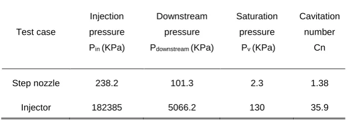
Table II. Operating conditions for the step nozzle and the injector nozzle

simulations. Cavitation number is calculated from equation (11)

Test case

Injection

pressure

Pin (KPa)

Downstream

pressure

Pdownstream (KPa)

Saturation

pressure

Pv (KPa)

Cavitation

number

Cn

Step nozzle 238.2 101.3 2.3 1.38

Injector 182385 5066.2 130 35.9

237

The polymer relaxation times chosen in this study (reported in Table III) are in the range 238

measured for dilute viscoelastic solutions in low viscosity solvents85_{. The molecular}

239

weight of the polymer used in the non-polar solution in the study are reported 6.9 g/mol 240

and 1.6 g/mol for the polymer in the aqueous solution and the concentration range 241

corresponding to the chosen relaxation times is ~ 0.1% wt. The relaxation times are 242

large compared to the flow time scales such as the turnover time of large and small 243

eddies so it is expected that they alter the flow topology. When polymer relaxation 244

times are comparable to flow time scales, the turbulent kinetic energy cascade can be 245

altered resulting in turbulent drag reduction49,86_.

246

To characterize the polymer viscosity, the viscosity ratio βis used (β=

µ

µ

11

viscosities. One of the main objectives of this study is to examine how viscoelasticity 249

can affect the cavitation structures. For this purpose we conducted a preliminary study 250

on the effect of the polymer viscosity and observed clear changes (instantaneous and 251

time-averaged) in cavitation volume fraction when the viscosity of the polymer was 252

large compared to the solvent viscosity. High polymer viscosity values (when β is as 253

small as 0.2)87 _{can damp the turbulent shear stress and contribute to reduction of the}

254

turbulent drag87_.

255

Table III. Fluid properties for the step nozzle and the injector nozzle simulations. *For Diesel liquid viscosity, the Kolev correlation in equation (14) is used, βvalue is then calculated from

the average viscosity in the flow field.

Test case Fluid

Liquid

density ρ_l(Kg/m3₎

Vapor

density ρ_v(Kg/m3₎

Liquid

(solvent)

viscosity µ

s (Pa.s)

Vapor

viscosity µ_v (Pa.s)

Polymer

viscosity µ_p (Pa.s)

Polymer

relaxation

time

λ (s)

Step nozzle

(Newtonian) Water 998.16 1.71E-02 1.02E-03 9.75E-06 - -

Step nozzle

(Viscoelastic) β =0.1 998.16 1.71E-02 1.02E-03 9.75E-06 9E-03 4E-02

Injector

(Newtonian) Diesel 747.65 6.56 Eq 14 7.50E-06 - -

Injector

(Viscoelastic) β=0.1* 747.65 6.56 Eq 14 7.50E-06 2E-02 8E-03

256

257

2.1. Step nozzle test case

258

The geometry of the step nozzle is shown in Figure 1(a) which is based on an 259

experimental study88 _{designed to investigate cavitation in a rectangular injector.}

260

Cavitation development inside the nozzle from incipient condition to fully developed 261

condition is visualized using high speed imaging, moreover laser doppler velocimetry 262

(LDV) measurements of streamwise velocity and RMS of turbulent velocity are 263

12

previously used to examine the performance of the turbulence model and the cavitation 265

model used in the current study 89_{. The data is only available for water and to the best}

266

of author’s knowledge no studies in the literature provide similar data for viscoelastic 267

cavitating flows. 268

Cavitation starts to develop inside the nozzle as water is injected at 0.16 MPa into the 269

atmospheric pressure while the flowrate is 40 mL/s. The injection pressure is increased 270

and cavitation intensifies until fully developed cavitation conditions are reached at 0.31 271

MPa injection pressure and 62 mL/s flowrate. 272

A hemispherical outlet geometry is added to the domain with 14 mm diameter to allow 273

a uniform assignment of the outlet pressure boundary condition away from the nozzle 274

exit and boundary and operating conditions are reported in Table I and Table II. 275

In the simulation test case water flows through the nozzle with a flowrate of 48 mL/s, 276

the pressure difference across the nozzle is 1.38 bar while the injected liquid is 277

discharging into atmospheric pressure. The cavitation number (Cn defined in Equation 278

(11), P_injection, P_downstream and P_v are the injection, downstream and vapor pressures 279

respectively) is 1.38 and the Reynolds number based on average liquid velocity in the 280

nozzle is 27700. These values are similar to those realized in real-size diesel injectors 281

operating at nominal injection pressures and correspond to the incipient cavitation 282

regime 88_:

283

injection downstream

downstream v

P

- P

Cn =

P

- P

(11)

13 285

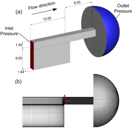
Figure 1. (a) Geometry of the step nozzle and the relevant dimensions in mm, inlet boundary 286

(red color) and outlet boundary (blue color) surfaces are shown all the other surfaces are no– 287

slip walls (grey color) (b)Computational grid with additional refinement inside the nozzle 288

The computational grid consists of unstructured hexahedral cells and additional 289

refinement is used inside the constriction to achieve the cell size below the Taylor 290

length scale λg (approximated from the characteristic length scale L = 1.94 mm and

291

Reynolds number, λg = (10/Re) 0.5 L = 39 µm). Estimation of Taylor microscale provides

292

a guideline for grid resolution in practical LES studies90,91_{; by refining the mesh below}

293

this value the large scale turbulent eddies are captured as λg theoretically lies in the

294

high wavenumber end of the inertial subrange. Taylor length scale characterizes the 295

mean spatial extension of the velocity gradients92,93 _{and is always much smaller than}

296

the integral scale (but not the smallest scale)94. The cell size inside the nozzle is 20 µm

297

and it is refined to 2.5 µm near the walls, corresponding to y+ _{values of 0.2-1. The time}

298

step corresponding to Courant-Friedrichs-Lewy (CFL) number of 0.5 is set to 1 µs in 299

the Newtonian test case and for the viscoelastic case the time step is reduced to 0.5 µs 300

14

2.2. Injector nozzle test case

302

A common rail injector geometry section as shown in Figure 2 is simulated which has a 303

more complex flow and cavitation mechanism compared to the step nozzle. This is a 304

real-size Diesel fuel injector tip with five uniformly distributed holes and the nozzle 305

holes are slightly tapered with a

k

in out

D - D

k =

10

(12)

307

D

D

308

nozzle has an inlet and exit diameter of 0.37 mm 0.359 mm respectively and is 1.26 309

mm long. Nozzle hole tapering is linked to reduction of cloud cavitation but at the same 310

time, formation of vortex or string cavities (presented in results section in Figure 10) 311

inside the nozzle. By using taperd holes instead of cylindrical holes, string cavitation 312

which forms inside large scale vortices entering the nozzle from the sac volume, can be 313

intensified while cloud cavitation is reduced 70_{. In this test case, the fuel passes through}

314

the needle passage before entering the sac volume (see Figure 2), where it recirculates 315

as it enters the nozzle. A cavitation cloud forms at the top corner of the nozzle entrance 316

due to the sharp turn in the flow streamline. Moreover, a large vortex enters the nozzle 317

from the sac volume, with string cavitation forming in the core of this vortex inside the 318

nozzle. A recent fully compressible implicit LES simulation of a 9-hole injector with 319

needle motion95 _{shows that elongated vortical structures which enter the nozzle from}

320

the sac volume and the overall flow features are present when compared to steady 321

needle simulations at full needle lift. 322

The Reynolds number inside the nozzle and the sac volume reaches above 30,000 323

indicating the highly turbulent flow conditions of the injector. Considering the mesh 324

15

cost of simulating the complete 5 hole geometry for Newtonian and viscoelastic fluids 326

would be very high so 1/5th _{of the injector geometry (72}˚_{) is simulated as shown in}

327

Figure 2 (b) and periodic boundary conditions are employed on the sides of the 328

geometry. 329

330

Figure 2. (a) Simulation domain for the injector test case. Boundary condition are indicated by 331

colored surfaces; inlet and outlet boundaries are colored in red and blue respectively and the 332

green surface shows the periodic boundary (another periodic boundary with the same cross 333

section is located on the opposite side of the geometry), all the other surfaces are no–slip walls 334

(grey color), (b) The computational grid for the injector, the domain is partitioned using blocking 335

and it is hex-dominant except from an unstructured tetrahedral section in the sac volume 336

Inlet and outlet total pressures are fixed at Pinjection = 1800 bar and Pdownstreamt = 50 bar.

337

Cavitation number for this condition is Cn =35.9, which is much higher than the step 338

nozzle test case due to the higher pressure difference from the inlet to the outlet. In this 339

condition fully developed cloud cavitation is located in the top surface of the nozzle, 340

while the string cavity has a more intermittent appearance. 341

A hex-dominant block mesh is used for most parts of the geometry, except for a section 342

in the sac volume upstream of the nozzle entrance, where unstructured tetrahedral 343

mesh is used. The mesh resolution in the nozzle and the sac volume where cavitation 344

develops is 7.5 µm with additional refinement near the walls. With this resolution, large 345

16

captured. The time step for the Newtonian flow condition is 5 ns for CFL of ~0.4 and for 347

the viscoelastic case it is reduced to 2 ns and CFL of ~0.15. 348

The pressure levels inside the injector change significantly so the subsequent changes 349

in the Diesel fuel properties are also considered. Hence the density and the viscosity of 350

the fuel are calculated as a function of pressure. The density is calculated using Tait 351

equation of state to represent the weak compressibility of the liquid Diesel: 352

n

sat sat,L

p B

ρ

ρ

_{ } 

 

= _ _ − +

_{ } 

 

(13)

353

where the bulk modulus

B

sat

P are the liquid saturation density and saturation pressure respectively. The liquid 355

viscosity is calculated based on the correlation proposed by Kolev96 _:

356

6 L

10 5

10 0.000234373 p

log 0.035065275 -

10

µ ρ

 

=

 

 

 

(14)

357

The values used for the fluid properties used in both test cases can be found in Table 358

III. 359

3. Results and discussion

360

3.1. Step nozzle

361

As the flow detaches at the entrance of the nozzle (see Figure 3) a shear layer is 362

formed between the flow passing through the nozzle and the recirculation region. 363

Cavitation vapors appear in the core of microvortices in the shear layer and they are 364

detaching and shedding from the cavity cloud in a cyclic manner. Contours of velocity 365

magnitude in the mid-plane of the nozzle for the Newtonian and the viscoelastic fluids 366

17

to have a more homogenous gradient. The black iso-lines show the areas where the 368

pressure drops below the vapor pressure, i.e. the regions of cavitation inception. The 369

cavitation inception regions appear more frequently in the Newtonian fluid and they 370

cover a larger area of the nozzle’s cross sectional area, indicating that more vapor is 371

being produced in this fluid. It is likewise reported in the literature that the minimum 372

pressure at a cavitation inception point (the core of a vortex developing in the wake of a 373

cylinder) increases as the vorticity is reduced by viscoelasticity 97_.

374

375

Figure 3. Nozzle geometry and cavitation in the shear layer (top), contours of the velocity 376

magnitude for the Newtonian and the viscoelastic fluid in the mid-plane of the nozzle, the black 377

iso-lines show regions with pressures below the vapor pressure (bottom) 378

The structure of the vortical features in the flow is shown in Figure 4 by means of the 379

second invariant of the velocity gradient tensor98 _{calculated from i} j A

1 II

2 ∂ ∂ = −

∂xj ∂xi

u u

. 380

Spanwise Kelvin-Helmholtz-like vortices form right after the nozzle inlet as shown in 381

Figure 4 (a), it can be clearly seen that significantly fewer vortices appear in the 382

viscoelastic fluid. Inhibition of shear instability by polymer injection has previously been 383

reported in the literature 99_{. The ‘polymer torque’, which is the contribution of the}

384

viscoelastic stress to the vorticity evolution, increases the flow resistance to rotational 385

motion and can inhibit the vortex sheet roll-up97_.

18

Further downstream, the vortex sheet breaks down, developing a range of small-scale 387

and large-scale structures. It is evident that in the viscoelastic fluid spanwise vortices 388

are inhibited while longitudinal vortices become more dominant. Enhancement of large 389

scale coherent structures in the mixing layer is due to hindering of development of 390

perturbations and a stronger vorticity diffusion in viscoelastic fluids100_{. This results in}

391

slower rotational motion of the neighboring vortices and delay of vortex pairing and 392

merging, therefore the lifetime and the scale of the coherent structures is increased. 393

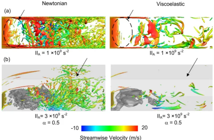
394

Figure 4. (a) Iso-surface of the second invariant of the velocity gradient with the value 1×109 _s-2

395

colored with the streamwise velocity, image shown from the top (–Y) direction (b) 3D view of the 396

iso-surface of the second invariant of the velocity gradient at 3×109 _s-2 _{colored with the}

397

streamwise velocity along with iso-surface of 50% vapor volume fraction (grey color) 398

In Figure 4 (b) the iso-surface of 50% vapor volume fraction is presented along with the 399

IIA iso-surface. After the collapse of the cavity cloud in the Newtonian fluid, a strong

400

mixing region forms inside the nozzle. In the viscoelastic fluid however, the mixing is 401

weaker and mainly vortices with larger diameters are forming as local instabilities are 402

suppressed and vortical sub-structures are damped. Likewise enlargement of 403

19

reported in turbulent channel flows 101_{. This is due to tendency of polymers to strongly}

405

align in the streamwise direction, partially suppressing wall-normal and spanwise 406

velocity fluctuations102_{. Moreover, the polymer viscosity resists the extensional}

407

deformation imposed by the motion of turbulent eddies103,104_.

408

The turbulence kinetic energy spectrum for the Newtonian and the viscoelastic fluid is 409

shown in Figure 5, where k is the wave number and E(k) is the amplitude of the kinetic 410

energy FFT calculated inside the nozzle. The graph represents the spatial spectrum of 411

the turbulence kinetic energy, where k = 2πn/L and n and L are the incremental spatial

412

frequency number and the wavelength respectively. 413

Energy content of the low wavenumber scales is higher by ~15% in the Newtonian 414

fluid, however the decay slope is also slightly faster (-5/3 in the Newtonian fluid in 415

competition with ~-4/3 in the viscoelastic fluid) so the flow energy mainly contained 416

within the inertial subrange eddies is similar in both cases. 417

At higher wavenumbers the difference becomes more evident as the Newtonian fluid 418

has ~38% higher turbulence kinetic energy content, indicating that the small-scales in 419

this fluid are more pronounced. This observation is expected as the small-scales are 420

suppressed in the viscoelastic fluid as seen in Figure 4. This is consistent with 421

experimental measurements of power spectra in wall-bounded polymeric flows which 422

show that viscoelasticity can suppress turbulence kinetic energy at small-scales while 423

having a negligible effect on large scales105_{. Moreover, in viscoelastic fluids, the kinetic}

424

energy removed from the large scales is partially dissipated by small-scales and 425

partially converted into elastic energy which is then transferred back into the large 426

scales. This will alter the nature of energy cascade usually seen in Newtonian fluids 427

and reduce the energy content at the small-scales106_.

20 429

Figure 5. Energy spectra inside the step nozzle for the Newtonian and the viscoelastic fluid, 430

dashed lines (- - - - - and - - - - -) show indicative examples of the spectra and continuous lines (



and



In Figure 6 (a) the development of the streamwise velocity component in the mid-plane 433

of the nozzle presented. The magnitude of the negative velocity in the recirculation 434

region (-0.94 ≤ Y ≤ -0.4) is larger in the Newtonian fluid on average by ~28% at X = 435

2mm and ~41% at X = 4 mm. The re-entrant jet velocity is responsible for detachment 436

and shedding of the cavity cloud 71_{, therefore larger velocities in the recirculation region}

437

of the Newtonian fluid are indicative of a faster shedding process in this fluid. 438

In Figure 6 (b), the RMS of streamwise velocity which indicates the turbulent velocity, is 439

plotted along the nozzle. Overall the weighted average of RMS of streamwise velocity 440

over the computational cell volume inside the nozzle (0 mm < X< 8 mm) is reduced by 441

11% in the viscoelastic fluid. In Figure 6 (b), this effect is mainly visible in the lower half 442

of the nozzle (-0.94 mm ≤ Y ≤ 0 mm), corresponding to the shear layer and flow 443

recirculation regions. Theeffect of viscoelasticity on velocity fluctuations is more 444

evident in Figure 6 (c) which shows the RMS of wall-normal velocity along the nozzle. 445

Suppression of velocity fluctuations is stronger in the wall-normal direction compared to 446

the streamwise direction and overall the RMS of wall-normal velocity is reduced by 447

21

velocity fluctuations, polymers can more effectively reduce the turbulence generation 449

by vortices. 450

451

Figure 6.Comparison of time-averaged values of the streamwise velocity, RMS of streamwise 452

velocity, RMS of wall-normal velocity and Reynolds stress (−u v′ ′) in the Newtonian and the 453

viscoelastic fluid, data are presented in the mid-plane of the step nozzle at four different X 454

22

In Figure 6 (d) the Reynolds stress in the XY plane (

−

u

′

v

′

positive and negative values of the Reynolds stress correspond to turbulence 457

suppression and production respectively107_{. Negative values of Reynolds stress are}

458

produced by ejection and sweep motions which contribute to positive turbulence 459

production and in general increase drag. Positive Reynolds stress values correspond to 460

turbulence suppression and their increase generally results in drag reduction 107_{. It is}

461

evident that in the recirculation region (-0.94 mm ≤ Y ≤ 0 mm) the Newtonian fluid has 462

about twice the amount of Reynolds stress generated in the viscoelastic fluid, resulting 463

in a higher level of turbulence generated in this region. In the bulk of the flow outside 464

the recirculation zone, Reynold stresses have a positive value with a higher magnitude 465

in the viscoelastic fluid indicating a stronger turbulence damping. Overall, stronger 466

turbulence damping and lower turbulence levels generated in the viscoelastic fluid as 467

seen in Figure 6 (b)-(d), can contribute to turbulence drag reduction and the mass 468

flowrate is increased by~2%. 469

In Figure 7 the development of cavitation inside the nozzle for the Newtonian and the 470

viscoelastic fluid is compared in terms of 25% vapor volume fraction iso-surface. 471

Cavitation is initiated in the core of microvortices forming in the shear layer and it grows 472

as larger eddies form after the vortex sheet breakdown. Following, they form a cavity 473

cloud which detaches due to the re-entrant jet motion and is convected toward the 474

nozzle exit. 475

In the Newtonian fluid, small cavitation structures can be observed (red circle 1) with 476

microcavities of various sizes (approximate diameter range of 30 µm-200 µm) shedding 477

from the cloud, however such structures are not present in the viscoelastic fluid. 478

23 480

Figure 7.Cavitation development inside the step nozzle presented by means of 25% vapor 481

volume fraction iso-surfaces, data are presented every 0.1 ms. Small microcavities shedding 482

from the cloud (red circle 1) are not present in the viscoelastic fluid, cavitation vapors can 483

initially shrink before growing (red circle 2) and larger streamwise vortices appear between the 484

detached cloud and shear layer cavitation structures (red circle 3, 4 and 5) 485

The growth of the shear layer cavitating microvortices is rather faster in the Newtonian 486

fluid; in the viscoelastic fluid it appears that the cavity initially shrinks (red circle 2) 487

before growing. This can be due to the action of viscoelastic force resisting the fast 488

deformation by liquid evaporation. Furthermore, cavitation structures in the viscoelastic 489

fluid have an elongated shape. Larger streamwise cavitating vortices appear between 490

the shear layer cavities and the detached cloud compared to the Newtonian fluid (see 491

red circles 3, 4 and 5). 492

Due to the cyclic enlargement and shrinkage of the flow recirculation zone and the 493

24

nozzle also fluctuates in a cyclic manner. The fast Fourier transform (FFT) of mass flow 495

rate time-evolution at nozzle outlet are presented in Figure 8 to indicate the dominant 496

frequencies of the mass flowrate fluctuations. The dominant frequency in the 497

Newtonian fluid is f = 168 Hz whereas in the viscoelastic fluid this values is reduced to f 498

= 57 Hz, while the peak amplitude is increased by 42%. First and second harmonics of 499

the dominant frequency can also be identified for both fluids at ~ 2f (343 Hz for the 500

Newtonian fluid and 110 Hz for the viscoelastic fluid) and ~3f (524 Hz for the 501

Newtonian fluid and 169 Hz for the viscoelastic fluid). Second harmonics with about 502

double the dominant frequency are reported in pressure signals past a cavitating 503

converging-diverging nozzle108 _{and in the wake of a rectangular cavitating obstacle}109_.

504

The reduction of the cavity shedding frequency can be due to the resistance of the 505

viscoelastic fluid to development of vortical structures and therefore suppression of 506

cavity growth in the core of vortices. Moreover, development of the cavitation cloud can 507

be delayed as the cavity volume can shrink before growing in the viscoelastic fluid due 508

to memory effects produced by fluid elasticity. In fact it was observed that some of the 509

shedding events are completely suppressed while vapor builds-up in the cloud region. 510

Therefore the subsequent shedding event is more violent in the viscoelastic fluid, thus 511

while the dominant frequency is reduced its peak amplitude is higher. 512

Unlike the Newtonian fluid, at frequencies above ~400Hz there are effectively no 513

fluctuations in the viscoelastic fluid, indicating that the viscoelastic fluid damps out the 514

high frequency fluctuations. As the small-scale microcavities shedding from the 515

cavitation cloud are suppressed (Figure 7), the subsequent velocity fluctuations due to 516

growth, collapse and oscillations of these cavities can also be inhibited, resulting in 517

25 519

Figure 8. FFT of mass flowrate fluctuations at the outlet of the step nozzle for the Newtonian 520

and the viscoelastic fluid, the dominant frequency corresponds to frequency of mass flowrate 521

fluctuations induced by cyclic growth and shedding of large cavity clouds 522

The Strouhal number for vapor cloud shedding (St ) based on the mass flowrate _v 523

fluctuation frequency (f), the cavity length (L ) and the average streamwise velocity in _v 524

the cavity region (U ) is defined as: _v 525

v v

v

fL

St =

U

(15)

526

For the Newtonian case the Strouhal number based on the dominant frequency is 0.22 527

and in the viscoelastic fluid the Strouhal number is reduced to 0.08. For Newtonian 528

fluids, a characteristic Strouhal number of 0.2 has been identified for cavitation cloud 529

shedding in a diverging step71_{. The detachment and shedding of the cavitation cloud is}

530

partially driven by the re-entrant jet mechanism and the Strouhal number is 531

proportional to the re-entrant jet velocity 71_{, hence longer shedding periods can be due}

532

to reduction of the re-entrant jet velocity. Observations regarding the reduction of 533

Strouhal number by viscoelasticity due to prolonged oscillation times has been reported 534

for vortex shedding past an obstacle 110–112_.

26 536

Figure 9. (a) Average liquid volume fraction (1-α) in the step nozzle mid-plane along with iso-537

surfaces of 75%, 80% and 85% average liquid volume fraction in the Newtonian and the 538

viscoelastic fluid, (b) Average liquid volume fraction (1-α) inside the cavitation region for the 539

Newtonian and the viscoelastic fluid, values taken along 4 lines passing through the cavitation 540

cloud in the nozzle mid-plane 541

Finally, the time-averaged effect of viscoelasticity on the cavitation field is presented in 542

Figure 9 by comparing the average liquid volume fraction inside the nozzle. It can be 543

seen from Figure 9 (a) that the cavitation inception point is shifted further downstream 544

the nozzle entrance; so vapor mainly starts to form at X ≈ 0.3 mm in the Newtonian 545

fluid and at X ≈ 0.8 mm in the viscoelastic fluid. Moreover the thickness of the cavity

546

cloud in this region is reduced from ~0.69 mm in the Newtonian fluid to ~0.58 mm in 547

27

In Figure 9 (b) values of the liquid volume fraction in four locations inside the cavitation 549

cloud are compared. In all these locations the liquid volume fraction in the viscoelastic 550

fluid is constantly higher. The average vapor volume fraction in the viscoelastic fluid 551

integrated over the volume of the nozzle (0 mm < X < 8 mm) is reduced by 51%. 552

Moreover it is evident that the cavitation suppression effect is stronger at the lower half 553

of the cavity cloud -0.94 mm ≤ Y ≤ -0.5 mm (closer to the nozzle wall). Reduction of 554

near wall vorticity fluctuations inhibits the near-wall eddies in viscoelastic fluids113 _which

555

can be responsible for production and transport of cavitation vapors in this region. 556

557

3.2. Injector nozzle

558

In the injector nozzle, two distinct regions for cloud cavitation and string cavitation can 559

be identified. Characteristics of different cavitation mechanisms in injector nozzles is 560

described in the literature 70,114,115_{. The cloud cavitation forms in a similar manner to the}

561

cavitation in the step nozzle; as the fluid enters the nozzle it takes a sharp turn at the 562

entrance forming a fully developed vapor cloud which is mainly attached to the top 563

surface of the nozzle and grows and sheds in a cyclic manner. The string cavitation 564

forms in the high vorticity core of a large vortex entering the nozzle from the sac 565

volume and it is located in the vicinity of the nozzle center (the streamlines and vectors 566

forming the string cavitation are presented in Figure 10 (a)). 567

The local pressure drops from 100 MPa in the sac volume to 0.1 MPa (below the 568

saturation pressure) inside the nozzle as the string cavity starts to form. The string 569

cavity has an intermittent appearance as it can distort, break-up and elongate inside 570

the nozzle, however in the viscoelastic fluid a larger and more stable vaporous core 571

appears and time averaged values of vapor volume fraction will be used to further 572

28 574

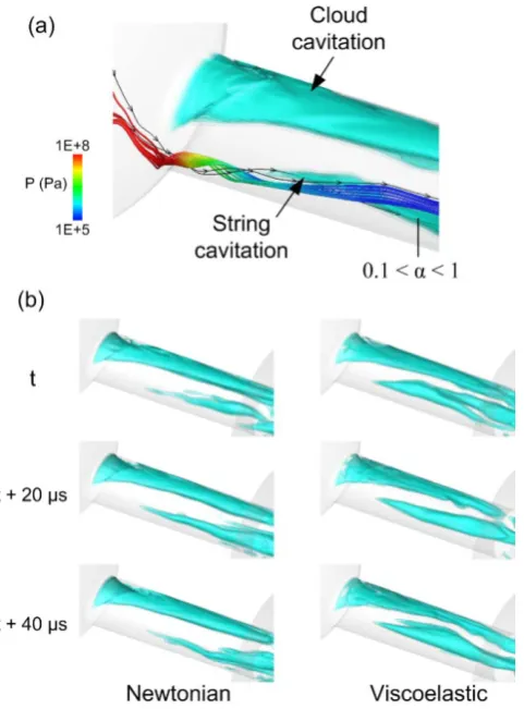
575

Figure 10. (a) Two distinct cavitation regions forming inside the injector nozzle, cavitation 576

vapors are presented using 5 translucent vapor volume fraction iso-surfaces ranging from 0.1 to 577

1, the cavitating vortex can be seen entering the nozzle from the sac volume, the vortex is 578

presented by streamlines colored with pressure (b) Indicative cavitation structures inside the 579

nozzle at 20 µs intervals for the Newtonian and the viscoelastic fluid (0.1< α <1) showing a 580

larger string cavity in the viscoelastic fluid. 581

Since the cloud cavitation and the string cavitation occur at different locations inside 582

the nozzle, it is possible to examine the effect of viscoelasticity on each cavitation 583

mechanism by geometrically separating the cavitation vapor volumes as seen in Figure 584

11 (a), which shows the separated cloud and the string cavitation structures in the 585

same time step. The time-averaged vapor volume fraction data are separated into a 586

cloud region and a string region by splitting the cross section of the nozzle into a top 587

section (cloud, Y>35 µm) and a bottom section (string, Y<35 µm) using a plane along 588

29

calculated in slices along the nozzle and the area weighted average value is used to 590

get the total vapor volume fraction. Vapor structures in the cloud and the string region 591

marginally intersect inside the nozzle but in the vicinity of the nozzle exit this overlap 592

can contribute to ~20% variations in the average vapor volume fraction in each region. 593

The overlapping regions are identified to be located in the area approximately ±40µm 594

from the nozzle axis and are displayed in the graph as error bars. 595

The time-averaged value of the total vapor volume fraction inside the nozzle is plotted 596

for the Newtonian and the viscoelastic fluid in Figure 11 (b). It is evident that the in-597

nozzle cavitation mechanism is mainly due to cloud cavitation in the Newtonian fluid 598

and overall the vapor volume fraction in the Newtonian fluid is higher by 44%. Initially, 599

cavitation develops at the nozzle entrance due to the cloud cavitation mechanism, 600

increasing the vapor volume fraction in the nozzle up to ~0.16 in the Newtonian fluid 601

and up to ~0.08 in the viscoelastic fluid until X ≈ 0.4 mm. After this point cloud

602

cavitation declines and string cavitation starts to develop while reaching the nozzle exit. 603

In the viscoelastic fluid the vapor volume fraction of the cloud cavitation is higher than 604

string cavitation up to X ≈ 0.9 mm (70% into the nozzle length), and after this location 605

the string cavitation becomes more dominant. In the Newtonian fluid the rate of 606

reduction of the cloud cavity is ~17% faster than the rate of formation of string cavity, 607

hence the total vapor volume fraction is reduced after X ≈ 0.4 mm. Whereas in the 608

viscoelastic fluid, the string cavitation forms more abruptly at a rate ~46% faster than 609

the decline of the cloud cavity, hence the total vapor volume fraction increases steadily 610

up to X ≈ 1 mm, after this point vapor volume fraction is reduced as string cavitation

611

growth declines. 612

The main observation from comparing the changes in the vapor volume fraction in 613

different mechanisms is that viscoelasticity reduces cavitation formation in the cloud 614

30

of the cavitating vortex in the nozzle core is increased in the viscoelastic fluid which 616

can be related to the alignment of the cavitating vortex with respect to the main flow 617

direction. The string cavitation is forming in the core of the quasi-streamwise vortex in 618

the center of the nozzle, whereas the cloud cavitation vortices can have large radial 619

velocity components which are expected to be inhibited by viscoelasticity. 620

In the core of vortices the angle between the velocity vector (U) and the vorticity vector 621

(ω) tends to zero as the vectors become aligned, hence the normalized helicity (Hn),

622

which is effectively the cosine of this angle, tends towards unity 116_:

623

n U. H

U

ω ω

=

(16)

624

The normalized helicity contours are plotted in Figure 11(c) in several locations inside 625

the nozzle along with black isolines of Hn = 0.95. It is evident that in the viscoelastic

626

fluid, the string cavitation core covers a larger area, whereas in the Newtonian fluid a 627

smaller vortex core can be identified. In the step nozzle test case presented in the 628

previous section, it is reported that the streamwise vortices become more dominant by 629

viscoelasticity as the smaller scale vortices are damped. In wall-bounded viscoelastic 630

flows117,118 _{it is reported that streamwise vortices can become elongated and larger as}

631

wall-normal fluctuations are damped. It is argued that suppression of cross-stream 632

fluctuations can further inhibit their auto-generation and therefore increase the lifetime 633

and strength of the longitudinal vortices. Likewise in this case, suppression of small-634

scale eddies inside the injector nozzle can be responsible for stabilizing the local 635

turbulence in the vicinity of the string cavity, allowing the development of a larger 636

streamwise vortex and delaying the vortex breakdown, which in turn can result in 637

31 639

Figure 11. (a) Separated vapor volume fraction regions inside the injector nozzle showing the 640

cloud cavitation and the string cavitation in term of iso-surfaces of 80% vapor volume fraction, 641

(b) Development of the string cavitation (dotted lines• • • • • • and • • • • • •), the cloud cavitation (dashed

642

lines













injector nozzle for the Newtonian and the viscoelastic fluid calculated in slices along the nozzle 644

axis using area weighted averages, error bars indicate the overlap of the vapor volume fraction 645

in the string and cloud the region in ±40µm in the vicinity of the nozzle axis,(c) Normalized 646

helicity (Hn) contours in slices inside the injector nozzle (at X = 0.2 mm, 0.5 mm, 0.8 mm and 1.1

647

mm), the black isolines show the regions of Hn = 0.95 and Hn→1 in vortex cores

648

In the cavitation model of Schnerr and Sauer 78 _{in equation (7), the vapor volume}

649

fraction equation source term describes the mass transfer rate (R) between the two 650

phases, so the positive values of R represent the evaporation rate and the negative 651

values are the condensation rate: 652

V v l

V

m B l

p p

3 2

R (1 ) (p p)

3

α α  − 

= − −

 

ℜ  

ρ ρ

sign

ρ ρ (17)

653

In Figure 12 (a) and (b) the phase change rates in the cloud cavitation and the string 654

cavitation region at one instance are compared. The mass transfer rates are higher in 655

the cloud cavitation region, reaching 15 × 106 _Kg/m3.s as opposed to 0.5 × 106 _Kg/m3_.s

32

in the string region of the Newtonian fluid, subsequently cloud cavitation is the main 657

mechanism of vapor production as it was seen in Figure 11 (b). In the cloud cavitation 658

graph, mass transfer starts at the X = 0 mm as the fluid enters the nozzle and peaks at 659

X ≈ 0.25 mm, however the string cavitation starts effectively at X > 0.2 mm in the

660

viscoelastic fluid and X >0.4 mm in the Newtonian fluid. The evaporation and 661

condensation rates in the cloud region are reduced in the viscoelastic fluid by ~2 orders 662

of magnitude, resulting in reduction of the vapor volume fraction in this region. However 663

in the string cavitation region this trend is reversed, i.e. evaporation rate is ~9 times 664

higher and condensation rate is ~2.5 times higher in the viscoelastic fluid. 665

The difference in the effect of viscoelasticity on cloud and string cavitation regimes can 666

be linked to the alignment of the vortical structures in each region with respect to the 667

direction of the main flow. The vortex cores identified in terms of the second invariant of 668

the velocity gradient are presented in Figure 12 (c). It is evident that viscoelasticity 669

does not affect the cloud and string vortical structures in the same manner. The vortex 670

which forms the string cavitation in the vicinity of the nozzle center (see arrow 1), is 671

enlarged by viscoelasticity while the vortical structures formed at the nozzle entrance in 672

the cloud region (see arrow 2) are strongly suppressed and only remnants of the 673

vortices are visible in the viscoelastic fluid. In the cloud cavitation region, vortices form 674

in the shear layer between the recirculating flow and the main flow, therefore they can 675

have large radial velocity components as the vorticity vector is likely to be located in the 676

cross-sectional plane of the nozzle (i.e. vortices rotating out of the cross sectional 677

plane). However in the string region the cavitating vortex is positioned in the 678

streamwise direction (vorticity vector in the axial direction). Therefore, as the polymers 679

tend to align with the main flow direction102 _{and suppress the cross flow fluctuations}87_,

680

viscoelasticity tends to damp the vortices in the cloud region while stimulating the string 681

33 683

Figure 12. (a) and (b) evaporation and condensations rates computed by the mass transfer rate 684

cavitation model in the cloud and the string cavitation region, (c) vortical flow structures in the 685

vicinity of the injector nozzle entrance plotted using the contours of second invariant of the 686

velocity gradient (Q-criterion) in the nozzle mid-plane and translucent iso-surfaces of Q-criterion 687

at 5E+12 s-2

688

As it was mentioned earlier, the vortex forming the string cavitation enters the nozzle 689

from the sac volume and is formed by the swirling flow inside the sac volume 70_{. Hence}

690

the level of turbulence upstream the nozzle entrance, can have a significant effect on 691

the strength of the cavitating vortex. In Figure 13 (a) the flow structures in the sac 692

volume in terms of the second invariant of the velocity gradient are displayed. 693

Circumferential perturbations on the interface of a cavitating vortex can cause strong 694

radial oscillations which result in splitting and collapse of the cavity core119_{. Moreover,}

695

flow instabilities upstream the vortex can cause the divergence of the stream tubes 696

forming the vortex core, eventually breaking down the vortex 120_{. The turbulent eddies}

697

in the sac volume in the Newtonian fluid (Figure 13 (a)) appear to breakdown the 698

34

or delay the vortex breakdown as it prevents sharp velocity variations along the vortex 700

centerline which initiate the breakdown process 121_.

701

702

Figure 13. (a) Vortex structures indie the sac volume visualized using the iso-surface of second invariant of 703

the velocity gradient at 4E+12 s-2_{, (b) velocity fluctuations inside the nozzle plotted in terms of RMS of X,Y}

704

and Z velocity, values obtained from surface-averaged data calculated in slices along the nozzle 705

The vortex disturbance inside the sac volume is significantly lower in the viscoelastic 706

fluid compared to the Newtonian fluid in Figure 13 (a) and the large vortex entering the 707

nozzle can be clearly identified. Reduction of vortex interactions in the sac volume 708

contributes to stabilization of the cavitating vortex upstream of the nozzle entrance, 709

which in turn allows a stronger string cavity to develop inside the nozzle. The 710

fluctuations inside the nozzle in terms of RMS of the velocity components are plotted in 711

Figure 13 (b). It is evident that due to the stabilizing effect of viscoelasticity on flow 712

turbulence, all three components of velocity fluctuations are reduced in the viscoelastic 713

fluid (by 23%, 9% and 31% in X, Y and Z directions respectively). This will therefore 714

reduce the perturbations that destabilize the string cavity coherence inside the nozzle, 715

allowing the cavitation structures to last longer. 716