The drag force in two-fluid models of gas-solid flows

Shorter Communication

The drag force in two-fluid models of gas-solid flows

Yonghao Zhang

a

and Jason M. Reese

b

a

Department of Computational Science and Engineering, Daresbury Laboratory, Daresbury, Warrington, WA4 4AD, UK

b _{Department of Mechanical Engineering, King’s College London, London WC2R 2LS, UK}

1. Introduction

Currently, the two most widespread methods for modelling the particulate phase in numerical simulations of gas-solid flows are discrete particle simulation (see, e.g., Mikami, Kamiya and Horio 1998), and the two-fluid approach, e.g. kinetic theory models (see, e.g., Louge, Mastorakos and Jenkins 1991). In both approaches the gas phase is described by a locally-averaged Navier-Stokes equation and the two phases are usually coupled by a drag force. Due to the large density difference between the particles and the gas, inter-phase forces other than the drag force are usually neglected, so it plays a significant role in characterising the gas-solid flow. Yasuna, Moyer, Elliott and Sinclair (1995) have shown that the solution of their model is sensitive to the drag coefficient. In general, the performance of most current models depends critically on the accuracy of the drag force formulation.

2. Problems with the drag force formulation

The drag force experienced by a spherical particle of diameter d moving in an infinite fluid of density 1 is given by

(

V u

)

u

V − −

= 2 ₁

8C d

f_drag π _D , (1)

where u is the velocity of the particle, V is the fluid velocity at infinity, and CD is the drag

coefficient. If the particle is surrounded by many others, and the local particle volume fraction is ε2, the drag force volume-averaged over a cell containing only a single particle should be given by

(

V u

)

v u

(

v u

)

f = − = − −

d C_D drag

1 2 4

3 ε ρ

β , (2)

this fluid over δV1. However, the particle volume fraction has been proven to have a more complex and subtle influence on the drag force (e.g. Wen and Yu 1966; Di Felice 1994). Generally, the momentum transfer coefficient, β, can be expressed as

(

2 1

2 4

3 ε ρ _ε

β f

d

C_D v −u

=

)

, (3)

and many forms for the correction factor f(ε2) have been proposed. For example, Di Felice (1994) gave

( )

_{ε =ε} −χ 2 2

f , (4)

where χis an empirical coefficient, which depends on the particle Reynolds number Repvia

(

_⎥⎦⎤ ⎢⎣ ⎡_{− −} − = 2 10Re log 5 . 1 2 1 exp 65 . 0 7 . 3 _p

χ

)

. (5)

In discrete particle simulations, the usual expressions for the momentum transfer coefficient are extended from the work of Ergun and Orning (1949), Ergun (1952) and Wen and Yu (1966), where the influence of solid volume fraction is incorporated:

8 . 0 , 75 . 1

150 ₂ 2 1 ₁

1 2

2 + − <

= ε ρ ε

ε μ ε

β v u

d

d , (6)

8 . 0 , 4 3 1 65 . 2 1 1

2 − ≥

= ε ρ _ε − _ε

β v u

d

C_D , (7)

where is the fluid viscosity and ε1 is the local fluid volume fraction such that ε1+ε2=1. Despite the inconsistency at ε1=0.8 for equations (6) and (7), numerical simulations using these formulations show good agreement with experimental data from pneumatic conveyors and fluidised beds (Kawaguchi, Tanaka and Tsuji 1998; Mikami, Kamiya and Horio 1998; Hoomans, Huipers, Briels and van Swaaij 1996).

However, the work of Ergun and Wen and Yu has also been widely adopted within many two-fluid models for gas-solid flows, where the particulate and fluid velocities are averaged over the much larger volume δV2 which contains statistically many particles (see Figure 1). For example, Neri and Gidaspow (2000) and Nieuwland, van Sint Annaland, Kuipers and van Swaaij (1996) use momentum transfer coefficients of a similar form to those given in equations (6) and (7) above, viz.

8 . 0 , 75 . 1

150 2 1 ₁

2 1

2 2

1 = + − ε <

ρ ε ε

μ ε

β V U

d

8 . 0 ,

4 3

1 65

. 2 1 1

2

1 = − ≥

− _ε

ε ρ

ε

β V U

d

C_D . (9)

where V and U are the gas and particle velocities, respectively, averaged over the element volume δV2. If we assume that, at least, V equals v for the gas, the only difference between equation pairs (6) and (8), and (7) and (9) is whether an instantaneous or an averaged particulate velocity is used.

The original phenomenological Ergun formula is based on observations on a fixed bed where the particles have no relative motion. If it is to be extended to freely moving particles, not only the particle volume fraction but also the random fluctuational velocity of individual particles should be considered. The work of Wen and Yu also only addressed the effect of voidage on the drag force. If we assume the drag force acting on a particle surrounded by others can be expressed by equations (2) and (3), the averaged drag force in a two-fluid model can be re-derived as follows.

3. A new expression for the averaged drag force

Anderson and Jackson’s (1967) rigorously-derived two-fluid model for particle-fluid flows required volume-averaging the point equations of motion for the fluid and individual particles. In order to smooth out high frequency fluctuations, the elemental volume chosen for this was δV2, rather than δV1 (see Figure 1). The choice of the requisite volume element is discussed in Anderson and Jackson (1967).

( )

_⎥ ⎦ ⎤ ⎢ ⎣ ⎡ ′ − = ′ T T f 2 exp ) 2 ( 1 2 2 3 ) 0

( _u u

π , (10)

where T is the granular temperature, given by 1/3 u′2 .

The averaged drag force over δV2, containing n particles, i.e. n cells each of volume δV1, can be given by

) ( ) ( 1 u u f f

F =

∑

=

∫

′ ′

∞ ∞ − = d f drag n i i drag,

drag , (11)

where f(u′) is particle velocity distribution function. Substituting equations (2) and (3) into this equation, and assuming the gradient of the fluid volume fraction is negligible in the elemental volume δV2, we obtain

(

)

( ) ( ) ) ( 4 3 2 1

2 _{V U u V U u u u}

F =

∫

− − ′ − − ′ ′ ′

∞ ∞ − d f f d C_D drag ε ρ ε

, (12) where the drag coefficient, CD, is treated as an “averaged value” over δV2. Under the assumed Maxwellian distribution of the particle fluctuation velocity, we find

π

T d

f (0)( ′) ′= 8

′

∫

∞ ∞ − u u

u . (13)

If 8T/π < U−V , which is satisfied by most gas-solid flows in pneumatic conveying systems and circulating fluidised beds, equation (12) then becomes

(

)

( ) ( ) ( )

4

3 (0)

2 1

2 _{V U V U u u u}

F ≈ −

∫

− − ′ ′ ′

∞ ∞ − d f f d C_D drag ε ρ ε

, (14) If F_drag is expressed in the standard form β₀(V −U), then,

( )

( ) ( )

4

3 (0)

2 1 2

0 =

∫

V −U −u′ u′ u′

∞ ∞ − d f f d

C_Dε ρ ε

β

(

)

( )

₂

2 1 2 1 2 8 4 3 _ε π ρ ε f T d

C_{D ⎢⎣}⎡ − + _⎥⎦⎤

≈ V U

2 1

( )

₂

4

3 ε ρ _ε

f U d

C_{D r}

= . (15)

Here, U_r is defined as the mean magnitude of the slip velocity:

(

)

2 8 12

⎥⎦ ⎤ ⎢⎣ ⎡ _{− +} = π T

Because there are many different formulas for the standard CD, and further uncertainty is

inevitably introduced when considering the turbulence effects etc. on this coefficient, in the derivation of equation (12) CD is treated as a function of Ur, and de-coupled from the integral

procedure. Then, the commonly-adopted expression for the drag coefficient is that for a single particle, given experimentally by Kürten, Raasch and Rumpf (1966),

⎟ ⎟ ⎠ ⎞ ⎜

⎜ ⎝ ⎛

+ +

=

p p

D C

Re 21

Re 6 28 .

0 , (17)

which is valid for particle Reynolds numbers between 0.1 and 4000. The CD used in equation

(15) could be extended from equation (17) by using a particle Reynolds number based on the new U_r, i.e.

μ ρU_rd

p

1

Re = . (18)

If the form of f(ε2) is that given in equations (6) and (7), the corresponding new expressions for the averaged drag force in a two-fluid model are

8 . 0 ,

75 . 1

150 2 1 ₁

2 1

2 2

0 = + ε <

ρ ε ε

μ ε

β U_r

d

d , (19)

8 . 0 ,

4 3

1 65

. 2 1 1 2

0 = ≥

− _ε

ε ρ ε

β _D U_r

d

C . (20)

Both β1 of equations (8) and (9), and β0 of equations (19) and (20) incorporate the influence of solid volume fraction. Additionally, β0 addresses the influence of the relative random motion of the particles.

4. Discussion

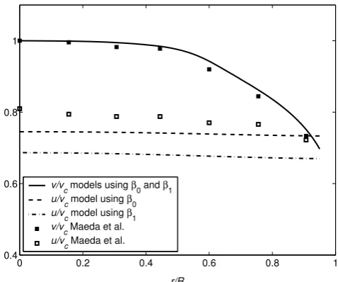
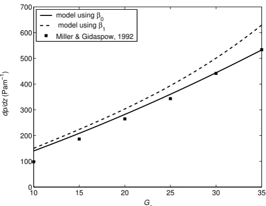
smaller slip velocity is predicted. This then leads to a lower axial pressure drop along the pipe, which can be seen in Figure 3. There is a negligible difference between profiles of normalised gas axial velocity calculated using β₀ and β₁.

Figure 3 compares the experimental data of Miller and Gidaspow (1992) with the simulation

. Conclusions

dels for gas-solid flows, the averaged drag force plays an essential role in

eferences

.B. & Jackson, R. (1967). Fluid mechanical description of fluidized beds:

Di interaction systems. Int. J.

Er hrough packed columns. Chem. Eng. Prog. 48, 89.

nd fluidised

Ho riels, W.J. & Van Swaaij, W.P.M. (1996). Discrete

results of the model of Neri and Gidaspow (2000) using β₁, and the present model using β₀. In the two simulations, all other model parameters apart from the momentum transfer coefficient are identical. The physical system examined is, again, vertical pipe flow, with a superficial gas velocity of 2.89 ms-1. The most evident impact of using the new β₀ is that the predicted axial pressure gradient becomes smaller. Simulation results using β₀ show better quantitative agreement with the experimental measurements in both Figures 2 and 3. This indicates that the validity and applicability of the new expression for β₀ for the inter-phase momentum transfer coefficient are worth further exploration.

5

In two-fluid mo

coupling the gas and particles. As this drag force has a considerable effect on predicted flow characteristics, it is important to use the most accurate available expressions. The averaged drag force needs not only to incorporate the influence of solid volume fraction but also to address the effect of the random fluctuational motion of the particles.

R

Anderson, T

comparison with theory and experiment. I&EC Fund. 6, 527. Felice, R. (1994). The voidage function for fluid-particle

Multiphase Flow 20, 153. gun, S. (1952). Fluid flow t

Ergun, S. & Orning, A.A. (1949). Fluid flow through randomly packed columns a beds. Ind. Eng. Chem. 41(6), 1179.

omans, B.P.B., Huipers, J.A.M., B

Kawaguchi, T., Tanaka, T. & Tsuji, Y. (1998). Numerical simulation of two-dimensional fluidized beds using the discrete element method (comparison between the two- and three-dimensional models). Powder Tech. 96, 129.

Kürten, H., Raasch, J. & Rumpf, H. (1966) Chem. Ing. Tech. 38, 941.

Louge, M.Y., Mastorakos, E. & Jenkins, J.K. (1991). The role of particle collisions in pneumatic transport. J. Fluid Mech. 231, 345.

Maeda, M., Hishida, K. & Furutani, T. (1980). Optical measurements of local gas and particle velocity in an upward flowing dilute gas-solid suspension. Polyphase Flow and Transport Technology, 211. Century 2-ETC, San Francisco.

Mikami, T., Kamiya, H. & Horio, M. (1998). Numerical simulation of cohesive powder behavior in a fluidized bed. Chem. Eng. Sci. 53, 1927.

Miller, A. & Gidaspow, D. (1992). Dense, vertical gas-solid flow in a pipe. AIChE J. 38, 1801.

Neri, A. & Gidaspow, D. (2000). Riser hydrodynamics: simulation using kinetic theory.

AIChE J. 46, 52.

Nieuwland, J.J., van Sint Annaland, M., Kuipers, J.A.M., van Swaaij, W.P.M. (1996) Hydrodynamic modelling of gas/particle flows in riser reactors. AIChE J 42, 1569.

Niven, R.K. (2002) Physical insight into the Ergun and Wen & Yu equations for fluid flow in packed and fluidised beds. Chem. Eng. Sci. 57, 527.

Wen, C.Y. & Yu, Y.H. (1966). A generalized method for predicting the minimum fluidization velocity. AIChE J. 12, 610.

Yasuna, J.A., Moyer, H. R., Elliott, S. & Sinclair, J.L. (1995). Quantitative predictions of gas-particle flow in a vertical pipe with particle-particle interactions. Powder Technol. 84, 23.

δV2

[image:8.595.173.439.101.308.2]

δV1

Figure 1 Schematic of the elemental volumes δV1 and δV2 in a freely-moving gas-solid flow; solid circles represent particles. The inner broken line represents the boundary of the characteristic volume element δV1, containing a single particle with local voidage ε1. The outer broken line represents the boundary of δV2, the elemental volume which contains statistically many freely-moving particles.

0 0.2 0.4 0.6 0.8 1 0.4

0.6 0.8 1

r/R v/v

c models using β0 and β1 u/v_c model using β

0 u/v

c model using β1 v/v

c Maeda et al. u/v

c Maeda et al.

[image:8.595.176.415.457.656.2]

10 15 20 25 30 35 0

100 200 300 400 500 600 700

G s

dp/dz

(Pam

−1

)

model using β

0

model using β

1

[image:9.595.168.428.133.334.2]

Miller & Gidaspow, 1992