Investigations in Gas-Solid Multiphase Flows

(1)

NEHAL N. DESAI. Investigations in Gas-Solid Multiphase Flows. (Under the direc-tion of Professor Kevin M. Lyons.)

(2)

by

Nehal Desai

A thesis submitted to the Graduate Faculty of North Carolina State University

in partial fulfillment of the requirements for the Degree of

Doctor of Philosophy

Mechanical Engineering

Raleigh 2003

APPROVED BY:

(3)

BIOGRAPHY

(4)

List of Figures

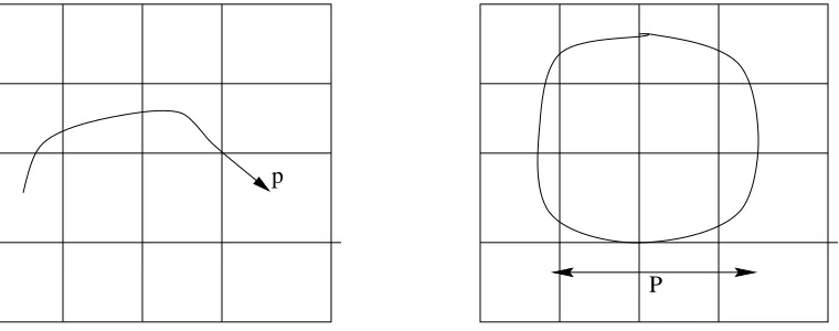
1.1 a. Point mass and b. Resolved volume . . . 11

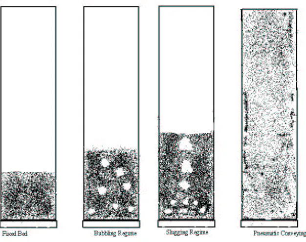
1.2 Transition points in a fluidized bed . . . 13

1.3 Evolution a bubble in a fluidized bed with obstacle. Increasing time from left to right. . . 15

1.4 Time Averaged solid void fraction at 3 locations. (a). Position 1 is 3 cm from the centerline (b). Position 2 is 10 cm from the centerline (c) Position is 17 cm from the centerline . . . 15

2.1 The virtual overlap of 2 particles . . . 28

2.2 Control volume . . . 52

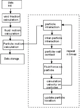
2.3 Lagrangian simulation flowchart . . . 61

2.4 (a) Mean air velocity distribution in the presence of 500µm at (a)m=0.0 (b) m=0.7 (c) m=2.5 . . . 64

2.5 Mean air velocity distribution in the presence of 200µm at (a) m=1.3 (b) m=3.0 . . . 65

2.6 500 µ m particle velocity distributions for different mass loading (a) m=1 (b) m=1.1, (c) m=3.1 . . . 66

3.1 Outline of the inverse algorithm . . . 76

3.2 Schematic of a fluidized bed . . . 77

3.3 Transition points in a fluidized bed . . . 78

3.4 Three types of viscous dissipation in a granular flow – kinetic,collisional and frictional . . . 84

3.5 Schematic of fluidized bed used in simulations . . . 99

(7)

List of Tables

1.1 Examples and categories of multiphase flow . . . 3 3.1 Abs. relative errors of initial guess A=.693,B=4.55,C=1.28,D=2.65 . 100 3.2 Abs. relative errors of initial guess A=.693,B=3.72,C=1.28,D=2.65 . 102 3.3 Abs. relative errors of initial guess A=.570,B=4.55,C=1.28,D=2.65 . 102 3.4 Abs. relative errors of initial guess A=.570,B=3.72,C=1.28,D=2.65 . 103 3.5 Abs. relative errors of initial guess A=.570,B=3.72 for clustered

con-figuration . . . 122 3.6 Abs. relative errors of initial guess A=.570,B=3.72 for random

(8)

Chapter 1

(9)

1.1 Introduction

Multiphase flows are encountered in many important engineering and environmen-tal systems. Because of there commercial importance understanding and improving multiphase processes has become an active area of research. To improve multiphase systems requires among other things a better understanding of the multiphase flow physics. One of the most important tools to improve our understanding of multi-phase flow is computer modeling. With recent advances in computer hardware and software, the ability to model complicated phenomena like multiphase flow has never been greater. However, multiphase flows are complex and correctly understanding the assumptions and limitation of the computer (and theoretical) models is vital to process optimization. This thesis re-examines many of the basic assumptions used in the computational and theoretical modeling of multiphase flow and aims to find alternate strategies and approaches that permits the modeling of these flow more effectively.

(10)

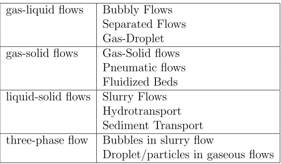
gas-liquid flows Bubbly Flows Separated Flows Gas-Droplet gas-solid flows Gas-Solid flows

Pneumatic flows Fluidized Beds liquid-solid flows Slurry Flows

Hydrotransport Sediment Transport three-phase flow Bubbles in slurry flow

Droplet/particles in gaseous flows

Table 1.1: Examples and categories of multiphase flow

Loth [41] is a comprehensive introduction to the numerical approaches used to model gas-solid flows. Crowe, Tsuji and Sommerfeld [17] is excellent introductory book to gas-solid flows. Many of the topics discussed in this introduction are given a fuller treatment in this book. Enwald, Pierano and Almstedt [28] discuss the application of Eulerian techniques to the fluidizing systems and give a complete derivation of two-fluid multiphase equation.

1.2 Gas-Solid Phase Overview

(11)

and dense gas flows. Though descriptive, the terms dilute and dense are ambiguous and give little insight into the flow physics or modeling approaches. In the next few sections we will

• Review criteria to determine the type of flow (dilute or dense).

• Review the impact of this categorization on modeling approaches.

1.2.1 Criteria for gas-solid flows

As stated previously, the key factors in determining whether a flow is dilute or dense is the type and magnitude of the interactions between phases. These interac-tions can be of two types: interaction between the constitutive elements of the solid phases (the interparticle interaction) and the interaction between the solid and fluid phases. The interaction between particles is further subdivided into: collisional in-teractions and hydrodynamic inin-teractions (lubrication inin-teractions). By comparing the various gas, solid, and collisional timescales, criteria have been established to determine the density (or relative density) of the multiphase flow. Loth [41] gives a number of interesting criteria for dilute flows. The most widely used measure of the gas-solid flow density is the mass loading, which is the ratio of the solid phase mass flux to the fluid phase mass flux.

Z = ρ¯pvp ¯ ρfvf

(12)

Here ¯ρp =npmp and ¯ρf = (1−nPV Cp)ρf. Using the well know relationship between

density,mass and volume and assuming that particles are spheres and can never exceed the total volume (npVp ≤1). We can get the relationship.

Z =

"

npVp

1₋(npVp)

# "

ρp

ρf

# "

vp

vf

#

(1.2)

Inaddition to establishing criteria for dilute and dense phase flows, timescale anal-ysis is useful in the determining the interactions of a single particle with the gas phase. The degree to which a particle maybe in kinetic equilibrium with the surrounding gas is given by the ratio of the particle timescale to the fluid timescale.

St = τp τf

(1.3)

The Stokes number dictates how readily a particle follows the flow. For laminar flows this relationship is straightforward.

St= npπρpdp|vf −vp|

18µ (1.4)

(13)

unity means that a particle acts as diffusive tracer and can quickly respond to fluc-tuates in the flows. For Stokes numbers greater than unity particles do not respond quickly to changes in the flow. Taken together, the mass loading and Stokes numbers portend one of the central issues/problems of gas-solid multiphase flows – phase cou-pling. Depending on how the phases interact, phase maybe coupled in three ways: mass coupled, momentum coupled and energy coupled. If the gas and solid particle exchange momentum they are said to be momentum coupled. Momentum coupling provides the vital link between mass loading, the Stokes number and the modeling approaches of the next section. In general

Πmom =

Z

(1 +St) (1.5)

which implies that momentum transfer (Πmom) increases with increased mass loading

(14)

1.2.2 Modeling approaches

Until recently, the type of computer model used to explore gas-solid flows de-pended on the ”density of flow” as defined by the mass loading or other flow met-rics [41]. Dense gas-solid flows like those in a fluidized catalytic cracker, were modeled by extending fluid continuum models,which assume that the primary characteristics of the multiphase system (void fraction, particle velocity, etc) could be described by continuum equations in a fixed or Eulerian reference frame. Dilute flows (low Z and low Πmom) were modeled using Lagrangian models,which treat the solid phase as

dis-crete particles that are individually tracked through the fluid phase. These methods are described in more detail below.

Eulerian Models

(15)

empirical or semi-empirical constitutive and transfer equations. In general two-fluid models seek to apply volume averaging [28] [62] [22] techniques to the instantaneous equations of motions for each phase. The result is a Navier-Stokes-like set of equations for each phase with additional closure equations. Implicit in the averaging process is the understanding that the interphase expressions are based on a point-volume description of the particle. Closure equations are of three types: constitutive, transfer and topological.

• Constitutive equations specify how the physical properties of the phases inter-act with one another other, but do not describe the mass, momentum or energy transfer between them. Examples of the physical parameters that can/are pre-dicted with the constitutive equation include: the viscous stress, particulate phase bulk and dynamic viscosity and particle pressure. Many constitutive equations are based on empirical models of particle properties and the void fraction. The most recent models use the kinetic theory of granular flows to develop many of the constitutive relationships [31].

(16)

• Topological equations are used to describe the spatial distribution of a flow variable.

The Eulerian approaches have a number of advantages over the Lagrangian approach. The primary one being less computational expense (for approximately the same type of problem). In general Lagrangian methods require that each particle and its as-sociated characteristics be stored during the calculations. It is easy to see that for even moderately dense flows the associated memory and computational requirements may be quite large. Because Eulerian methods are grid-based, memory and the com-putational requirements do not change radically with the introduction of additional particles. However, a number of problems exist with two-fluid models including: the type and nature of the boundary conditions for wall-bound flows, where the tangential particle velocity will not be zero as it is for the fluid phase; polydisperion of particle size and the sometimes dubious nature of the gas-solid and solid-solid momentum exchange terms. This last problem is addressed in more detail below in this thesis.

Lagrangian methods

(17)

influence the gas domain or its discretization. The point mass techniques are used to model large numbers of particles without regard to the specifics of the gas-solid fluid mechanics (e.g. boundary layer effects). In the point mass representation the trajectory of the particles through the gas phase is determined by integration of the particle equation of motion (PEM) which is based on the forces that are assumed

to act on the particle. If the particle diameter is larger than the grid spacing (we have a very fine grid), the resolved volume representation is used. Resolved volume approaches avoid the modeling assumptions present in the point mass representation (e.g. PEM) by discretizing the three dimensional particle flowfield. Thus producing a more detailed understanding of the gas flow around particles. However, this results in greater computational expense per particle, which makes the resolved volume method unsuitable for engineering applications where many particles must be modeled. The point mass and resolved volume representation can be thought as complimentary techniques. Often, resolved volume calculations are used to examine the assumptions of point mass techniques. According to Loth [41] strict application of the point mass method requires the particle diameter to be smaller than the characteristic microscale eddy length, which for turbulent flow is the Komologrov scale. Most turbulent flows of interest to engineers do no meet this criteria (e.g. dp ≤ λk).

(18)

p

P

Figure 1.1: a. Point mass and b. Resolved volume

terminal velocity of a particle in a quiescent fluid, the Reynolds Averaged Navier Stokes (RANS) method is unsatisfactory as there are no spatially resolved turbulent structure in these approaches. When RANS methods are used to calculate the gas phase velocities, a modification of the point mass method is used. The ”cell-averaged” point mass models the spatial and temporal turbulence within the grid cell in order to predict their influence on the particle momentum equation. In addition, the influence of the instantaneous velocity fluctuations at the particle must be modeled. How turbulent flows effect particle motion is described in excruciatingly detail by a number of authors.

1.3 Applications

(19)

transports and separations processes. Like many current research areas, the study of gas-solid flows emerged from a practical need to understand commercial processes. Perhaps because of this genesis much of the research in gas-solid flows is in framed in terms of benchmark applications like the fluidized catalytic crackers and pneumatic transport. In addition to their commercial value, these systems have interesting hy-drodynamics properties, which often are the same properties that make/made it an commercially important. In the next section, the hydrodynamics of multiphase flows is examined in the context of these applications. The purpose of examining these applications in detail is to 1). Provide motivation to the rest of the study 2). Provide a reference framework for later discussions 3). Provide an introduction to the wide range of hydrodynamic phenomena produced by multiphase flows.

1.3.1 The Fluidized Catalytic Cracker

(20)

Figure 1.2: Transition points in a fluidized bed

(21)

has proven a difficult challenge for the experimentalist as well as the theorist. Seg-regation is the migration of small or light particles upward while the heavy particle travel downward in a bubbling fluidized bed.

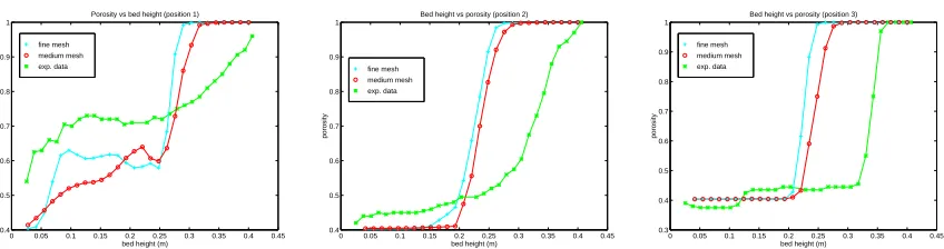
Fluidized beds are prime examples of a dense phase flow, in which particle-particle collisions are the primary mechanism for interphase mass transport. Fluidized beds are one of the primary applications used to benchmark two-fluid Eulerian models, although a few researchers have attempted to use Lagrangian methods (or one its variations) to model fluidized bed system. Perhaps the hardest hydrodynamics feature of the fluidized bed for most current model to capture is bubbling. The figures below show the results of a typical fluidized bed bubbling calculation. The air enters the bed through a single opening (1.37 cm OD) at the centerline (below the obstacle) at a velocity of 5.77 m/s. The bed material is composed of 880µ m particles with a density of 2.42 g/cm3_{. The bed is 20 cm from the centerline to the wall. The}

simulation time was 1.5 seconds. The figures below show the rise of a single bubble in a fluidized bed with an immersed obstacle. The figures show the time evolution of solids volume fraction as bubble rises through the FCC. The darker regions have a higher solids concentration. Figure 1.3.1 shows the time-averaged air fractions (²f)

at 3 locations in the bed.

(22)

Figure 1.3: Evolution a bubble in a fluidized bed with obstacle. Increasing time from left to right.

fine mesh medium mesh exp. data

0 0.05 0.1 0.15 0.2 0.25 0.3 0.35 0.4 0.45 0.4 0.5 0.6 0.7 0.8 0.9 1

bed height (m)

porosity

Porosity vs bed height (position 1)

0 0.05 0.1 0.15 0.2 0.25 0.3 0.35 0.4 0.45 0.4 0.5 0.6 0.7 0.8 0.9 1

bed height (m)

porosity

Bed height vs porosity (position 2)

0 0.05 0.1 0.15 0.2 0.25 0.3 0.35 0.4 0.45 0.3 0.4 0.5 0.6 0.7 0.8 0.9 1

bed height (m)

porosity

Bed height vs porosity (position 3)

Figure 1.4: Time Averaged solid void fraction at 3 locations. (a). Position 1 is 3 cm from the centerline (b). Position 2 is 10 cm from the centerline (c) Position is 17 cm from the centerline

more sophisticated understanding of the physics involved.

1.3.2 Pneumatic Transport

(23)

multi-phase flows. A typical pneumatic particles in pipe (PIP) experiment is shown below. A number of experiments have been done which study the flow of air and particle in pipe. Tsuji [71] [70] examined both the horizontal and vertical piping systems. The experiments for vertical pipe reveal a number of interesting phenomena including a skewing of the maximum gas velocity. For single phase mildly turbulent pipe flow, the maximum velocity is at the centerline of the pipe, however for gas-solid flow at moderate mass loading (ml=2.1-3.1), the maximum velocity shifts away from center. As the loading increases the gas phase velocity shifts further away from the center. Durst and Lee also conducted a series of experiments in which they measured the particle and gas-phase velocity of several different size particles and different mass loading.

1.4 Purpose and motivation for this study

(24)

1.4.1 Application of inverse theory to two-fluid multiphase

flows

The first idea explored in this thesis is the use of inverse theory to determine momentum closure relationships. The momentum relationships are key to under-standing the physics of multiphase flow, but more importantly they are the key to understanding (and therefore optimizing) the operational behavior of processes that use gas-solid flows (e.g.FCC and pneumatic transport). As discussed above, the mo-mentum closure relationship or momo-mentum exchange terms (MET) are used in two fluid modeling to couple the solid and gas phase momentum equations and in some models couple the solid-solid momentum exchanges [52]. Often these relationships or terms are based on dubious assumptions about the nature of the solid gas interaction (e.g. single particle dynamics). The drag correlations derived from these assumptions are often empirical relationships that depends on a few factors including: solid parti-cle diameterdp, particle densityρp, the void fractions of the solid and gas phases, ²s

and ²g, the particle Reynolds number and the velocity difference between the phases

|Vs−Vg|. For example Symlal and O’Brien derive the following formula for gas-solid

interaction.

Fsg =

3²g²sρg

4V2

rmdp

(6.3 + 4.8qVrm/Rep)2(Vs−Vg) (1.6)

and

(25)

where Vrm is the ratio of the terminal velocity of a group of particle to a single

isolated particle, and Rep = dp|Vs −Vg|ρg/µg is the solid phase particle Reynolds

number. Now the question arises, can you successfully model multiphase phenomena with so little ability to change the interaction of the solid and gas phases. As it stands, the only operational parameters which differentiate a fluidized bed of sand and a fluidized bed of reactive catalyst are the particles’ diameter and density. Is this a plausible assumption given the complex flow phenomena experimental observed? We seek to answer this question (or some part of it) by examining the results of an inverse parameter estimation study. In this study, the MET is parameterized and than estimated from a combination of experimental data and computational modeling. Traditionally, inverse methods have been applied to complex phenomena where the object is to extract vital process or operational information (e.g. oil or strength of material). This is precisely the type of information that would allow operational optimization of multiphase flows. Because inverse methods require experimental a short and related discussion is given of information theoretic methods for design of experiment. Though only tangentially important to the physics of multiphase flows, proper design of experiment is vitally important to most engineers.

1.4.2 The Lagrangian method for dense multiphase flows

(26)

solid and gas phases and the great computational expense of running simulations with large numbers of particles. Until recently the latter constraint limited these types of simulation to the largest computers. However, with the advent of faster microprocessors, large dense phase Lagrangian simulations have become viable for cluster is of desktop machines. The second part of this thesis examines the use of a mixed numerical scheme; Eulerian gas flow with Lagrangian particles tracking for dense solid-gas flows. The results of the simulation are compared against the experimental results of Tsuji [71] and Durst and Lee [39]. Few computational schemes have been able to reproduce the general trends in Tsuji and Durst and Lee’s work.

1.4.3 Conclusion

(27)

Chapter 2 Euler-Lagrangian for dense phase

(28)

2.1 Introduction

A number of industrial processes involve the flow of particulate materials. Ex-amples include: pneumatic conveying, flow in the riser section of a fluidized bed reactor,polymer processing and stirred tank mixing. Because a clear understand-ing of the physical mechanisms in these flows is vital to scale-up and design of new processing equipment a great deal of numerical and experimental research has been conducted in this field. Most computer simulations of gas/solid flows can be divided into two categories: Eulerian (continuum) models and Lagrangian models. Eulerian models seek to derive a set of continuum equations in each phase by application of averaging techniques to the instantaneous equations of motion in each phase [28]. The averaging procedure used to obtain the continuum equations also produces a number of ancillary dependences that must be resolved before proper closure of the equa-tion set. These ancillary relaequa-tionships and the accompanying constitutive equaequa-tions make the application and interpretation of two fluid models difficult. An alternative to continuum models, and the approach taken in this study, is to use Lagrangian methods.

(29)

cou-pled formulation in which the influence of the particles on the fluid phase is taken into account by introducing source terms into the Eulerian fluid equations,thereby coupling the phases. This formulation is important at higher mass loading, where the presence of the solid phase influences the gas phase and visa versa. In the second category, the flow’s fluid dynamics determine the particle distribution. Often called one-way coupling, this method is used to model systems in which the mass loading is low (i.e. particle flow interaction are minimal).

Lagrangian methods have a number of advantages over continuum models such as the simplified modeling of multi-size particles and fewer assumptions about the equations. But until recently, the computational expense of Lagrangian methods meant that only a small number of particles could be tracked, severely limiting the applicability of these methods to industrial flows. However, the advent of high-speed multi-processors computers now make Lagrangian simulation a viable alternative to two-fluid models in the dilute to moderately dense phases regimes. This study reports on efforts to understand gas/particle flows through a two-way coupled simulation, the results of which are compared against experimental results. Special emphasis has been placed on computational efficiency and algorithmic generality in order to produce a stable framework in which to conduct these numerical experiments.

(30)

Lagrangian particle methods have been used to study various aspects of gas-solid flows including: particle-fluid turbulence interactions [46] [27] hydrodynamic forces between the solid and fluid phases [44], and particle-particle interactions [72] in dense flow systems. Lun and Liu [42] modeled the flow of particles in horizontal channel coupling the particle and fluid momentum. In the next two sections, we examine the hydrodynamic and collisional interactions of solid particle in a fluid stream.

2.2 The particle equation

In its most general form the equation governing particle motion is:

mp

dup

dt =ΣFp (2.1)

where up is the velocity of the particle and ΣFp is the sum of the forces on the

(31)

a sphere in a quiescent fluid serves as the basis for the hydrodynamics forces. How-ever, because of the assumptions used in its derivation, the Maxey-Riley expression must be modified and augmented in order to be valid in the flow regimes of interest. Particle-particle interactions become increasingly important as the mass loading (or the particle concentration) increases. With higher mass loading the average time be-tween particle collision is smaller than the average time the particle spends bebe-tween collisions. Thus the particle has little time to responds to the hydrodynamic forces. Particle-particle interactions also prevent particle concentrations from exceeding the maximum concentration for the physical properties of the particle. The particle equa-tion used in the study is of the form:

mp

dup

dt =Fd+Fl+Fvm+Fpg+Fwall+Fcoll+ (1− ρf

ρp

)g (2.2)

WhereF_dis the drag forces, F_l are the lift forces,F_vm is the virtual mass force,F_pg is the pressure gradient force,Fwall is the wall interaction force andFcoll is the collisional

(32)

2.2.1 Hydrodynamic forces

Drag

Drag is felt by objects as they move through the fluid and is a result of pressure and frictional forces on the objects surface.

Fd =

1 8Cdπd

2

pρf(uf −up)|uf −up| (2.3)

Here, Cd is the drag coefficient. The general form of the drag coefficient for a

sphere [50] is

Cd=

K1

Rep

+ K2 Re2

p

+K3 (2.4)

where K1, K2 and K3 are empirically derived coefficients.

Lift

Lift forces, which act perpendicular to the drag forces, has two principal compo-nents. The Saffman lift (Fls)due to fluid shearing and the Magnus lift (Flm) due to

asymmetric flow

The Saffman lift force is:

Fls= 1.615Csm(ρfµf)1/2d2p|ωf|1/2[(uf −up)×ωf] (2.5)

(33)

in which both the particle Reynolds number, Rep and the Reynolds shear number,

Resh(=d2p/νduf/duy) are less than one. For Rep >40; Csm =.0524(Rep_2|_udp

f−up||ωf|).

Implicit in this form of the Saffman lift forces is the assumption that the distance from the particle to the wall is much greater than the particle radius. This assumption plays an important role in the scaling analysis to follow.

The Magnus lift forces is due to asymmetric flow around the particle

Fm =

1

2ρf(uf−up)

2πd 2 p

4 CLM

(uf −up)× ωr

|ωr|

(2.6)

CLM is the lift coefficient and has an approximate value of .5 for dilute suspensions.

The spin of the particle relative to fluid

ωr =∇ ×up−.5∇ ×uf (2.7)

Virtual Mass Force

When a body is accelerated through a fluid there is an acceleration of the fluid around it. The additional force required to accelerate this fluid is called the virtual mass force. Auton [5] gives the virtual mass force as

Fvm =

ρf

2Vp

d

(34)

Pressure gradient forces

The pressure gradient force is

Fpg =ρf

Duf

Dt (2.9)

where: D

Dt is the material derivative = ∂

∂t +uf · ∇

2.2.2 Interparticle force

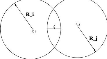
In general, there are two techniques employed for modeling particle-particle inter-actions in gas-solid flows. The first is the hard sphere model, which is based on the impulsive forces between particles, and the soft sphere model, in which the amount of ”overlap” between particles is used to produce a repulsive force [17] [59]. In this study we use the soft sphere model, because of its simplicity and easy of implementation. In the soft sphere model, the interparticle force,Fcoll is composed of a normal and a

tangential force.

Fcoll =Fcolln +Fcollt (2.10)

The normal component of the collisional force is of the form

Fn

coll = (−knζij−λn(vi−vj)nij)nij (2.11)

(35)

ζij =dp− |xi−xj|,xi is the (x,y,z) coordinate of the center of mass for particle i (or

j),nij is the unit normal pointing from particle i to particle j andλn is the dissipative

constant. The stiffness constant,kn is calculated from Hertizan contact theory [69],

R_i

ζ

X_i

X_j

R_j

Figure 2.1: The virtual overlap of 2 particles

in which Poisson’s ratio,σ2

s and Young’s modulus,Es determine the ”strength” of the

contact between the two particles. According to this theory, the normal component of the collisional force,Pn and the virtual overlap ζij are nonlinearly related

Pn=Knζij3/2 (2.12)

In the case of two sphere of equal diameter

Kn =

q

2dpEs

3(1₋σ2

s)

(2.13)

Substitution of the Hertizan contact force,Pn into the equation 2.11

Fn_coll = (₋Knζ 3

2 −λ

(36)

The dissipative constant,λncan be derived from the critical damping condition of the

spring-dashpot-friction slider mechanical system. Tsuji has extended this model by relating the dissipative constant to the materials coefficient of restitution, ²p.

λn =β(²p)

s

mp

Pn

ζij

(2.15)

where β is a function of the restitution coefficient (²p). For the particles used in this

studyβ=.2 (²p=.8). The tangential component is of the form:

Ft_coll =₋fFn_coll nij

|nij|

(2.16)

fis the friction coefficient, which is a measurable quantity.

2.2.3 Wall-particle interactions

(37)

term, which in its original form does not include the wall effects. These modification still assume that l _¿ dp, where l is the distance between the particle center and

the wall. The second mechanism for wall particle interaction is mechanical behavior. Depending its inertia, a particle may collide with the wall or be captured with cohesive force (eg. van der Waals forces). The collision between wall and particle can be modeled with either the hard sphere or soft sphere approach.

2.2.4 Scaling and Non-Dimensional Groups

Scale analysis of the governing equations and hydrodynamics forces provides con-siderable insight into the behavior (eg. timescale) of the flow. Assume typical values for the parameters in solid/air vertical pipe flow [39] [71]: are: dp=.03m,ρf ≈1.2_mkg3,

νf ≈ 1.5e− 5m

2

sec, dp ≈ 5e −4m, ρp ≈ 2000kg/m

3_, _λ ₌ up

uf. mp ≈ 5.5e −7kg ,

Ap ≈2.01337e−6m2 thanFd≈3πνfdpρf|uf(1−λ)|+1.413ν.313d1p.687ρf|uf(1−λ)|1.687.

It becomes clear that the importance of the Saffman and drag forces are dependent on two factors: the difference between the particle and fluid velocities (uf(1−λ)) and

the rate of shear (_|duf/dy|). The following criteria must be met for the Saffman and

drag forces to be of the same order of magnitude:

2432[uf(1−λ)] + 6650[uf(1−λ)].628 ≈ |duf/dy| (2.17)

(38)

relative velocities are small and the shear rate maximum, the issue of whether the criteria above can be met is not so clear. Thus, inclusion of the Saffman lift into the reduced particle equation is problematic. The issue is complicated by the lack of experimental data close to the wall. Based on these factors the Saffman force is not included in the study.

The pressure gradient force, Fpg ≈ρf/ρp ≈10−3 and is negligible.

The gravity term, mg _≈ 5.4e₋6 is an order of magnitude less than the drag force, but because drag scales as the velocity squared, at lower relative velocities the gravity would be of the same order (or larger) than the drag, and therefore must be included in the final form of the particle equation. The particle equation (1) can now be simplified

mp

dup

dt =Fd+ mpg+Fcoll (2.18) The virtual force and Bassett forces are negligible because ρf/ρp ≈10−3.

In addition to simplifying equation 2.2, scaling analysis aids in the effort to es-tablish parameters that characterize particle motion. For turbulent flow systems, particulate motion depends on a number of factors including: the Stokes number (St), defined as

St = τp τf

(2.19)

(39)

fluid timescale. If the Stokes number St _¿ 1 than the particles can be expected to follow the flow, similarly for St_À1 the particle are not influenced by the turbulent flow structure, having insufficient time to response to the fluid fluctuations. The particle timescale scales as , τp ≈ ρpd2p/18µ ≈ 4.7s. The fluid timescale is more

complicated. A number of fluid timescales can chosen including: viscous, Kolmogorov and large eddy. In pipe flow, the large eddy timescale maybe the most appropriate for the calculation of the Stokes number [25]. Assumingτf = 0.003s, St≈1500, implying

that turbulence does not influence the particles trajectory through the flow. If the viscous timescale is chosen, the Stokes number calculated becomes a measure of the influence of non-homogeneities close to wall on the particle. Young and Hanratty [74] claim that for a viscous Stokes number, St_≥ 20-30 wall turbulence is not important. Assuming a viscous timescale, St _≈ 100000, implying that wall bound turbulence is not important.

2.3 Fluid Equations

(40)

of textbooks and journal articles that cover almost all aspects of the Navier-Stokes including: the numerical techniques that are used to solve the various forms (com-pressible,incompressible,turbulent etc) of the Navier-Stokes. In the next sections we will review the Navier-Stokes, the influence of turbulence on particle dispersion and finally the incorporation of turbulence into the Navier-Stokes Equation.

2.3.1 The Navier-Stokes Equation

To review: the Navier-Stokes equations (in the x,y,z coordinate system) are of the form: 1. Mass Conservation Equation

∂

∂t(ρf) +∇ ·(ρfuf) = 0 (2.20) 2. Momentum Conservation Equation

ρf[

∂

∂t(uf) + (uf∇)uf] = dP

(41)

2.3.2 Interaction of turbulent flow with solid particles

In this section we will review the effect of turbulence on solid particles. Although, we have concluded from the scaling argument above that the effect of turbulence is relatively minor (given the large Stokes number) for the particles and flows speeds in this study, how turbulence effects small particle (St _≤ 1) dispersion is an important topic and should be reviewed. Shirolkar, Coimbra and McQuay [61] is an excellent review of turbulence and its effect on solid particles. Much of the discussion below is taken from this reference.

Turbulence is the three dimensional macroscopic manifestation of increased vor-ticity and strain in the flow. Researchers in the area turbulent flows have devised a number of conceptual frameworks in order to understand turbulence. The most widely applied framework uses the concept of an eddy (or the rotating structures found in turbulent flow) to understand how turbulence is generated, how scalar quantities are transported in turbulent flows and how turbulent flows interact with solid objects (e.g. solid particles). This model has a number of assumptions which help to understand and model turbulent flow and its interactions with solid particles including:

1. Eddies of various sizes are present in a turbulent flows.

2. Because large eddies cannot respond to rapidly to viscous forces they are often broken into smaller eddies. This phenomena is called turbulence decay.

(42)

4. Each eddy has an associated length and timescale known as the eddy length and the eddy lifetime. The eddy length is the physical size of the eddy and eddy lifetime is the time that eddy will maintain its current size.

With the ”basic” assumptions out of the way, we can now go on to the more complex issue of the interaction of solid particles and turbulent eddies. The interaction of the solid particle and a turbulent eddy depends on two factors: the inertia of particle and the particle’s free velocity. The influence of a particles’ inertia was discussed briefly in the last chapter. Infact our discussion of the Stokes numbers was really a discussion of the effects of inertia on particle-eddy interactions (though we didn’t frame the argument in terms of inertia explicitly). The second factor effecting a solid-particle eddy interactions is the particle’s free fall velocity or terminal velocity, which is an important in the migration of particles from one turbulent eddy (before it decay due to viscous forces) to another eddy. The so-called crossing trajectory effect (CTE) is an important (experimentally verified) feature of turbulent particle flows.

Lagrangian Particle Dispersion Models

(43)

flow. The variance in the fluid particle position (σ2

x) in one dimension is given as

σ2_x= 2

Z t1

0

Z t2

0 h(u 0

p(t2)u0p(t1))idt1dt2 (2.22)

Where u0

p is the fluctuating part of the particle velocity (more on the this later. For

right now assume that a particle’s velocity is the sum of a steady velocity, _hupi and

a fluctuating velocity u0

p). In order to avoid the problem of estimating the velocity

autocorrelation, _h(u0

p(t2), u0p(t1))i Taylor defined an autocorrelation function that is

a function of the time difference (ξ=t1-t2).

RL(ξ) = hup(0)up(ξ)i

hu2

pi

(2.23)

Substituting (2.23) into 2.22 and simplifying with partial fractions yields:

σ_x2 = 2_hu0_i2

Z t

0 (t−ξ)R

L_(ξ)dξ _(2.24)

If we assume a very form for the autocorrelation:

R=         

1.0, ξ < tf l

0, otherwise

(2.25)

(44)

over which the fluid is correlated with itself.

tf l =

Z t

∞R

L_(ξ)dξ _(2.26)

More intuitively, it can be viewed as the characteristic large eddy lifetime.

Using the Venkatram autocorrelation(2.25) function, we are able to derive two important results. Firstly, if the travel time of the particle is less than the Lagrangian timescaletf l the variance of the fluid particle grows as the square of the time of travel.

σx2 =hu0i2t2 (2.27)

When the particle travel time is much less than the Lagrangian fluid time scale, the variance become proportional to the time of travel.

σ_x2 =_hu0_i2tf l (2.28)

(45)

probability to transition between states [34]. A short explanation of each model is given below.

Random Walk Models

In the random walk model, a particle’s trajectory is defined by two equations;

dy=u0_p(t)dt (2.29)

and

u0_p(t+dt) = RL(dt)u0_p(t) +RWp (2.30)

RWp is a normal random variable that can be sampled from a Gaussian probability

density function. Equation 2.30 is the finite difference form of the Langevin equation. It can be shown that as dt approaches zero, the autocorrelation function assumes a exponential shape. Thus we are able to validate random walk models with the Taylor’s model by using an exponential autocorrelation function,RL₌_e(_|_ξ/t

f l).

Deterministic Dispersion Models

In these type of model the fluctuating component of the of the particle velocity u0

p is modeled as

u0p = Λp

1 ¯ np

∂n¯p

(46)

here Λp is the particle diffusivity which is the ratio of the turbulent particle viscosity

and the turbulent particle Schmidt number. Obviously, this methods suffers from the same parameter estimation problems that the two fluid or continuum methods have.

Eddy lifetime Models

Eddy lifetime models estimate the fluctuating component of the fluid velocity (which is then used to estimate the particle velocity) by randomly sampling from a PDF generate from the local turbulence properties, k and ². For isotropic flows:

P(u0_f) =

s

3 4kπexp



−

u0

f2

.75k



 (2.32)

The fluctuating velocity associated with an eddy is assumed to be constant over the interaction time,τi. Knowing the interaction time and the u0f we can use

up =uf + (uoldp −uf)e−τi/tp+gtp[1−e−τi/tp] (2.33)

Generally, the interaction time,τi is

τi =min(tf l, tc) (2.34)

(47)

are also very good at modeling the crossing trajectory effects (discussed previously).

Time-correlated dispersion models

8 Time correlated dispersion models are similar to eddy lifetime models with that the fluctuating component of the fluid velocity along the particle path now calculated using its value at the fluid particle location and a spatial autocorrelation functions. Unfortunately, even the simplest details of these methods are very complex and the read is referred to works by Berlemont [8] and Burry and Bergeles [21].

PDF propagation models

In PDF propagation model, a PDF represents a group of particles having the same physical properties and initial condition. The particle statistics are extracted from this PDF. In most models of this type, the PDF is assumed to have a Gaussian distribution of the form:

p(x, y, t) = 1 2πσx(t)σy(t)

q

(1₋r2_(t))exp−

1

2(1₋r2_(t)) (2.35)

x₋νx(t)2

σ2

x(t) −

2r(t)(x−νx(t))(y−νy(t)) σx(t)σy(t)

y₋ny(t)2

σ2

y(t)

(2.36)

where: r(t) = σxy

σx σy, νx is the ensemble mean particle location andσij is the particle

covariance relationship (which can be related to RL _{the particle correlation tensor.}

(48)

In reviewing the theoretical foundation of the most recent models for particle-turbulence it becomes clears that this issue is still a very active and potentially fruitful area of research. In the author’s opinion, many of the models shown (in spite of there complexity) lack a firm foundation. A more rigorous first principles approach (perhaps starting from statistical mechanics) may provide additional insight into the problem of solid particle-turbulence interaction.

2.4 Numerical Methods

In the previous section, we examined the effect of turbulence on small particle dispersion. As we noted previously, for the particles and flows under consideration turbulence is of secondary importance. But secondary importance does not mean of no importance, and we must take great care in selecting a turbulence modeling approach which works on both a theoretical and practical (implementation) level. Bardina [6] divides the techniques for predicting turbulent flows into six categories.

1. Correlations.

2. Integral equations.

3. One point closure models.

4. Two point closure models.

(49)

6. Direct numerical simulation.

The most commonly used technique to model turbulent flow are point closure models. The most common type of one point closure model is the Reynolds Averaged Navier-Stokes. The RANS techniques is ubiquitous and used in a number of commercial packages. In this approach the fluid velocity are divided into two parts: steady and unsteady, this ”new velocity” is substituted back into the Navier-Stokes and then averaged. The resulting equations require an additional set of equation to close the equation set. In the next sections, we will review how the Navier-Stokes equations are averaged, and the RANS equations constructed.

2.4.1 Preliminaries

In this approach the fluid velocities are first divided into two components a steady and two components a steady and an unsteady component.

uf = ¯uf +u0f (2.37)

where ¯uf is the steady fluid velocity and u0f is the unsteady component of velocity.

Equation 2.37 is then substituted into the governing equations and averaged. The averaging function is defined

¯

φ= lim

T→∞

1 T

Z T

(50)

Because equation 2.38 is a linear operator, its application to linear terms is straightfor-ward. For example if equations 2.37 and 2.38 are applied to the diffusive momentum term,_∇(_{∇ ·}u) the resulting equation _∇(_{∇ ·}¯u) has exactly the same form as the non-averaged equation. Only how the equation is interpreted changes. However, when 2.37 and 2.38 are applied to a nonlinear equation (eg. convective scalar flux) the resulting averaged equation has additional terms. The additional terms generated by the averaging procedure are problematic and require additional equations in order to ’close’ the equation set. To illustrate how averaging a nonlinear expression may produce additional terms a quadratic term is averaged.

ufφ = (¯uf +u0f)( ¯φ+φ0) (2.39)

(¯uf +u0f)( ¯φ+φ0) = (¯ufφ) + (¯¯ ufφ0) + (u0fφ) + (u¯ 0fφ0) (2.40)

Now, 2.40 is averaged.

(¯ufφ) + (¯¯ ufφ0) + (u0fφ) + (u¯ 0fφ0) = (¯ufφ) + (u¯ 0fφ0) (2.41)

Just to clarify, the simplification above, let’s review some of the properties of the average function and make clear the some of the assumption used. We assume that the average of the fluctuating component is zero ( ¯φ0 _{= 0). The last term on the right}

hand side is zero only whenu0

(51)

turbulent scalar flux. In the RANS momentum equations, when φ0 _{is equal to} _v0

f, the

resulting term (v0

fu0f) is called the Reynolds stresses. The Reynolds stresses are the

heart of RANS modeling and are the source of the ”closure problem” in turbulence modeling. In the RANS model the Reynolds stress terms can take two forms: the eddy viscosity model and the Reynolds stress model. Eddy viscosity models relate the Reynolds stresses (v0

fu0f) to the mean velocity gradients and a mean turbulent

dif-fusion (µt). Eddy models are classified by the number of partial differential equations

which must be solved in order to compute the turbulent diffusion. Zero equation (or algebraic models) compute the turbulent diffusion directly from the local mean flow quantities. Examples of algebraic models are the Prandtl mixing length model and constant viscosity models.

In two equation models like the k-ω and k-², two additional partial differential equations are required to close the Navier-Stokes. Reynolds stress models avoid the turbulent stress tensor terms by using individual equations for the individual turbu-lent stresses. Reynolds stress models use separate transport equations for each tensor component

2.4.2 The Reynolds averaged Navier-Stokes equations

(52)

volume fraction, β. All the quantities below are time-averaged. Only the fluctuation component is shown. The time-averaged continuity equation:

∂

∂t(βfρf) + ∂ ∂xi

(βfρfuf) = 0 (2.42)

The time-averaged momentum equation:

∂

∂t(βfρfuf) + (uf · ∇)(βfuf) = ∇ ·[µf(τij+τ

0

ij)] +βfρfg+Sp (2.43)

βf = (1−npVp/Vf). Equation (2.43) has the same form as the standard momentum

equations with the velocities now representing time-averaged values and the incor-poration of turbulence through the ”Reynolds-stresses”, τ0

ij. The mean fluid stress

tensor is:

τij=µ(∇uf +∇utf) (2.44)

and the Reynolds stress tensor is :

τ_ij0 =₋2

3ρfkδij+µt(∇uf +∇u

t

f) (2.45)

(53)

velocity and length scales.

µt=ρfCµ

k2

² (2.46)

The values of the k and ² are obtained by solution of the following conservation equations:

∂

∂t(ρfk) +∇ ·(ρfkuf) =∇ ·

µ

(µt σk

)_∇k

¶

+ Rk−ρf² (2.47)

∂

∂t(ρf²) +∇ ·(ρfuf²) =∇ ·

µµ

t

σ²∇

²

¶

+ C1Rk

²

k −ρfC2 ²2

k (2.48)

where Rk is the rate of turbulent kinetic energy production

Rk =µt(∇uf +∇utf)∇uf (2.49)

C1, C2, Cµ, σk and σ² are empirical constants with values of 1.44, 1.92, .09,.1.0,1.3

(54)

2.4.3 Momentum Exchange between Phases

The one of the most difficult problems in multiphase flow is understanding how non-collisional momentum is transferred between phases. This momentum transfer for sufficiently dense flows couples the phases. It is this coupling that produces the interesting hydrodynamics of the fluidized bed. As stated above, one of the factors that motivates the use of particle simulations for dense gas/solid flows is that momentum exchanges reveals itself more naturally as a byproduct of the drag and lift forces, rather then a explicit term in the Navier-Stokes equations. There are a number ways in which to couple the gas and solid phases, one of the most popular being the particle source in cell (PSI-cell)method [19].

SP SI−cell =

npmp

Vc

∆V

∆T (2.50)

Here ∆V is the change in velocity of particle between the entrance to a control volume and its exit, and ∆T is the time takes the particle to travel through the control volume.

2.4.4 Finite Volume Method

(55)

do-main of the differential equation is subdivided into a finite number of control volumes surrounding a grid point. The differential equation is integrated over each control volume producing a set of algebraic equations connecting the independent variable(s) (or scalar variables in the case of the generalized transport equation) and grid points. As the number of grid points increases, the finite volume method approaches the analytic solution.

According to Patanker [67] the most attractive feature of the finite volume method is that solution of the derived discretized equations imply a integral conservation of quantities such as mass,momentum and energy over any group of control volumes. In the next few sections the discretization process for a generalized transport equation is illustrated. The goal is to familiarize the reader with the basic concept of the finite volume methods, which will later be applied to the more complex Reynolds Averaged Navier-Stokes.

2.4.5 The general transport equation

Assume a conservation equation of the form

∇ ·(ρuφ) =_{∇ ·}(Γ_∇φ) + Sφ (2.51)

(56)

into a finite number of small control volumes. As the geometry of the solution do-main becomes more complex; how that dodo-main is discretized becomes increasingly important. In the finite volume method, the integral form of equation 2.1 is generally used as the starting point for the discretization of the governing equation. We begin the finite volume formulation by integrating Equation 2.51 over a generalized control volume:

Z

V ∇ ·(ρuφ)dV =

Z

V∇ ·(Γ∇φ)dV +

Z

VSφ (2.52)

A general method for the approximation of the spatial integral terms in the scalar transport equation (2.52) is outlined below:

1. The volume integral is converted to surface integral by application of the diver-gence equation

Z

V ∇ ·fdV =

Z

Sf ·ndS (2.53)

2. The surface integral is the sum of the integrals over each face,k of the control volume.

Z

Sf ·ndS =

X

k

Z

Sk

f _·ndSk (2.54)

(57)

Transient term

Integrating the transient term over a control volume leads to the approximation

Z t+δt

t

Z

V

∂(ρφ)

∂t dV dt (2.55)

If the control volume,V does not change in time the order operation of the integral can be changed and V can be neglected.

Z t+δt

t

∂(ρφ)

∂t dt (2.56)

There are several methods to approximate (or discretized) the time derivative. In general the time discretization can be divided into two categories: explicit discretiza-tion and implicit discretizadiscretiza-tion. The key difference between the two categories is the stability criterion or the rate at which the system is allowed to progress in time. Generally, implicit schemes allow larger time stepping and evolve the system faster.

Convective Term

The convective term is:

Fc =

Z

(58)

using the methodology outline above. The convective flux through the kth face is

F_kc =

Z

Sk

ρφu_·ndSk≈mkφk (2.58)

where mk is the mass flux through the ’kth’ face of the control volume. Because

the faces of the control volume lie between computational nodes (or nodes where values are known) interpolation must be used to approximate their values. Numerous interpolation schemes are available; two of the most popular schemes are linear (CDS) and upwind(UDS). How interpolation is used in the approximation of the convective flux is shown in the illustrated example below.

Diffusive Term

The diffusive term is

Fd=

Z

V ∇ ·(Γ∇φ)dV (2.59)

Using the methodology outlined above the diffusive convective through the ’k’ face can be approximated

F_kd=

Z

Sk

Γ_∇(φ)_·ndSk ≈Γ

Ã

∂φ ∂n

!

k

(2.60)

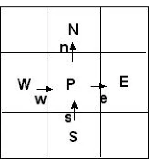
2.4.6 Illustrated example in 2-D

(59)

Figure 2.2: Control volume

The convective and diffusive fluxes can be approximated through any of the faces of the control volume. For illustrative purposes assume that we are interested in the ’e’ face of the control volume. The other faces can be integrated in a similar manner.

F_ec =

Z

Sk

ρφu_·n _≈meφe (2.61)

where me is the mass flux through the ’e’ face.

me = (ρux)e∆y (2.62)

(60)

interpolation the convective flux becomes:

F_ec =



   

   

max(me,0)φP +min(me,0)φE, U DS

me(1−λe)φP +meλeφE CDS

(2.63)

λe =xe−xP/xE −xP. The UDS approximation satisfies the boundness criteria

unconditionally, that is they never yield oscillatory solutions,however they are numer-ically diffusive,meaning that areas in which variables change rapidly will be smeared out. CDS schemes can yield oscillatory solutions but is the simplest second order scheme.

The diffusive flux is evaluated with CDS interpolation of the normal derivative;

F_ed= Γ

Ã

∂φ ∂n

!

e

∆y=Ad_e(φE −φP) (2.64)

where Ad

e = xE−Γ∆xyP.

If we extend the example and ’loop’ over all the faces of the control volume. Then the equation for a generic node P is:

(61)

if Ak is the sum of the convective and diffusive flux coefficient Ack+Adk.

Ad

E = x−ΓE−δyxP A

d

W = x−ΓW−δyxP

Ad

N = x−ΓN−δyxP A

d

S = x−ΓS−δyxP

Ad P =−

P

kAdk k =E, W, N, S

(2.66)

Depending on the interpolation scheme used the convective flux coefficients may be:

For UDS:

Ac

E =min(me,0); AcW =min(mw,0)

Ac

N =min(mn,0); AcS =min(ms,0)

Ac P =−

P

kAck k =E, W, N, S

(2.67)

For CDS:

Ac

E =meλe AcE =mwλw

Ac

N =mnλ AcE =msλs

Ac P =−

P

kAck k =E, W, N, S

(2.68)

(62)

on a computer. An actually working (very important) example can be found at ftp.springer.de/pub/technik/peric. The codes used by Peric form the basis the codes used in this study.

Setup grid x[i:num_in_x],y[i:num_in_y]; Read physical properties

// coordinate of cell centers do i = 2:num_in_x-1

xc[i] = .5*(x[i]+x[i-1]) end

do j = 2:num_in_y-1 yc[j] = .5*(y[j]+x[j-1]) end

// Initalize variables do i = 2:num_in_x do j = 2:num_in_y fi[i,j] = 0

end end

// Inital values do j = 2:num_in_y

fi[1,j] = 1 - yc[j]-ymin/(ymax-ymin) end

// calculate mass fluxes at cell face do i = 1:num_in_x -1

do j = 2:num_in_y-1

cu[i,j] = density*x[i]*(y[j]-y[j-1]) end

end

do i = 1:num_in_y - 1

do j = 2:num_in_x - 1

cv[i,j] = density*y[i]*(x[j]-x[j-1]) end

(63)

do j = 2:num_in_y - 1

dw[j] = -diff_const*(y[i]-y[i-1]/(xc[2] - xc[1]) end

do i = 2:num_in_x - 1

asd = -diff_const*(x[i]-x[i-1]/(yc[2] - yc[1]) // Loop over the control volume

// Calculate diffusional part of transport equation do j = 2:num_in_y - 1

awd = dw[j]

aed = -diff_const*((y[j] - y[j-1])/(xc[i+1])-xc[i]) and = -diff_const*((x[j] - x[j-1])/(yc[i+1])-yc[i]) // Calculate convection part

if (UDS)

aec = min(cu[i,j],0)

awc = -max(cu[i-1,j],0)

anc = min(cv[i,j],0) asc = -max(cv[i-1,j],0)

if (CDS)

aec = cu[i.j]*fx[i]

awc = -cu[i-1,j] *(1-fx(i-1)) anc = cv[i.j]*fx[i]

asc = -cv[i-1,j] *(1-fx(i-1))

// Add diffusional and convective parts ad[i,j] = aed + aec

aw[i,j] = awd + awc an[i,j] = and + anc as[i,j] = asd + asc

ap[i,j] = -(ae[i,j]+aw[i,j]+an[i,j]+as[i,j]) q[i,j] = 0

end end

Impose boundary conditions

(64)

2.5 The FVM for the Navier-Stokes

In the previous section, the various terms of the generalized transport equation are approximated. The approximations (and the techniques used to generate them) can be applied to the Navier-Stokes equations. There are however several substantiative differences between the Navier-Stokes and transport equations. Firstly, the velocity field is assumed to be a give in the transport equations, in the Navier-Stokes equation the velocity field is what is being solved for, Secondly, the pressure term in the Navier-Stokes has no analog in the transport equation and lacks an independent equation. And finally, the algebraic systems generated by the Navier-Stokes is non-linear, thus the straightforward solution of the previous section is now an iterated process. The primary challenge in the application of the FVM to the Navier-Stokes equations lies in the lack of an explicit equation for the pressure. The solution algorithm used to solve the NS equations must overcome this problem. A number of algorithms are available which address this problem, one of the most popular being the SIMPLE (Semi-Implicit Method for Pressure-Linked Equations) family of algorithms.

2.5.1 The SIMPLE Algorithm

(65)

1. Guess the pressure field p∗_.

2. Solve the discretized equations to obtain u∗ _and _v∗ _based _p∗

Ã

∆x∆y ∆t +

X

l

Au_l

!

u∗_P +X

l

(66)

The coefficients for the equation are:

Au

E =min(mue,0)− xEµe−SxeP

Au

N =min(mun,0)− xµN−nSxnP

Au

W =min(muw,0)− xµWw−SxwP

Au

S =min(mus,0)− xµS−sSxsP

Au

P =AtP −

P

lAul;l=E, W, N, S

(2.70) Ã ∆x∆y ∆t + X l

Av_l

!

v_P∗ +X

l

Am_l v∗_l =₋bv ₋∆x(pn−ps) (2.71)

The coefficients for the equation are:

Av

E =min(mve,0)− µeSe

yE−yP

Av

N =min(mvn,0)− yµN−nSynP

Av

W =min(mvw,0)− yµWw−SywP

Av

S =min(mvs,0)− µsSs

yS−yP

Av

P =AtP −

P

lAul;l=E, W, N, S

(2.72)

3. Solve the pressure correction equation

∇2p0 = 1 ∆t∇ ·u

(67)

4. Calculate ”corrected velocities”

uc =₋ 1 ∆t∇p

0 _(2.74)

5. Solve for misc scalar variables (ie. temperature,concentration and turbulence)

6. Calculate the next guessed pressure

p∗_new =p∗_old+p0 (2.75)

7. Return to step 1 until converged solution is obtained

2.6 Assumptions and Algorithms

Assumptions based on the previous sections:

1. Fluid turbulence has very little effect on the particle paths.

2. The fluid velocity has reached steady state.

3. Particle motions are uncorrelated except for particle-particle interactions.

4. Drag is the only hydrodynamic force present.

(68)

of the continuum fluid equations. Second, solution of the equation of motion for each particle. And finally the coupling between phases. For dilute systems this final step can neglected. However, if the phases are coupled, the flow field is recalculated with a source term generated by the particulate phase. This process continues until convergence. Schematically:

(69)

(70)

particle’s current position is required to calculate the hydrodynamics forces, the fluid cells are isoparameterically mapped from the physical domain to a computational domain where linear interpolation of the fluid velocity at a point is easier [57]. In the next section, a number of comparisons are made to LDV experimental data. Because, particle and fluid data is available everywhere in the flow data, not just at specific points in the flow, an averaging technique to ”boil down” the data was employed. At a selected distance downstream of the pipe entrance, a virtual mea-surement cross-section is setup. As particles pass through this cross-section, their velocity and position as a function of distance from the pipe wall are measured. Af-ter the simulation is over, the particle positions are grouped into a number of bins, and an average bin velocity is calculated. Thus, as the number of bins increase the ”resolution” of the calculation is increased.

2.7 Results and Discussion

The results of the numerical computation are compared against the experimental results of Tsuji et al. [71]. Tsuji reported data for gas/solid flows in a vertical pipe using laser Doppler velocimetry. The solids used in the experiment were polystyrene spheres of varying diameters ranging from 200µ m to 3 mm with a density ρs =

1030_mkg3. In this paper, comparisons are made with two specific diameters 200µm and

(71)

Because of the severe pipe diameter to pipe length ratio, special care was necessary in order to achieve convergence and stability. A grid sensitivity study was conducted in order to determine a grid size which gave a grid independent solution for the experimental pipe diameters. A grid size of 200 by 50 was determined to be sufficient. As with any study that attempts to compare numerical results with experimental data, a ”point to point” comparison of data is difficult because of the innumerable factors which influence both experiments and numerical calculations. A more realistic goal is to numerically mimic the experiments with an eye towards matching the dominant trends and then understanding the influence that key parameters have on those trends. 0.6 0.7 0.8 0.9 1 1.1 1.2

0 0.1 0.2 0.3 0.4 0.5 0.6 0.7 0.8 0.9 1

u/u c r/dp m=0.0,exp m=0.0,calc 0.6 0.7 0.8 0.9 1 1.1 1.2

0 0.1 0.2 0.3 0.4 0.5 0.6 0.7 0.8 0.9 1

u/u

c

r/dp

m=2.6,exp m=2.5,calc

Figure 2.4: (a) Mean air velocity distribution in the presence of 500µm at (a)m=0.0 (b) m=0.7 (c) m=2.5

(72)

interaction and the pipe wall/particle interactions is much smaller. The computa-tional model captures the essential trends in the data the most important of these being the concavity of the air velocity profile as mass loading increase. Also as ex-pected, the heavy particles reach a slower terminal velocity.

0.6 0.7 0.8 0.9 1 1.1 1.2

0 0.1 0.2 0.3 0.4 0.5 0.6 0.7 0.8 0.9 1

u/u

c

r/dp

Figure 2.5: Mean air velocity distribution in the presence of 200 µ m at (a) m=1.3 (b) m=3.0

(73)

large measure to the simple particle/wall interaction. the lack of grid refinement near the wall in the study and potential the non-inclusion of the Saffman lift force.

Axial velocities for 500 µm particles as a function of distance from the centerline are shown below in figure 2.6. The results compare poorly with the experimental particle velocities. However, the computational results follow same trend as the ex-perimental result, that the particle velocity increases with mass loading.

0 0.2 0.4 0.6 0.8 1

0 0.1 0.2 0.3 0.4 0.5 0.6 0.7 0.8 0.9 1

u/u c r/dp m=2.0 exp m=2.5,calc 0 0.2 0.4 0.6 0.8 1

0 0.1 0.2 0.3 0.4 0.5 0.6 0.7 0.8 0.9 1

u/u c r/dp m=1.1,exp m=1.3,calc 0 0.2 0.4 0.6 0.8 1

0 0.1 0.2 0.3 0.4 0.5 0.6 0.7 0.8 0.9 1

u/u

c

r/dp

Figure 2.6: 500µm particle velocity distributions for different mass loading (a) m=1 (b) m=1.1, (c) m=3.1

It is interesting to note that a range of values (150-12000) for the particle/particle stiffness constant, kn were tested, including a value derived from Hertzian contact

theory. The results of the calculation turned out to be relatively insensitive to the values ofknchosen. Although the amount of time to solution convergence did change

(74)

Perhaps the most interesting feature of the Tsuji (and Lee and Durst) data is the asymmetry at higher mass loading. This type of symmetry breaking has important implications for Our simulations show this feature, but do not answer the question – Why does this happen? Perhaps, the best way to look at this problem is analytically. This is not an easy task given the nonlinear nature of the problem. But there are some intriguing simplifications that can be made to the problem. Firstly, let us reduce the dimensionality and eliminate the time dependence. This is similar to the approach taken by Jean and Peddieson [38] (more on this later). The problem now looks like

Uf

∂Uf

∂x =−dp/dx+∇ ·Uf + (Uf −Up)

2 _(2.76)

Equation 2.76 is the viscous Burger’s equation with an additional nonlinear term (Uf−Up)2representing the quadratic drag term. In its current form it is difficult to get

an exact or analytic solution. However, we can make a few preliminary observations: In equation 2.76 there two terms that could potentially effect flow’s symmetry: the nonlinear source term and the convective term.

• The nonlinear term is in the first approximation an even function, which would not break a flow’s symmetry. We can illustration this easily, by setting Up and

the convective term equal to zero and solving, a ”simple” nonlinear ODE.

Investigations in Gas-Solid Multiphase Flows

BIOGRAPHY

Contents

List of Figures

List of Tables

Chapter 1

1.1

Introduction

1.2

Gas-Solid Phase Overview

1.2.1

Criteria for gas-solid flows

1.2.2

Modeling approaches

1.3

Applications

1.3.1

The Fluidized Catalytic Cracker

1.3.2

Pneumatic Transport

1.4

Purpose and motivation for this study

1.4.1

Application of inverse theory to two-fluid multiphase

flows

1.4.2

The Lagrangian method for dense multiphase flows

1.4.3

Conclusion

Chapter 2

Euler-Lagrangian for dense phase

2.1

Introduction

2.2

The particle equation

2.2.1

Hydrodynamic forces

2.2.2

Interparticle force

2.2.3

Wall-particle interactions

2.2.4

Scaling and Non-Dimensional Groups

2.3

Fluid Equations

2.3.1

The Navier-Stokes Equation

2.3.2

Interaction of turbulent flow with solid particles

2.4

Numerical Methods

2.4.1

Preliminaries

2.4.2

The Reynolds averaged Navier-Stokes equations

2.4.3

Momentum Exchange between Phases

2.4.4

Finite Volume Method

2.4.5

The general transport equation

2.4.6

Illustrated example in 2-D

2.5

The FVM for the Navier-Stokes

2.5.1

The SIMPLE Algorithm

2.6

Assumptions and Algorithms

2.7

Results and Discussion