Throughput and Delay Optimization of Linear Network Coding in Wireless Broadcast

Linear Network Coding in

Wireless Broadcast

Mingchao Yu

October 2016

Substantial majority of this research work is accomplished by the candidate, Mingchao Yu, independently, under the supervision of Associate Professor Paras-too Sadeghi. Besides, valuable ideas and suggestions have been received from Dr. Neda Aboutorab (in Chapter 4) and Associate Professor Alex Sprintson (in Chapter 5 and 6).

I would like to dedicate my heartfelt appreciation to my supervisor Associate Professor Parastoo Sadeghi for her enormous supports during my Ph.D. candida-ture. It was her who led me to the fascinating world of network coding. It was her generous financial support that made my academic visit to the U.S. possible. Without her supervision, I would hardly realize my academic achievements and self-value. Just before my thesis submission, I was granted the Chinese Govern-ment Award for Outstanding Self-financed Students Abroad. I am so proud to win this award as a student of Associate Professor Parastoo Sadeghi, the best supervisor ever.

I am indebted to my better half, Yupei Lyu. She enlightened my life with her gentle and kindness. She always has her faith in me, and always encourages me under adversities. She fully supported my work and has never made a complaint on my negligence of the family. I must have exhausted all my luck in my entire life to have met her and married her.

Finally, my grateful thanks to my parents and grandparents. They are my spiritual anchor when I am abroad. Their company and selfless supports have always been with me.

Mingchao Yu

Research School of Engineering, ANU, Canberra

Linear network coding (LNC) is able to achieve the optimal throughput of packet-level wireless broadcast, where a sender wishes to broadcast a set of data packets to a set of receivers within its transmission range through lossy wireless links. But the price is a large delay in the recovery of individual data packets due to network decoding, which may undermine all the benefits of LNC. However, packet decoding delay minimization and its relation to throughput maximization have not been well understood in the network coding literature.

Motivated by this fact, in this thesis we present a comprehensive study on the joint optimization of throughput and average packet decoding delay (APDD) for LNC in wireless broadcast. To this end, we reveal the fundamental performance limits of LNC and study the performance of three major classes of LNC tech-niques, including instantly decodable network coding (IDNC), generation-based LNC, and throughput-optimal LNC (including random linear network coding (RLNC)).

Various approaches are taken to accomplish the study, including 1) deriving performance bounds, 2) establishing and modelling optimization problems, 3) studying the hardness of the optimization problems and their approximation, 4) developing new optimal and heuristic techniques that take into account practical concerns such as receiver feedback frequency and computational complexity.

Key contributions of this thesis include:

• a necessary and sufficient condition for LNC to achieve the optimal through-put of wireless broadcast;

• the NP-hardness of APDD minimization;

• lower bounds of the expected APDD of LNC under random packet erasures; • the APDD-approximation ratio of throughput-optimal LNC, which has a value of between 4/3 and 2. In particular, the ratio of RLNC is exactly 2; • a novel throughput-optimal, APDD-approximation, and

implementation-friendly LNC technique;

Acknowledgements vii

Abstract ix

1 Introduction 1

1.1 A Brief History of Network Coding . . . 1

1.2 Wireless Network Coding: New Challenges . . . 4

1.3 Thesis Scope and Structure . . . 7

1.4 Network Coding for Wireless Broadcast: A Review . . . 8

1.4.1 Throughput-optimal Linear Network Coding . . . 9

1.4.2 Instantly Decodable Network Coding (IDNC) . . . 10

1.4.3 Generation-based Linear Network Coding . . . 11

1.4.4 Related Coding Techniques . . . 11

1.5 Contributions . . . 12

2 Modeling Linear Network Coded Wireless Broadcast 15 2.1 System Model . . . 15

2.1.1 Basic Settings . . . 15

2.1.2 Transmission Phases . . . 16

2.1.3 Classes of Linear Network Coding Techniques . . . 18

2.1.4 Receiver Feedback . . . 18

2.2 Throughput and Decoding Delay Measures . . . 19

2.2.1 Throughput and RLNC . . . 19

2.2.2 Average Packet Decoding Delay (APDD) and IDNC . . . . 21

Contents

3 Fundamental Limits of Linear Network Coded Wireless Broadcast 25

3.1 Throughput . . . 25

3.1.1 Preliminaries of Matroid Theory . . . 26

3.1.2 Achievability of Umin v.s. Matroid Representability . . . . 27

3.2 Average Packet Decoding Delay . . . 29

3.2.1 The Perfect LNC Solution . . . 29

3.2.2 The Hardness of APDD Minimization: A Hypergraph Col-oring Approach . . . 30

3.2.3 APDD Approximation . . . 32

3.2.4 Lower bounds of the Expected APDD . . . 33

3.3 Conclusion . . . 36

4 Instantly Decodable Network Coding 37 4.1 Introduction . . . 37

4.2 Modeling IDNC . . . 39

4.3 Performance Limits and Properties . . . 42

4.3.1 Minimum Block Completion Time . . . 42

4.3.2 Minimum APDD . . . 46

4.3.3 S-IDNC vs. G-IDNC . . . 48

4.4 S-IDNC Transmission Schemes . . . 48

4.4.1 Fully-online Transmission Scheme . . . 50

4.4.2 Semi-online Transmission Scheme . . . 51

4.4.3 S-IDNC vs. G-IDNC . . . 52

4.5 S-IDNC Coding Algorithms . . . 53

4.5.1 Optimal S-IDNC Coding Algorithm . . . 53

4.5.2 Hybrid S-IDNC Coding Algorithm . . . 55

4.5.3 Heuristic S-IDNC Coding Algorithm . . . 56

4.6 Simulations . . . 58

4.7 Conclusion . . . 61

5 Generation-based Techniques: Enabling the Tradeoff Between Through-put and APDD 63 5.1 Introduction . . . 63

5.2 Problem Formulation . . . 66

5.3 The Hardness of the Minimum Partitioning Problem . . . 67

5.4 Partition Algorithms . . . 69

5.5.1 Scheduling Without Feedback . . . 72

5.5.2 Scheduling With Feedback . . . 73

5.5.3 Analysis and Comparison . . . 74

5.6 Simulations . . . 75

5.6.1 Best Throughput-delay Tradeoff . . . 76

5.6.2 Generation Scheduling Strategies . . . 77

5.6.3 The Benefit of Collecting One Round of Feedback . . . 78

5.7 Conclusion . . . 79

6 On the APDD of Throughout-optimal Techniques 81 6.1 Introduction . . . 81

6.2 The APDD Performance of Throughput-optimal Techniques . . . 82

6.3 A New Throughput-optimal APPD-approximation LNC Technique 85 6.4 Broadcast under Different Feedback Frequencies . . . 91

6.5 Simulations . . . 95 6.6 Conclusion and Implication on Other Classes of LNC Techniques . 97

7 Conclusion and Future Work 99

Appendix A Proof of Lemma 3.1 103

Appendix B Proof of Lemma 3.2 105

Appendix C Proof of Theorem 4.5 107

Appendix D An example of Ug < Us 109

Appendix E Proof of Theorem 3.4 111

Notation

α coding coefficient

β approximation ratio of an approximation algorithm

C the coding coefficient matrix of a set of coded packets

D average packet decoding delay

D lower bound of average packet decoding delay E a set of edges or hyperedges or elements

Fq a finite field of sizeq

G an undirected graph

G a generation of data packets

H a hypergraph

I the set of all independent sets of a matroid

I an independent set inI

K the number of data packets in a block M a coding set, which is a set of data packets

N the number of receivers

Contents

p a data packet

P a partition of the packet block_P

Pe the system’s packet erasure probability

Pe,n the packet erasure probability of Receiver-n

R the set of all receivers

r a receiver

S a network coding solution

τ the set of targeted receivers of a data packet

U the number of coded transmissions (block completion time)

u a packet erasure pattern

V the set of all vertices of a graph or hypergraph

v a vertex of a graph or hypergraph

ω the set of data packets wanted by a receiver

w the number of data packets wanted by a receiver, i.e., w=|ω| W the set of all receivers’ Wants sets

X a network coded packet

Terminology

ACK acknowledgement

APDD average packet decoding delay

ARQ automatic–repeat-request

BCT block completion time

FC fountain codes

IDNC instantly decodable network coding

LNC linear network coding

MDS maximum distance separation

NC network coding

RLNC random linear network coding

Chapter

1

Introduction

1.1

A Brief History of Network Coding

In traditional wired networks, the main function of intermediate nodes, such as routers, is to forward each incoming data flow to its destination. When there are multiple incoming flows and the outbound link of the intermediate node has a low capacity, a flow may have to wait a significant amount of time before it is forwarded. Consequently, the node, together with its outbound link, become the bottleneck of the network, and cause network congestion.

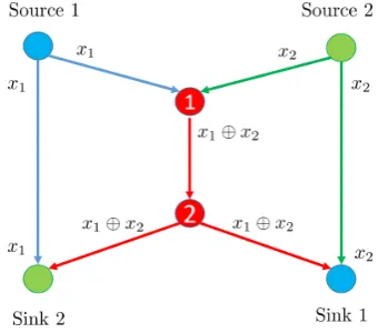
For instance consider the network topology below. Two sources wish to send 1 bit of data (x1 and x2) to their respective sinks through wired links, all having a capacity of 1 bit per transmission. In this instance, intermediate Node 1 is the bottleneck node, as it has to first forwardx1 and thenx2, which incurs extra waiting time to Sink 2. We also note that, although there are direct links between Source 1 and Sink 2 and between Source 2 and Sink 1, these links are not helpful.

1.1. A Brief History of Network Coding

To alleviate the tension, certain congestion control methods can be applied to different parts of the network. On one hand, the source may reduce its trans-mission rate upon congestion. For example, transtrans-mission control protocol (TCP) of the source may halve its transmission rate, or even back-off if congestion per-sists [1]. On the other hand, intermediate nodes may prioritize the incoming flows for better quality of service (QoS) [2]. Typical metrics include data type (e.g., assign higher priority to video streaming and lower priority to file downloading) and price (e.g., assign higher priority to the flows for subscribed users).

However, congestion control is not the optimal solution because it is not able to increase the overall network throughput, but may even reduce it sometimes. It was a common assumption that it is hardly possible to improve network through-put without infrastructure upgrade, until the invention of network coding (NC). The year of 2000 witnessed the official birth of NC. In their ground-breaking paper [3], Ahlswede et al. proposed that intermediate nodes do not just forward data flows but mix them together using certain coding techniques, which is now widely known as network coding. Based on the idea of NC, the function of Node 1 in Fig. 1.1 can be modified to that in Fig. 1.2: instead of forwardingx1 and then x2, Node 1 now generates a binary XOR of the two bits, i.e., x1⊕x2, which is still 1 bit. This NC bit is then sent to both sinks using one transmission. Since Sink 1 and Sink 2 have overheard x2 and x1 through the direct link from the other source, respectively, they can decode their wanted bit by solving a set of two simple linear equations. For example, for Sink 1 the equations are:

  

y1 =x2 y2 =x1 ⊕x2

where y1 and y2 represent the two bits it has received.

Ahlswede et al. then proved the optimality of NC by showing that it can achieve the min-cut-max-flow capacity [3] of wired multicast. Explicitly, they showed that NC allows every demanding sink to receive information from the source at the maximum rate, which is equal to the minimum sum capacity of the sets of links that cut off this sink from the source. However, they did not specify how NC should be implemented to optimally achieve the network capacity region, which is a core NC problem.

The optimal NC for wired multicast remained unclear until Liet al. proposed the concept of linear network coding (LNC) [4] in 2003. In LNC, the data unit is a vector over a certain finite field Fq, and is called a message or, in practical

Figure 1.2: Network coding breaks the capacity bottleneck of the butterfly net-work.

from Fq to generate NC packets for transmissions. Li et al. proved that LNC

suffices to achieve the min-cut-max-flow capacity of wired multicast. This result was confirmed again by Koetteret al. through proposing an algebraic framework of network coding [5].

The next milestone in the NC literature is the invention of random linear net-work coding (RLNC) [6] by Ho et al. in 2005, for it enables optimal, robust, yet fully decentralized implementations of NC. In RLNC, each node simply generates random linear combinations of all incoming packets using randomly picked coef-ficients from Fq. It was proved that RLNC is asymptotically capacity-achieving

in wired multicast when the size of Fq is sufficiently large [6].

For other networks where the connections are not multicast, it has been proved in [5] that their capacity optimization using NC is generally an NP-complete problem1_{. It has also been shown by Dougherty et al. in [8] that for certain} non-multicast networks, the NC capacity achieved by linear NC is strictly less than non-linear NC.

For the general NC optimization problem in arbitrary networks, useful math-ematical equivalences have been found. It has been shown by Dougherty et al. in [9] that the NC problem is closely related to matroid theory, a branch of ab-stract mathematics that studies the independence of elements [10]. It has been proved by Rouayheb et al. in [11] that both the NC problem and the

represen-1_{NP stands for “non-deterministic polynomial time”. An NP-complete problem cannot be}

1.2. Wireless Network Coding: New Challenges

tation problem of matroids can be reduced to an index coding (IC) problem. In IC, there is a single source and multiple sinks that are directly connected to the source. Every sink has already received a subset of the messages held by the source as its side information [11–15], and still wants one [11–14] or some [15] of the remaining messages. We will revisit IC in Section 1.4.4.

Although a sound theoretical basis has been established for NC in wired net-works, it could be difficult to integrate NC into existing wired networks such as the Internet. The main reason is that NC requires special network topologies that enable overhearing: as was explained in previous examples, in order to decode the received NC packet from a link, a sink must overhear some side information from other link(s). The side information could be combinations of data pack-ets it wants (intra-session NC) and/or combinations of data packpack-ets it does not want (inter-session NC) [16]. The other reason is that every intermediate node, especially the bottleneck node, must be able to perform NC, which may require hardware and protocol upgrades.

Whilst wired networks’ inherent features hinder the implementation of NC, there is another class of networks that intrinsically enables side information and does not impose the existence of intermediate nodes, namely, wireless networks. In the next section, we will review wireless NC.

1.2

Wireless Network Coding: New Challenges

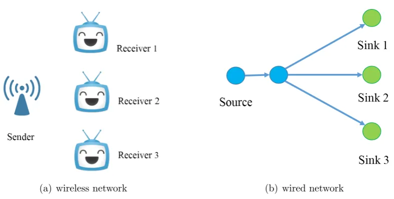
A basic wireless network consists of a sender and a set of wireless receivers within the transmission range of the sender. Due to the broadcast nature of the wireless media, every transmitted packet from the sender can be heard by every receiver. To fully exploit this feature, in this thesis we will use wireless networks for broad-cast, a scenario where every receiver wants all the data packets held by the sender. We note that broadcast is a subset of multicast.

From a network topology point of view, a wireless network is equivalent to a wired network where the source is connected to an intermediate node, and this node is connected to every sink through a different link (for example see Fig. 1.3). Hence, all the NC theorems and implementations developed for wired networks should be readily applicable to wireless networks. For example, it is straightforward that LNC suffices to achieve the optimal capacity of wireless multicast and broadcast.

(a) wireless network (b) wired network

Figure 1.3: A basic wireless network and its wired equivalence.

their wired counterpart. The most noticeable one is that wireless channels are much more lossy than wired links [17]: packets sent through wireless channels may be erased due to fading and interference and other imperfect channel conditions, which is much less likely to happen in wired links and can be efficiently treated with error correction codes therein. To compensate for packet losses in wireless networks, packet retransmissions are needed.

Consequently, a typical problem setting in wireless broadcast is that each receiver has only received a subset of a block of data packets, and still wants all the remaining data packets. Efficiently recovering these missing data packets is the design goal of coding techniques, and calls for the solving of several challenges. A core challenge is to minimize the number of retransmissions. This is because the number of retransmissions is inversely related to the system throughput, which is measured by the average number of packets delivered per transmission, and is a common alternative optimization goal to network capacity in practical wireless systems.

Another challenge is to minimize feedback cost. Due to the presence of packet erasures, receiver feedback must be collected for reliable data delivery [18, 19].2 For example, each receiver should at least send one Acknowledgement (ACK) notification upon reception of all wanted packets from the current block. Oth-erwise, the sender cannot decide when to stop sending the current block. How-ever, it could be expensive to collect feedback in wireless networks due to the

2_{There are also feedback-free techniques such as forward-error-control codes. But they have}

1.2. Wireless Network Coding: New Challenges

bandwidth limitation of the uplink and the energy limitation of the receivers. One such example is wireless sensor networks, where receivers are remote sensors with very limited energy and access to the network. Therefore, the amount of feedback should be minimized in practical implementations of wireless NC tech-niques [18–21, 21–24].

Besides throughput and feedback, the exploding demand for wireless video streaming raises an important challenge that has been largely overlooked in wired NC techniques, namely, minimizing average packet decoding delay (APDD). NC packets must be decoded before being usable, which only happens after the recep-tion of a certain number of NC packets. This incurs decoding delay of individual data packets [18, 25]. A large APDD is acceptable for applications where data packets are only useful as a whole (e.g., file downloading), but is undesirable or even unacceptable when individual data packets are useful or have a hard deadline (e.g. multi-layer image transmission and video streaming [26–28]).

Moreover, since wireless devices usually have limited energy and hardware resources, the computational complexity of applying NC is a non-negligible aspect in designing wireless NC techniques [29,30]. Some major sources of computational complexity are the complexity of making coding decisions and the complexity of performing the encoding and decoding.

In summary, optimizing throughput, APDD, feedback, and computational complexity are the main challenges in the design of NC techniques for wireless broadcast. Among them, throughput and APDD are the main performance met-rics, whilst feedback and computational complexity are implementation costs. In particular, the challenge of optimizing throughput can be solved by LNC.

Therefore, the main theme of this thesis is a comprehensive study on the throughput and APDD optimization for wireless broadcast using LNC. Imple-mentation costs will also be considered and minimized whenever applicable. Fol-lowing this theme, in this thesis we will present a four-part study. In the rest of this introduction, we will first outline the scope and structure of the thesis. We will then review the literature, and then summarize our contributions.

Before moving on, we remark, as a side note without diving into the details, that studying wireless NC can motivate the design of over-the-top (OTT) NC solutions for wired networks [31]. In such solutions, NC is only applied at the servers and sinks, and the underlying network is treated as a wireless-like media and unaltered. Examples of commercialized products are mainly peer-to-peer (P2P) based, such as Microsoftr _{Avalanche for its content distribution (e.g.,}

Figure 1.4: Thesis structure.

1.3

Thesis Scope and Structure

The fundamental problem addressed in this thesis is:

Problem 1.1

What is the achievable throughput and APDD performance of LNC in wireless broadcast and how to achieve them?

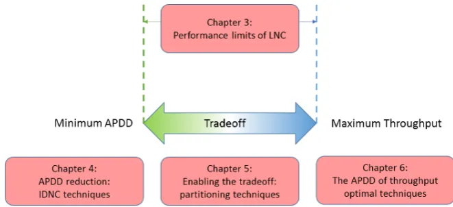
In order to comprehensively solve this problem, we will study LNC’s spectrum in terms of throughput and APDD performance, which includes the individual limits of the two, as well as their tradeoff. To this end, we will formally model the wireless broadcast system in Chapter 2, and then conduct a four-part study. The thesis structure is sketched in Fig. 1.4, and is elaborated as follows:

• Chapter 3 studies the throughput and APDD performance limits of LNC, as well as the hardness to find the optimal strategies to achieve such limits.

Our approach is to study LNC in its abstract form using mathematical theories such as matroid theory (a branch of mathematics that captures and generalizes linear independence in vector space [10]) and hypergraph theory. No specific LNC techniques will be studied. Therefore, results obtained from this chapter apply to all LNC techniques;

• Chapter 4 studies a class of LNC techniques that aim at reducing APDD.

1.4. Network Coding for Wireless Broadcast: A Review

• Chapter 5 studies the achievable tradeoff between throughput and APDD.

By partitioning a large set of data packets into smaller ones before applying LNC, it is possible to tune the tradeoff between throughput and APDD. Such techniques are well-known as generation-based LNC techniques. We will establish and study the optimal partitioning problem, develop its im-plementations, and evaluate its performance.

• Chapter 6 studies the APDD of throughput-optimal LNC techniques.

In order to obtain general results, we will apply an abstract model of such LNC techniques rather than specific ones. We will then develop a new throughput-optimal LNC techniques that aims at minimizing APDD, and compare its performance with existing ones, such as the classic random linear network coding (RLNC).

We will then conclude the thesis in Chapter 7.

In summary, we have briefly outlined the theme of each chapter. To provide deeper insights and to stress the contribution of this thesis, in the next section we will review the current art of the aforementioned classes of LNC techniques, as well as elaborate the knowledge gaps. Closing these gaps will be the main focus of the corresponding chapter.

1.4

Network Coding for Wireless Broadcast: A

Review

To motivate the development of NC techniques for wireless broadcast, we first briefly discuss a classic uncoded wireless retransmission technique called Automatic-Repeat-reQuest (ARQ). When ARQ is applied, the sender retransmits in each transmission the data packet requested by the most receivers [19].

1.4.1

Throughput-optimal Linear Network Coding

The iconic technique in this class is RLNC. Every RLNC packet is a random linear combination of all data packets in a block. For a receiver who is missing w data packets out of a block of K data packets and has received the rest, RLNC allows this receiver to decode all its w missing data packets w.h.p. (with high probability) upon the reception of any w RLNC packets. Hence, if this receiver does want all its wmissing data packets, which is the case in wireless broadcast, then every RLNC packet is useful to it w.h.p. until it has decoded these w packets. Consequently, RLNC is asymptotically throughput-optimal in wireless broadcast.

RLNC also minimizes the amount of receiver feedback. Due to randomized encoding, the sender does not need receivers’ packet reception state to make cod-ing decisions. It only requires one block completion ACK from each receiver, and will stop broadcasting the current block when all receivers have acknowledged.

However, RLNC has two drawbacks. The first one is a large APDD. Generally speaking, none of the wantedwdata packets can be decoded out until the receiver has received at leastwRLNC coded packets and has completed a block decoding procedure. Consequently, every data packet experiences a decoding delay of at leastw. The other drawback is a high computational complexity: O(w3_{) to solve} a set ofwlinear equations. The complexity will be further increased when a large finite field size is applied to increase the successful decoding probability.

Various efforts have been made to reduce the computational complexity of RLNC. It has been suggested in [29] that a systematic phase is applied before RLNC, where all data packets are broadcast uncoded once. [29] also suggested binary coding to further reduce the computational complexity at the cost of a graceful degradation in throughput. RLNC with random sparse coefficients (namely, coefficients are more likely to be zeros) [35–38] have been proposed to substantially reduce the computational complexity with graceful degradation on the throughput. There are also throughput-optimal techniques with sparse deterministic coefficients [39], which generate coded packets by collecting receiver feedback after every transmission and solving a hitting-set problem.

1.4. Network Coding for Wireless Broadcast: A Review

much design flexibility for APDD minimization.

To address the above two drawbacks of RLNC, another class of LNC tech-niques was invented to enable instant packet decodings under the binary field, which we now review.

1.4.2

Instantly Decodable Network Coding (IDNC)

Instant packet decodings refer to the case where a receiver instantly decodes a data packet upon the reception of one NC packet. For example, in Fig. 1.2, Sink 1 (resp. Sink 2) can instantly decode x1 (resp. x2) upon the reception of x1⊕x2 if it already has x2 (resp. x1).

LNC techniques that aim at providing such packet decodings are called in-stantly decodable network coding (IDNC) [21, 26, 27, 40–46]. The idea is to send in each transmission the binary XOR of a selected subset of data packets. Since both coding and decoding are operated under the binary field, IDNC techniques are also computationally friendly. Hence, IDNC techniques are very attractive in delay-sensitive applications where the receivers have limited computational resources, such as video streaming to mobile receivers [26, 27].

The main limitation of IDNC is a generally sub-optimal throughput perfor-mance because an instantly decodable packet to a subset of receivers may be useless to some other receivers. It has been shown that IDNC is asymptotically throughput-optimal if there are at most three receivers or the block size is in-finite [26]. But the exact characterization of the throughput of IDNC with a larger number of receivers is unknown in the literature. The other limitation is its dependence on receiver feedback to make coding decisions.

Besides receiving instantly decodable or useless packets, a subset of receivers may receive non-instantly decodable packets. For example, if in Fig. 1.2 there is a Sink 3 that has not received any bit, then Sink 3 will find x1⊕x2 useful (in the sense that it contains new bits that Sink 3 does not know) but not instantly decodable. IDNC techniques that prohibit the transmission of non-instantly de-codable packets are called strict IDNC (S-IDNC) [40, 43], whilst those allow such packets are called general IDNC (G-IDNC) [26, 27, 41, 42]. S-IDNC transmissions can thus be thought of as a subset of G-IDNC transmissions.

requires solving an NP-hard graph coloring problem [43], and the optimal value does not have a closed-form expression yet. Besides, there has not been any optimization results on the APDD of S-IDNC. Similarly, the best throughput and APDD of G-IDNC are unknown, too.

In summary, IDNC techniques trade throughput off for lower APDD by en-coding only a subset of data packets, whilst RLNC trades APDD off for optimal throughput by encoding all data packets together. There is another class of LNC techniques that somewhat sits between RLNC and IDNC: in this class, RLNC is applied to different subsets of data packets from the current block separately. We refer to this class as generation-based LNC techniques and will review it next for its potential in APDD reduction and achieving a better throughput-delay tradeoff.

1.4.3

Generation-based Linear Network Coding

Generation-based LNC techniques [48–53] were first introduced to reduce the decoding computational complexity of RLNC. The idea is to partition a block of data packets into small generations, and then apply RLNC to these generations separately. Consequently, each generation requires solving a smaller set of linear equations than applying RLNC without partitioning. Decoding computational complexity is thus reduced at the cost of a graceful degradation in throughput.

This class may also reduce APDD because data packets are now decoded per generation rather than per whole block [53]. By tuning the generation size, it is even possible to tune the throughput and APDD performance. However, most of the existing results on this class do not provide much insight on APDD minimiza-tion, partly because this is not their application focus, and partly because they do not collect receiver feedback for partitioning. Hence, studying and optimizing the APDD of feedback-assisted generation-based LNC is a new research topic.

1.4.4

Related Coding Techniques

1.5. Contributions

Index Coding

With proper reduction, the throughput optimization problem of LNC in wireless broadcast can be reduced to a very well studied retransmission minimization problem of IC [11–14]. The approach is to split every receiver that wants multiple data packets in wireless broadcast to multiple (virtual) receivers that only want one data packet in IC.

However, APDD minimization has not been considered in the IC literature. Moreover, most works in the IC literature assume no packet erasures, which is generally not the case in wireless broadcast. Therefore, the problems we will solve in this thesis are different from those in the IC literature, and may provide new insights into the problems in the IC context.

Fountain Codes

Fountain codes (FC) [54–56] are also asymptotically throughput-optimal codes that can work equally well in wireless broadcast as RLNC. With appropriate pre-coding of the input data packets, FC are able to offer linear time encod-ing and decodencod-ing complexity per data packet. However, FC are not necessarily throughput-optimal in more complex networks with relays, because the relays have to decode and re-encode. Moreover, FC in general do not offer as much flexibility in the design and ease of implementation as NC, e.g., when APDD is to be minimized.

According to the above literature review, it is clear that APDD minimization has been largely overlooked in the literature. There has not been a comprehensive study on it, nor any optimization or approximation techniques3 _{for it. Moreover,} the interplay between APDD, throughput, feedback, and computational complex-ity has not been well understood in wireless broadcast. These gaps motivated this thesis. In the next section, we will summary the contributions of this thesis.

1.5

Contributions

In this thesis, we will solve Problem 1.1 and close the aforementioned knowledge gaps by applying a wide range of mathematics theories such as matroid theory, graph theory, hypergraph theory, finite field theory, and stochastic processes. Our main contributions are as follows:

3_{A technique is aβ-approximation technique of APDD if its APDD performance is at most}

1. [Chapter 3] We deduce a necessary and sufficient condition for LNC to achieve the optimal throughout of wireless broadcast under any given Fq;

2. [Chapter 3]We prove the NP-hardness of using LNC for APDD minimiza-tion;

3. [Chapter 3] We derive closed-form lower bounds of the expected APDD of LNC in wireless broadcast;

4. [Chapter 4] We prove that S-IDNC is not able to approximate the min-imum APDD in general. But it is able to optimize both throughput and APDD when there are at most three receivers. We develop optimal and heuristic S-IDNC algorithms.

5. [Chapter 5] We establish the optimal partitioning problem and prove its NP-hardness. We develop a heuristic partitioning algorithm that achieves local Pareto-optimal4 _{throughput-delay tradeoff;}

6. [Chapter 6] We prove that all throughput-optimal LNC techniques are APDD-approximation techniques with a ratio of between 4/3 and 2. In particular, the approximation ratio of RLNC is exactly 2;

7. [Chapter 6]We develop a throughput-optimal and APDD-approximation LNC technique that: 1) always provides instant packet decodings; 2) has an approximation ratio of strictly smaller than 2; 3) uses a polynomial-time encoding algorithm; and 4) does not require intensive receiver feedback.

We also conduct extensive simulations to verify the proposed theorems and properties, and to demonstrate the superiority of the new techniques over existing ones. Most of the results of this thesis have been presented in academic papers, including 7 published ones and 1 under preparation:

1. M. Yu, N. Aboutorab, P. Sadeghi,“From instantly decodable to random linear network coded broadcast,” IEEE Trans. Comm., vol. 62, no. 11, pp. 3943–3955, 2014.

2. M. Yu, P. Sadeghi, N. Aboutorab,“Performance characterization and trans-mission schemes for instantly decodable network coding in wireless broad-cast,” Euro J. Advances in Signal Processing, vol. 94, 2015.

4_{A tradeoff between two metrics is Pareto-optimal if neither metric can be improved without}

1.5. Contributions

3. M. Yu, P. Sadeghi, A. Sprintson,“The benefit of limited feedback to generation-based random linear network coding in wireless broadcast,” inProc. IEEE Global Communications Conference (GLOBECOM) Workshop , 2016. 4. M. Yu, A. Sprintson, P. Sadeghi, “On minimizing the average packet

decod-ing delay in wireless network coded broadcast,” in Proc. IEEE Int. symp. Network Coding (NetCod), 2015.

5. M. Yu, P. Sadeghi, N. Aboutorab,“On deterministic linear network coded broadcast and its relation to matroid theory,” in Proc. IEEE Information Theory Workshop (ITW), 2014.

6. P. Sadeghi, M. Yu, N. Aboutorab,“On throughput-delay tradeoff of network coding for wireless communications,” (invited paper) in Proc. IEEE Int. Symp. Information Theory and its Applications (ISITA), 2014.

7. M. Yu, N. Aboutorab, P. Sadeghi,“Rapprochement between instantly de-codable and random linear network coding,” in Proc. IEEE Int. Symp. Information Theory (ISIT), 2013.

Chapter

2

Modeling Linear Network Coded

Wireless Broadcast

In this chapter, we review how linear network coding (LNC) can be applied in wireless broadcast systems for performance improvements. We will introduce the basic system settings, demonstrate the general implementation of LNC, define the performance measures, and briefly introduce two LNC techniques that aim to optimize these measures.

2.1

System Model

2.1.1

Basic Settings

We consider a wireless broadcast system depicted in Fig. 2.1. It involves one sender and a set of N receivers, denoted by _R = _{rn}Nn=1. The sender holds a block ofK data packets, denoted by _P =_{pk}Kk=1, and wishes to deliver them to all receivers. All data packets are modelled as equal-length vectors over a given finite field Fq, where q is a power of a prime. In the simplest setting, q is equal

to 2 and all data packets are sequences of binary bits.

Time is slotted. In each time slot, the sender broadcasts a packet to all receivers. Due to imperfect wireless media, each receiver rn either misses the

packet with a probability of Pe,n, or correctly receives it with a probability of

1−Pe,n. In other words, the wireless downlink from the sender to each receiver

rn is subject to independent and Bernoulli distributed packet erasures with an

erasure probability ofPe,n. This is a common model for wireless erasure broadcast

2.1. System Model

We can think of the K data packets as the K orthogonal bases of a K -dimensional knowledge space. A receiver is able to retrieve these K bases iff it can reproduce this space. To this end, it will need a set ofK linearly independent vectors of this space, where each vector is either a basis or a linear combination of the bases. In LNC context, such a combination is called aNC coded packet. It is denoted by X and takes a form of:

X = X p∈M

αkpk (2.1)

where _{αk} are non-zero coding coefficients chosen from Fq, and M ⊆ P is the

set of data packets with non-zero coding coefficients. We call _M the coding set of X and call X a coded packet of _M. At a high level, every LNC technique is a method of choosing _M and _{αk}. Upon the reception of sufficient data and

coded packets, the K-dimensional knowledge space can be reproduced, and thus all the K bases can be retrieved through solving linear equation(s).

2.1.2

Transmission Phases

Optimally choosing _M and _{αk} is trivial in the initial phase of the broadcast.

The sender can simply broadcast every data packet uncoded once using K time slots. This phase is called thesystematic transmission phase. In this phase, every packet transmission is innovative to every receiver, where:

Definition 2.1

A (data or coded) packet is innovative to a receiver rn if it allows rn to

increase the dimension of its knowledge space by one. In other words, this packet is linearly independent of the set of packets that rn already has.

Therefore, every transmission in this phase isthroughput-optimal, where:

Definition 2.2

The transmission of a (data or coded) packet is throughput-optimal if the packet is innovative to every receiver who is still missing packets.

Sender

r1 Pe,1

r2 Pe,2

rN

Pe,N

...

p1 p2 _{· · ·} pK

Figure 2.1: The wireless broadcast ofK data packets to N receivers.

p

p

p

r

1

0

0

r

0

0

1

r

0

1

0

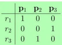
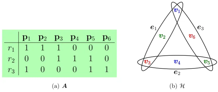
Figure 2.2: An example of state feedback matrix A

and A(n, k) = 0 meansrn already has pk. The set of data packets wanted byrn

is called the Wants set of rn and is denoted by ωn. The size ofωn is denoted by

wn. The set of ωn of all receivers is denoted byW. The set of receivers who want

pk is called the Target set of pk and is denoted by τk. The size of τk is denoted

by tk. An example of SFM is demonstrated in Fig. 2.2, in which ω1 ={p1} and τ2 ={r3}.

2.1. System Model

Example 2.1

Consider the SFM in Fig. 2.2. Receiver r1, r2, and r3 only want p1, p3, andp2, respectively, and have received all the remaining data packets. Re-transmitting{p1,p2,p3} separately will cost 3 transmissions, but a coded packet of X = p1 ⊕p2 ⊕p3, where ⊕ is the binary XOR operator, will allow all receivers to decode their missing data packets upon the reception of X. For example, r1 can decode p1, as p1 =X ⊕p2⊕p3.

Hence, after the systematic transmission phase, the sender applies an LNC technique and transmits coded packets until the broadcast is complete, i.e., until all receivers have retrieved all the K data packets. These coded transmissions constitute the second phase of the broadcast, called thecoded transmission phase. In the next chapter, we will study the achievability of throughput-optimality in this phase.

2.1.3

Classes of Linear Network Coding Techniques

To generate the coded packet in each coded transmission, the sender needs to select the coding set M and the coding coefficients {αk}. The way they are

selected broadly classifies LNC techniques into two types:

• Random techniques, in whichMis randomly selected from P, and/or{αk}

are randomly selected from Fq;

• Deterministic techniques, in which M and/or {αk} are deterministically

selected (from Fq for{αk}).

For example, the RLNC technique sets M = P, and chooses {αk}Kk=1 uni-formly at random fromFq. For another example, the instantly decodable network

coding (IDNC) technique strategically choosesM, and then adds all data packets inMtogether under the binary field F2. We will discuss these two techniques in more detail by the end of this section.

2.1.4

Receiver Feedback

after this receiver has retrieved all data packets. Upon the reception of this feedback from all receivers, the sender can complete the broadcast of the cur-rent block. Besides, deterministic LNC techniques require one round of feedback immediately after the systematic transmission phase to construct the SFM. In ad-dition, the sender may also collect feedback during the coded transmission phase. The explicit feedback frequency of different LNC techniques will be discussed in later chapters.

In summary, we consider a two-phase wireless broadcast of K data packets to N receivers through wireless channels that are subject to independent packet erasures. In the systematic transmission phase, data packets are transmitted uncoded once. Then in the coded transmission phase, coded packets are trans-mitted, where each is a linear combination of the data packets generated using an LNC technique. Receivers send feedback at an appropriate frequency (depending on the LNC technique) to assist the sender in making coding decisions. They solve linear equation(s) to retrieve all data packets.

As demonstrated in Example 2.1, applying LNC after the systematic transmis-sion phase can significantly improve the broadcast efficiency compared with un-coded packet retransmission schemes, such as Automatic-Repeat-reQuest (ARQ) [19]. In this thesis, we consider two fundamental performance measures, namely, throughput and packet decoding delay, which are defined next.

2.2

Throughput and Decoding Delay Measures

In this section, we define the throughput and packet decoding delay measures. For each measure we will introduce an LNC technique that aims to optimize it.

2.2.1

Throughput and RLNC

We denote byUthe total number of transmissions in the coded transmission phase in the broadcast of a block of K data packets, and call it the block completion time (BCT). U is inversely related to throughput, because the system spends a total of K +U transmissions to broadcast a set of K data packets, yielding a throughput of K

K+U packet per transmission. Hence, maximizing throughput is

equivalent to minimizing U.

2.2. Throughput and Decoding Delay Measures

Definition 2.3

For a receiverrnwithureceived coded packets, its coding coefficient matrix

Cn is an u×K matrix under Fq, where Cn(i, k) is the coefficient of pk in

the i-th coded packet:

Cn =

     

α1,1 α1,2 · · · α1,K

α2,1 α2,2 · · · α2,K

... . .. ... ... αu,1 αu,2 · · · αu,K

     

u×K

(2.2)

We can then easily prove the following decoding condition:

Condition 2.1

In order to allowrnto decode all the data packets inωn, the set of columns

of Cn indexed by ωn must have a rank of wn.

For example, if rn wants ωn = {p1,p2,p3}, then the first three columns of

Cn must have a rank of 3, so that rn can decode {p1,p2,p3} through solving a

set of 3 linear equations.

To satisfy this condition, the number of received coded packets must satisfy u > wn, because otherwise with u < wn rows, the rank of the columns can at

most be u, but never be wn. The minimum value of u is wn and is achieved iff

every received coded packet is innovative (defined in Definition Definition 2.1) to rn.

Therefore, the BCT U is minimized when every receiver rn can decode all

its wn wanted data packets after receiving wn coded packets. This requires that

every transmitted coded packet must be innovative to every receiver who is still missing packets. Consequently, we have the concept of throughput-optimal LNC technique:

Definition 2.4

A LNC technique is throughput-optimal if the transmission of every coded packet generated by it is throughput-optimal.

There-fore, Cn is a matrix with randomly valued entries. When Fq is sufficiently large,

RLNC asymptotically ensures that any wn×wn sub-matrix of Cn has a rank of

wn. Therefore, upon the reception of anywnRLNC coded packets, every receiver

rn can decode its wn wanted data packets by solving a set of wn linear equations

provided by these wn RLNC coded packets.

Due to its random nature of coding, RLNC has an additional advantage that it does not require intermediate feedback after the systematic transmission phase and during the coded transmission phase. But there are two main problems in using RLNC. The first one is high decoding computational load:

Definition 2.5

Each receiver performs Gaussian eliminations to solve linear equations. The computational load of solving a set of w linear equations is _O(w3₎ opera-tions.

We can then easily show that the maximum computational load of a receiver rn is O(wn3). This maximum is reached by RLNC because rn has to solve a set

of wn linear equations in the RLNC decoding process. Hence, RLNC requires

the highest decoding computational load among all LNC techniques. The above decoding process also implies the second and main problem of RLNC, namely, RLNC is inefficient in terms of packet decoding delay, which we now define.

2.2.2

Average Packet Decoding Delay (APDD) and IDNC

When LNC is applied, it is likely to be the case that a receiver has to collect a certain number of coded packets before being able to decode any individual data packet. This feature is acceptable if the receivers are only interested in the block of data packets as a whole. But this is undesirable in applications where individual data packets are useful, such as image transmissions and video streaming [26, 28, 57]. Therefore, we are interested in the decoding delay of the individual data packets. We measure this performance through the average packet decoding delay (APDD), denoted by D:

D= 1 T

X

∀n,k:An,k=1

un,k (2.3)

where un,k is the index of the coded transmission when rn decodes pk, and T =

PK

2.2. Throughput and Decoding Delay Measures

the number of “1”s in A. Note that in this thesis we do not consider ordered packets. Thus, all the data packets have the same decoding priority.

We note that D is the overall APDD of A under a realization of the coded transmission phase. Applying the same idea, we can also calculate the APDD experienced by each receiver rn, denoted byDn:

Dn =

1 wn

X

∀k:pk∈ωn

un,k (2.4)

We further note that there are also other measures of packet decoding delay in the literature. A common one is that a receiver experiences one unit increase of decoding delay if it has received a coded packet, but cannot decode any new data packet from it [58]. However, this measure does not consider the exact decoding delay of each data packet, and thus cannot fully reflect the packet decoding delay performance of LNC techniques. To see this, consider the following example:

Example 2.2

Consider two receivers: r1 decodes one wanted data packet in the first and third coded transmissions, respectively, but cannot decode in the second coded transmission; r2 decodes one wanted data packet in the second and third coded transmissions, respectively, but cannot decode in the first coded transmission. According to the above measure, the packet decoding delay experienced by bothr1 andr2 is 1. However, it is obvious thatr1 has faster packet decodings. If our measure is applied, the APDD of r1 and r2 is 2 and 2.5, respectively.

It is intuitive that the key to reducing D is to reduce the number of coded packets that each receiverrn needs to collect before being able to decode

individ-ual data packets. In the best case scenario,rncaninstantly decode a wanted data

packet using only one coded packet. To this end, the coding set of this coded packet must contain only one wanted data packet ofrn, i.e.,|M∩ωn|= 1. A

well-known class of deterministic LNC techniques that aim at designing such coded packets is called IDNC. The coded packet we have generated in Example 2.1 is an IDNC coded packet.

are not necessarily throughput-optimal because there may exist a subset of re-ceivers with their |ωn∩ M| = 0, who will find the corresponding coded packet

non-innovative.

2.3

Conclusion

In this chapter we have established the network coded wireless broadcast system considered in this thesis. We have also introduced the main performance measures that will be optimized in this thesis, including block completion time U and average packet decoding delay D. We have also shed some light on how could they be reduced by using specific LNC techniques such as RLNC and IDNC.

Chapter

3

Fundamental Limits of Linear

Network Coded Wireless Broadcast

This chapter focuses on the fundamental performance limits of linear network coding (LNC) in wireless broadcast. The two performance measures are the block completion timeU and the average packet decoding delayDdefined in the last chapter. AlthoughU andDvary under different LNC techniques, there exist lower bounds ofU and Dthat no LNC technique can break. Studying the values and achievability of these bounds is important for understanding the fundamental limits of LNC.

To this end, we will first study the lower bounds of U and D for any given state feedback matrix (SFM) by assuming no packet erasures in the coded trans-mission phase. The results will also serve as fundamental limits in the presence of random packet erasures. Then by further assuming random packet erasures, we will derive lower bounds of the expectedD, and study its relation with system parameters, including the number of data packets and receivers and the packet erasure probability. We will not study the expectedU, as this is well understood in the literature, e.g., by studying the distribution of U of RLNC [59] under random packet erasures, as RLNC is able to asymptotically minimizesU.

3.1

Throughput

Given a SFM A, we denoted by Umin the minimum possible block completion

time (BCT) that LNC techniques can achieve. The value of Umin is

3.1. Throughput

needs at least wn coded packets to decode its wn wanted data packets.

We then study the achievability ofUmin under a finite fieldFq by considering

the coefficient matrix of a set of Umin coded packets:

C =      

α1,1 α1,2 · · · α1,K

α2,1 α2,2 · · · α2,K

... . .. . .. ... αUmin,1 αUmin,2 · · · αUmin,K

     

Umin×K

(3.1)

According to the decoding condition defined in Condition 2.1 in the last chap-ter, a receiverrncan only decode all its wanted data packets fromCif the columns

ofCindexed byωnare linearly independent, for alln∈[1, N]. Hence, the

achiev-ability of Umin is translated into the existence of some C under Fq such that its

columns satisfy some linear independence constraints imposed by _W ,{ωn}Nn=1. This problem is closely related to a field in abstract mathematics called matroid theory [60], which has been extensively used to characterize the broader index coding problem. We will first briefly introduce matroid theory, and then develop its connection with our problem, which is the main contribution of this section.

3.1.1

Preliminaries of Matroid Theory

A matroid M is an ordered pair (E,I). E is a finite set of elements called the ground set. I is a family of subsets of E calledindependent sets. An independent set is denoted by I and its rank is equal to its cardinality, i.e., r(I) =|I|, where r(·) is a rank function. A maximal independent set is called a basis. All bases of a matroid have the same size and rank. Their rank is also the rank of M, denoted byrM. On the other hand, all the subsets of E not in I are dependent sets. The

meaning of independence can be visualized through a representation of matroid called matrix matroid.

Definition 3.1

AnrM × |E| matrix C over Fq represents a matroid M(E,I) and is called

a matrix matroid if the columns of C indexed by any I ∈ I are linearly independent, and those not indexed by I are linearly dependent.

A matroid is q-representable if it has a matrix representationC over Fq.

1 0 1 0 1 0

C=

Figure 3.1: The matrix representation of a matroid with E = {1,2,3} and I =

{1,2,3,(1,2),(2,3)_}.

the 2×3 binary matrix C in Fig. 3.1(a), because column sets (1,2) and (2,3) are linearly independent sets according to _I, while (1,3) is a dependent set.

There is a special type of matroid called uniform matroid, denoted by _UrM

K .

It is a matroid that 1) hasK elements, 2) has a rank ofrM, and 3) every size-rM

subset of the elements is a basis.

3.1.2

Achievability of

U

v.s. Matroid Representability

Recall that Umin is achieved iff there exists aUmin×K matrix C under Fq such

that its columns indexed by anyωn ∈ W are linearly independent. Compare this

condition with the definition of matrix matroid, we reach the following theorem:

Theorem 3.1:

A sufficient condition for the achievability of Umin under Fq is that the

uniform matroid _UUmin

K is q-representable. This condition becomes also

necessary if _W contains all the bases of _UUmin

K .

Proof. This theorem holds because the _I of _UUmin

K contains all the 1 to

size-Umin subsets of the K elements. Since every receiver rn wants at most Umin out

of K data packets, we have ωn ∈ I for every n ∈ [1, N], indicating that the

decoding condition on C required by rn can be satisfied by the matrix matroid

of _UUmin

K . Moreover, if every set of Umin data packets are wanted by a different

receiver, then _W contains all the bases of _UUmin

K . In this case, the only C that

achieves Umin is the matrix matroid of U_KUmin.

Example 2. Uniform matroid _U42 has a ground setE ={1,2,3,4}and a rank of 2. Every one-element and two-element subset of E is an independent set. Con-sider an SFM with K = 4 data packets and N = 6 receivers. Each receiver wants a different pair of two data packets, and thus Umin = 2. Both the representability

of _U42 and the achievability ofUmin requires a 2×4 matrix C such that every two

3.1. Throughput

Table 3.1: UUmin

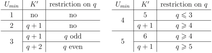
K is q-representable iff K 6K0.

Umin K0 restriction on q

1 no no

2 q+ 1 no

3 q+ 1 q odd

q+ 2 q even

Umin K0 restriction onq

4 5 q63

q+ 1 q>4

5 6 q>4

q+ 1 q>5

This requirement is not feasible under the binary field _F2, because there are only 3 distinctive length-2 non-zero columns under _F2 as shown below. Conse-quently, the 4-th column must repeat a previous column, which fails the require-ment. Hence, _U42 is not 2-representable and Umin cannot be achieved over F2.

On the other hand, _U42 is q-representable over any q > 3, and thus Umin can be

achieved as well.

C =

"

0 1 1 ? 1 0 1 ?

#

(3.2)

Theorem 3.1 indicates that the achievability of Umin under Fq can be

trans-lated into theq-representability of uniform matroidUUmin

K . However, this problem

is largely open: studies on the q-representability of UUmin

K is only complete for

Umin 6 5 [60], with results summarized in Table 3.1. For other values of Umin,

it is not clear under what Fq UKUmin is q-representable. Moreover, there has not

been a polynomial-time algorithm that optimally finds the matrix representation of a matroid [60].

Despite the openness of the problem, all existing results support a general conjecture that uniform matroids are more likely to be representable over large

Fq. For example, the well known maximum distance separation (MDS) conjecture

in coding theory argues, after some translation [61], that q>K −1.

Therefore, the achievability ofUminis an open problem in general and does not

have an optimal algorithm for its solutions. But Umin could be asymptotically

achieved over large Fq. For example, random linear network coding (RLNC)

chooses coding coefficients uniformly at random from a sufficiently large Fq, so

that in the Umin × K coefficient matrix of any Umin coded packets, any Umin

3.2

Average Packet Decoding Delay

Given a SFM A, we denoted by Dmin the minimum average packet decoding delay (APDD) that LNC can achieve even without packet erasures. Unlike Umin,

the value of Dmin has not been studied in the literature. In this section, we will prove that it is NP-hard to find and achieveDmin. We will then study the best D that LNC techniques can beexpected to achieve on average under random packet erasures.

For the proof of the NP-hardness of finding and achieving Dmin, our approach is to first derive a lower bound of Dmin, then prove the NP-hardness of achiev-ing this lower bound. This result will indicate the NP-hardness of findachiev-ing Dmin, because otherwise by findingDmin, we can immediately determine the achievabil-ity of the lower bound. The NP-hardness of finding Dmin will further indicate that it is NP-hard to achieve Dmin, because otherwise by achieving it, we can immediately find its value.

We start with presenting our newly developed lower bound on D, which can only be achieved by a perfect LNC solution.

3.2.1

The Perfect LNC Solution

A set of ordered coded packets{Xu}Uu=1 is called an LNC solution and is denoted by S if, upon the reception of all these coded packets, every receiver can decode all its wanted data packets. Then,

Definition 3.2

An LNC solution _S is called a perfect solution and is denoted by _Sp if it

al-lows every receiverrnto decode a wanted data packet in every transmission,

until rn has decoded all its wanted data packets.

According to its definition, Sp is throughput-optimal, for every transmission

is throughput-optimal. More importantly, Sp offers the ideal packet decodings.

Its average packet decoding delay (APDD), denoted by D0, is thus a lower bound onDmin, and is calculated as:

D0 = _PN1

n=1wn

N

X

n=1

wn

X

u=1

u (3.3)

=

PN

n=1w2n

2PN

n=1wn

+1

3.2. Average Packet Decoding Delay

p

p

p

p

p

p

r

1

1

1

0

0

0

r

0

0

1

1

1

0

r

1

0

0

0

1

1

v1

v2

v3 v4 v5

v6

v1

v2

v3 v4 v5

v6

e1

e2

e3

(b) _H

Figure 3.2: The hypergraph model_H of an SFM A

It is clear that D0 can only be achieved if Sp exists. The natural question in

this context is: Does a perfect solution _Sp exist for a given SFM A? In the next subsection, by using a reduction from the strong hypergraph coloring problem, we will prove that this question is NP-complete to answer.

3.2.2

The Hardness of APDD Minimization: A

Hyper-graph Coloring Approach

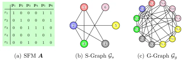
A hypergraph _H is defined by a pair (_V,_E), where _V is the set of vertices, and E is the set of hyperedges. Every hyperedge e _{∈ E} is a subset of _V with size |e_| > 1. _H can be used to model the packet reception instance. For each data packet pk we generate a vertex vk ∈ V, and for each receiver rn we generate a

hyperedge en ∈ E that is incident to the vertices/packets wanted by rn, i.e., let

en = ωn. An example of SFM and its hypergraph model are demonstrated in

Fig. 3.2. Similarly, given any hypergraph _H, we can also generate an SFM A. Hence, there is a bijection between Aand _H.

We then introduce some related concepts from the hypergraph theory. A hypergraph is r−uniform if the size of all hyperedges is r, i.e., |e| =r for every

e ∈ E. A size-k strong coloring of H is a partition of V into k subsets {Vi}ki=1, such that |Vi ∩e| 6 1 for every e ∈ E. In other words, if we assign k colors to

Lemma 3.1:

It is NP-complete to determine whether an r₋uniform hypergraph is size-r strong colorable or not, for any r>3.

This lemma indicates the hardness of finding Sp:

Corollary 3.1:

It is NP-complete to determine whether there exists a perfect solution for a given A.

Proof. Here we only need to prove that anr-uniform hypergraph is size-r strong colorable iff there exists a perfect LNC solution of the corresponding A, in which every receiver wants r data packets. If this is proved, then according to Lemma 3.1, it is NP-complete to determine the existence of a perfect solution for suchA. This will indicate that the problem is NP-complete under generalA.

First, we prove that a size-r strong coloring {Vi}ri=1 of H implies a perfect solutionSp of A. Since for every hyperedge it holds that|en|=r and there arer

colors, we have |Vi∩en|= 1. Let {Mi}ri=1 be the sets of packets corresponding to{Vi}ri=1. Then, we have|Mi∩ωn|= 1 for every receiver rn. Hence, the linear

sum of all data packets fromMi is a coded packet Xi that allows every receiver

to immediately decode a wanted data packet. Therefore, {Xi}ri=1 together form a perfect solution Sp of A.

Next, we prove that a perfect solutionSp of Aimplies a size-rstrong coloring

{Vi}ri=1 of H. Since every receiver wants r data packets, Sp contains r coded

packets {Xi}ri=1. In order to allow every receiver to decode one wanted data packet from Xi, the coding set Mi of Xi must contain exactly one wanted data

packet of every receiver, i.e., |Mi∩ωn| = 1. Let {Vi}ri=1 be the sets of vertices corresponding to {Mi}ri=1, it holds that |Vi∩en|= 1 for every hyperedge. Thus,

{Vi}ri=1 is a size-r strong coloring of H.

3.2. Average Packet Decoding Delay

Example 3.1

The SFM in Fig. 3.2(a) has a perfect solution that contains three coded packets: X1 =p1⊕p4, X2 =p2⊕p5, and X3 =p3⊕p6, where⊕ is the binary XOR operator. Then, by coloring {v1,v4}, {v2,v5}, and {v3,v6} in the corresponding hypergraphH using three different colors, we obtain a size-3 strong coloring ofH, as shown in Fig. 3.2(b).

SinceD0 can only be achieved by a perfect solution _Sp, an optimal algorithm

that finds Dmin will be able to determine the existence of a perfect solution through comparing Dmin with D0. According to Corollary 3.1, this decision is NP-complete to make, and thus it is NP-hard to find Dmin:

Theorem 3.2

It is NP-hard to find Dmin for a given SFM A.

This theorem also indicates that there is no network coding technique that can achieve Dmin using a deterministic polynomial-time coding algorithm unless P=NP.

3.2.3

APDD Approximation

Since Dmin is NP-hard to achieve, we are interested in its approximation. An LNC technique is said to be a β-approximation technique of Dmin if its APDD is at most β (inclusive) times ofDmin. Such a technique, upon its existence, will be highly appreciated for providing guaranteed APDD performance.

Definition 3.3

An LNC technique is said to be aβ-approximation technique of the APDD minimization problem if for any given SFM A and any packet erasure probability _{Pe,n}Nn=1 > 0, the expected APDD using this technique is at most β times of the minimum expected APDD of LNC.

Due to the NP-hardness of finding Dmin when {Pe,n}Nn=1 = 0, it is also NP-hard to find the minimum APDD of LNC under a more general setting on packet erasure probabilities. To solve this problem, in the next subsection we will derive lower bounds of the minimum expected APDD of LNC. These bounds will serve as the APDD performance limits of LNC under wireless broadcast, and will also help with verifying APDD-approximation techniques. This is because if a technique’s APDD is at most β times of the lower bound, then its approximation ratio is at most β.

3.2.4

Lower bounds of the Expected APDD

In this subsection, we derive lower bounds of the minimum expected APDD of all LNC techniques under random packet erasures. To this end, we will extend the concept of “perfect LNC solution” to “perfect LNC technique”, and study what APDD performance can be expected from this perfect technique under random packet erasures. The results will serve as lower bounds of the expected APDD of all LNC techniques. In particular, we are interested in two types of expectations:

• The expected APDD of a given SFM using LNC. The expectation will be the APDD averaged over all possible erasure patterns in the coded transmission phase;

• The overall expected APDD of the wireless broadcast system using LNC. The expectation will be the APDD averaged over all possible erasure pat-terns in both the systematic and coded transmission phases. The resultant expected APDD will reflect the overall APDD performance in terms of sys-tem parameters, including the number of data packets K, the number of receivers N, and the packet erasure probabilities {Pe,n}Nn=1.

3.2. Average Packet Decoding Delay

Definition 3.4

A perfect LNC technique allows every receiver to decode a wanted data packet whenever this receiver successfully receives a coded packet generated using this technique.

. Similar to the perfect LNC solution, a perfect LNC technique is also throughput-optimal, and also offers the ideal packet decodings.

In order to derive the expected APDD of all receivers when the perfect LNC technique is applied, we first derive the expected APDD of a single receiver. Let D_n denote the APDD of receiver rn under an arbitrary erasure pattern when

the perfect LNC technique is applied in the coded transmission phase. (Here the underline means lowed bound.) Then, by averaging over all possible erasure patterns, we obtain the expectedD_nofrn, which is given in the following theorem.

Lemma 3.2

When coded transmissions are subject to random packet erasures with a probability of Pe,n, the expected Dn of a receiver rn who wants wn data

packets is:

E[D_n|whenrn wants wn data packets] =

wn+ 1

2(1−Pe,n)

(3.5)

Its proof is given in Appendix B. In the rest of this subsection, we will simplify the notation for such conditional expectations to a form of E[a_|(b, c,_{· · ·})], which stands for the expectation of variable a when the values of variables b, c,_{· · ·} are given. For example, the expectation in (3.5) can be simplified to E[D_n|wn].

By applying this lemma, we can immediately obtain the following theorem:

Theorem 3.3

Let E[D|{wn}Nn=1] be the expected APDD of a given SFM A when the perfect LNC technique is applied, where {wn}N1 are known from A. Then,

E[D_|{wn}Nn=1] =

PN

n=1

w2

n+wn

2(1−Pe,n)

PN

n=1wn

(3.6)

This is a lower bound of the expected APDD ofA when LNC is applied.

APDD of each receiver:

E[D_|{wn}Nn=1] =

E[D₁|w1]·w1+E[D₂|w2]·w2+· · ·+E[D_N|wN]·wN

w1+w2+_{· · ·}+wN

=

PN

n=1

w2

n+wn

2(1−Pe,n)

PN

n=1wn

Since the perfect LNC technique minimizes the expected APDD of every receiver, it also minimizes the expected APDD of the SFM.

Then, by noting that the SFM Aitself is the consequence of random packet erasures in the systematic transmission phase, it is possible to derive the expec-tation of E[D_|{wn}Nn=1], i.e., E[E[D|{wn}Nn=1]], by averaging over all possibleA. The result is a more general lower bound:

Theorem 3.4

Given system parameters K,N, andPe, the overall APDD performance of

the perfect LNC technique is E[D], where

E[D] = 1 2(1−Pe)

1 +E

"_PN

n=1wn2

PN

n=1wn

#!

, _{wn}Nn=1 ∼B(K, Pe) (3.7)

≈ KPe−Pe+ 2 2−2Pe

, when N is sufficiently large (3.8)

This is a lower bound of the minimum expected APDD of LNC techniques.

Here (3.7) is obtained by letting {Pe,n} = Pe in (3.6) and taking the

expec-tation. Each wn follows a binomial distribution ofB(K, P e) because the packet

erasures follow a Bernoulli distribution defined byPe. We will prove in Appendix

E that Eh

PN n=1wn2

PN

n=1wn

i

≈KPe−Pe+ 1 when N is sufficiently large, which will prove

the estimation in (3.8).

According to (3.8), our proposed lower bound is independent of the number of receivers. This observation is confirmed by our simulations. The results for K = 15 data packets, N _∈ [5,100] receivers, and packet erasure probabilities of _{Pe,n}Nn=1 = 0.2 are shown in Fig. 3.3, which also affirm the accuracy of the proposed estimation.

We also note that, although the above theorem is derived by assuming a homogeneous packet erasure probability of {Pe,n}n1 =Pe, the result can be easily