Predicting Worst-Case Execution Time Trends in Long-Lived Real-Time Systems

This is a repository copy of

Predicting Worst-Case Execution Time Trends in Long-Lived

Real-Time Systems

.

White Rose Research Online URL for this paper:

http://eprints.whiterose.ac.uk/133478/

Version: Accepted Version

Proceedings Paper:

Dai, Xiaotian orcid.org/0000-0002-6669-5234 and Burns, Alan

orcid.org/0000-0001-5621-8816 (2017) Predicting Worst-Case Execution Time Trends in

Long-Lived Real-Time Systems. In: Bader, Markus and Blieberger, Johann, (eds.) Reliable

Software Technologies - Ada-Europe 2017 - 22nd Ada-Europe International Conference on

Reliable Software Technologies, Proceedings. Lecture Notes in Computer Science

(including subseries Lecture Notes in Artificial Intelligence and Lecture Notes in

Bioinformatics) . , pp. 87-101.

https://doi.org/10.1007/978-3-319-60588-3_6

[email protected] https://eprints.whiterose.ac.uk/ Reuse

Items deposited in White Rose Research Online are protected by copyright, with all rights reserved unless indicated otherwise. They may be downloaded and/or printed for private study, or other acts as permitted by national copyright laws. The publisher or other rights holders may allow further reproduction and re-use of the full text version. This is indicated by the licence information on the White Rose Research Online record for the item.

Takedown

If you consider content in White Rose Research Online to be in breach of UK law, please notify us by

Predicting Worst-Case Execution Time Trends

in Long-Lived Real-Time Systems

Xiaotian Dai( )_{and Alan Burns}

Department of Computer Science, University of York, York, UK

{xd656,alan.burns}@york.ac.uk

Abstract. In some long-lived real-time systems, it is not uncommon to see that the execution times of some tasks may exhibit trends. For hard and firm real-time systems, it is important to ensure these trends will not jeopardize the system. In this paper, we first introduce the notion of dynamic worst-case execution time (dWCET), which forms a new per-spective that could help a system to predict potential timing failures and optimize resource allocations. We then have a comprehensive review of trend prediction methods. In the evaluation, we make a comparative study of dWCET trend prediction. Four prediction methods, combined with three data selection processes, are applied in an evaluation frame-work. The result shows the importance of applying data preprocessing and suggests that non-parametric estimators perform better than para-metric methods.

Keywords: Worst-case execution time ·Trend prediction · Linear

re-gression·Extreme value theory·Support vector regression

1

Introduction

Worst-case execution times (WCETs) are widely used in verifying the schedula-bility of a real-time system [18]. For current practice, it is often assumed that the WCET is a fixed value during the whole system life. However, we want to point out that for some long-lived systems, the WCET is not constant but may be gradually increasing with system duration. One reason is that many real-world applications are highly data-dependent, while the size of input data naturally grows up with time. Another cause of increased worst-case execution times is gradually degrading hardware, e.g., decreased maximum operation frequency of a power-aware system due to degraded thermal performance. The influence of these effects could be minimal in a short period, but if being examined in a large time-scale, e.g., days, months or years, the impact on task execution times would be observable. In this work, we extend the constant WCET perspective and assume some WCETs are varying with time, which are denoted as dynamic WCETs (dWCET).

its hardware. As new systems and architectures are emerging that have larger uncertainties and more interactions with the environment, these applications have more significant dWCET variations which we are concerned with in this work. Some of these systems include autonomous vehicles, space systems, cloud services, self-adaptive systems, machines that learn from their environment, etc. Systems are often designed with a limited tolerance of worst-case execution times. To design a long-lived and reliable system, it is important to observe the variation of dWCET and predict if the WCET assumption will be violated. More specifically, if one WCET has a trend that would potentially cause a tim-ing fault in the future, it should be addressed earlier to make the system achieve a graceful degradation. Exploring execution time trends could also benefit task scheduling. A scheduler should not be ‘short-sighted’. If a scheduler can predict future execution behaviors, it would be possible for it to allocate resources more optimally, and to reduce the number of unnecessary reallocation/redistribution actions. It is interesting to see how adaptive control, as well as dynamic schedul-ing methods, e.g., feedback schedulschedul-ing [15] [7], could be applied in an integrated framework.

Overall, the objectives of identifying trends are:1)To understand the char-acteristics and influential variables of worst-case execution times; 2) To make future predictions of execution time based on the identified trend model; 3)To use the information of dWCET for enhanced feedback scheduling;4) To make the system aware of potential timing failures earlier to take corresponding re-actions, e.g., adjusting scheduler parameters, terminating less critical tasks or invoking a system reconfiguration.

The focus of this paper is on the first two objectives, which the authors think are fundamental to understanding dWCET. The content is organized as follows: a general review of trend identification methods is introduced in Sect. 2. Notations and symbols used in this article then follow. In Sect. 4, a comparative experiment that compares four representative trend identification methods is made. Finally, we analyze our experiment result and make recommendations and draw conclusions.

2

Potential Approaches

The question of the presence of a trend in a time-series has been extensively studied in business, economic and environmental studies [16]. For these appli-cations, the variable of interest is measured or calculated at an approximately constant rate, and the resultant time sequence data can be analyzed by statisti-cal methods to test the existence of a trend. Many descriptive and model-based approaches have been used to detect trends, which range from correlation anal-ysis, time-series modelling, regression analysis and non-parametric statistical methods [4].

which is a non-parametric estimator that takes the median of all possible slopes of pairwise observations. This estimator is claimed to be statistically robust and unbiased [1]. The use of Kendall’s test and Theil-Sen estimator in extreme precipitation can be found in [6]. Another statistical test for trend detection is Spearman’s Partial Rank Correlation (SPRC) [8]. It is similar to Kendall’s tau as it measures the relationship between two variables but differs in the interpretation of the correlation result. In our work, we use Theil-Sen estimator as one of the methods for its simplicity and effectiveness.

In Visser and Molenaar’s work [17], a structural time-series model is pro-posed which has a stochastic/deterministic trend and regression coefficients. The stochastic trend is described as an Autoregressive Integrated Moving Av-erage (ARIMA) process, and the overall trend-regression model is estimated by a Kalman Filter (KF). However, it is a challenge for KF to make a long-term prediction in the presence of uncertainty.

One method that can address long-term trends is regression analysis, which is a class of model-based statistical approaches for estimating the relationship between dependent and independent variables. Linear models with a trend and a seasonal component are often applied in prediction and forecasting of time series data, where the parameters are often estimated with an ordinary least square (OLS) estimator. However, for the OLS estimator, residuals of the time series are required to follow a normal distribution [11], which is not always valid. Reinsel and Tiao [10] use linear regression models to estimate trends with a correlated noise that is modelled by an autoregressive process. In their model, additional explanatory variables are used in the analysis to improve the prediction precision. Linear regression is applied by Tiao in the detection of trends in stratospheric ozone data using time series models with autoregressive noise [16]. We will use OLS estimator as the second method in our comparison.

Predicting trends are also of great interest in modelling and explaining the variation in rare and extreme events. Detecting long-term trends in the frequency of extreme events is studied in [3]. In this study, Frei and Sch¨ar modelled the counts of extreme events based on a binomial distribution and used logistic re-gression to estimate trends. Several methods of detecting the change of intensity in the extreme values are reviewed in [13]. A common way to model extreme events is to use generalized extreme value (GEV) distributions [6] [20], which was first introduced by Fisher and Tippett in their study in 1928 [2]. The ex-treme value distribution is generally applied on block maxima, e.g., annual or monthly maximums in a time series.

sepa-rately for each month. We will study GEV and explore both block maxima and r-largest as methods of data selection.

Machine learning is also an active research field for trend detection. Neural Networks has been widely used for time series modelling and forecasting [19] [9] [5]. However, few practical guidelines exist for building a time series Neu-ral Network model, in terms of the number of input nodes and hidden layers, etc. Support vector regression (SVR) is another data-driven machine learning method. It belongs to the non-parametric regression class and is firmly grounded in the background of statistical learning theory. It is extremely flexible because few assumptions are imposed upon the mean function of the distribution, and it is capable of revealing non-linear relationships between variables. However, non-parametric techniques are relatively more computationally intensive. A de-scription of SVR and its mathematical details are given in [14]. SVR is a rapidly developing field of research in Machine Learning, and it has potentials as a method of trend prediction. Hence we will use it as the fourth method.

3

Problem Formulation: Predicting WCET Trend

As noted, trend prediction is a well-studied area in other application domains, e.g., stock market prediction, sales estimation, etc. However, to the authors’ best knowledge, there are few studies on trend analysis of worst-case execution times in the context of real-time scheduling. It is hard to say whether the results obtained from other domains can also be applied to worst-case execution times due to the unique characteristics that WCET exhibits, which include:

1. It is not directly measurable. Unlike physical and financial indices which can be measured from sensors or statistics, measuring the maximum execu-tion time in a short period can only produce a high-water mark. This mark could be smaller than the actual WCET if the worst-case execution scenario (including the worst-case execution path, worst-case input data, and the worst-case cache/memory condition) is not encountered during the window. 2. The factors that contribute to a WCET trend are less realized, studied and understood.This work claims a new perspective of WCET, which breaks the conventional assumption that WCET is static. The incre-ment in the size of input data, more frequently extreme events and degrading hardware performance could all change the temporal behaviour of a pro-gram. However, the influence of these factors and what impacts they have on WCETs remain largely unknown.

3. Complexity of estimating WCET. It is realized by the computing com-munity that the interactions in a computer system would increase exponen-tially as the number of entities increases. As real-time systems are generally becoming more complicated in both software and hardware, the difficulty of static or measurement-based WCET estimation will increase significantly.

pre-diction techniques in the context of predicting WCET and if there are any tech-niques that perform better than the others. Two data selection methods (block maxima and r-largest) are also considered to see if the performance could be improved compared with using raw data. We also introduce notions of predicted failure point, reaction time of control and reaction deadline to help improve the decision-making process of when to take corrective action against a potential timing failure. The rest of this paper will explain the experiment and the result obtained.

3.1 The Dataset

In this experiment, we use controlled synthetic data that is injected with different magnitude of trends. The model we used for generating the baseline data is abstracted from an application which has four major execution paths according to its operating states. We assume a deterministic trend, if it exists, is only in the worst-case execution path. It is notable that the trend may also exist in less critical paths, but as the execution time of the path increases, that path will eventually overwhelm and become the worst-case path. It should also be pointed out that there are different types of a trend:i)Linear deterministic trend (LDT), ii)Linear stochastic trend (LST),iii)Non-linear deterministic trend (NDT), and iv)Non-linear stochastic trend (NST). For this work, we focus on typei)LDT, because other types can be decomposed and approximated by a set of linear trends.

To generate execution time observations, we applied a Markov model with an estimated state-transition matrix to simulate the correlation between consecutive samples. To introduce variations in the data, we added corrupting white noise to represent the non-determinisms of run-time execution, i.e., cache misses, branch predictions and waiting for hardware resources. It is notable that the objective here is not for precise modelling of execution time, but is to explore the patterns behind execution times that are varying as the system runs. Hence we didn’t include every factor that would affect WCET in the generation process. Overall, we have 50 datasets which are divided into five groups for our evaluation.

3.2 Compared Methods

In our comparative study, we include four representative trend prediction meth-ods that are mentioned in Sect. 2, which can be further categorized into para-metric and non-parapara-metric statistics:

– Ordinary Linear Regression [OLR] (parametric)

– Kendall’s tau andTheil-Sen Estimator [TSE] (non-parametric) – Support Vector Regression[SVR] (non-parametric)

– Extreme Value Distribution [EVD] (parametric)

the type of dataset we focused on is less studied in the literature, our experiment is implemented more in an exploratory way. We conducted a comparative study between the listed methods, as well as different data preprocessing approaches for selecting the training data.

The objective of a prediction is to estimate the influence of a trend in the future, i.e., predicting a potential failure point where the execution time will eventually exceed a safe upper bound due to the existence of a trend. In order to evaluate the prediction precision, we define the Hypothetical Failure Point

(HFP) as the theoretically time point after which the system will fail the sys-tem’s temporal requirements. We also defineEstimated Failure Point (EFP) as the estimated HFP that is predicted by trend prediction algorithms. Due to page limitations, we can not give details of each individual method. For more information, please refer to the references provided in Sect. 2.

4

Evaluation

To make comparisons, we implemented the aforementioned trend identification algorithms in MATLAB cR2015a. Two categories of dataset were generated, and each dataset consists of multiple samples that are generated by the models described earlier. In the following sections, we will first introduce symbols that we used in this experiment, followed by experiment setup and evaluation metrics. Note a single experiment, with one algorithm and one dataset, will give rise to a large number of predictions – as the system moves from start-up to the failure point (end of the dataset). Some of these predictions may be good, others not. Hence the set of predictions need to be analyzed together to give an overall estimate of the quality of the algorithm in that experiment. We assume that the controlled system can take corrective action if the failure point,H, is identified within a relative deadline,D. But taking action too early is not useful so there is a maximum reaction-timeRdefined.

4.1 Symbols and Notations

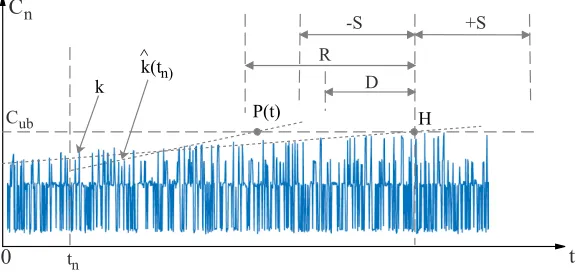
A diagram that shows the important terms and notations is given in Fig. 1. The symbols and notations we used in this experiment are listed below:

– t: the current (discrete) time; we assume t is equally spaced in time and there are no observations between two successive time pointstn−1 andtn.

– Cub: the upper bound of task execution time. During run-time if the

worst-case execution timeCmexceeds this bound, i.e.,Cm> Cub, a system failure

will occur.

– k: the actual deterministic trend that is ejected while generating a dataset. We use ˆk(t) to represent the trend magnitude that is estimated at timet. – H: H is the Hypothetical Failure Point (HFP), which is defined as the

H

tn

P(t) k

t

C

D R

-S +S

k(t_n) ^

0

Fig. 1.Representation of important notations and regions

– R: the reaction time, which is defined as the earliest time that a system should make actions before a failure happens. If a control action is made earlier than (H−R), we have a false positive.

– D:Dis the deadline before which any control action should have been made. If any action is made in the interval (H−R, H−D], we say that this estimator behaves correctly and mark the action as a true positive. Otherwise, we have a false negative if no action is made.

– P(t): is a prediction ofH made at timet; We haveP(t)→ ∞if no trend or a negative trend is found. In practice we makeP(t) =t+B, ifP(t)≥t+B, whereB is a boundary. This boundary indicates that the failure is too far away to be concerned now.

– S: the satisfactory region deviated fromHthat is used to evaluate the good-ness ofP(t). IfH−S≤P(t)≤H+S, we say the estimation is satisfactory.

During run-time, the system will continuously estimate a failure point and will only make a control action if the estimated failure point will be reached soon. Specifically, an action is taken if P(t)< t+R, or more accurately if the prediction is run every T time, then an action is made based on the criterion P(t)< t+R−T. The use of confidence intervals is not involved in this work, and each action is made independently. To evaluate the effectiveness of each algorithm, we associate positives and negatives with whether an action is taken when it should be. We have a logic table shown in Table 1.

Table 1.Definition of positives and negatives

t∈ [0, H−R) [H−R, H−D) [H−D, H) Action Made false positive true positive true positive

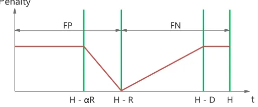
Penalty

H H - D

H - R t

FP FN

H - αR

Fig. 2.Penalties that are given to false positives/negatives

In reality, we found the numbers of false positives/negatives cannot provide enough information of the goodness of an algorithm, e.g., a false control action made close to the reaction region is at least better than the one made far earlier. Hence we introduce a penalty function (shown in Fig. 2). The penalty of false positives is decreased when the time is approaching the response region (H−R), and the penalty of false negatives is increasing from (H −R) to the deadline (H−D). The coefficientαdefines the tolerance of early actions. Whent > H−D, any false negative will score a higher penalty, as the deadline is already missed in this case.

4.2 Experiment Setup

In general, we have two groups of synthetic time-series data:A)trend-free;B) with a trend. We use the same initial worst-case execution time in both groups, and in group B we have five distinct magnitudes of trends that are gradually increasing from 1% to 4%. For each value of trend we independently generated 10 datasets, so overall we have 50 datasets. Each dataset is generated until the point where a failure would happen, which is directly calculated from the actual trend. The size of the trend-free dataset is made the same as data with 1% trend. A full list of the datasets is shown in Table 2.

Table 2.A table of generated datasets

Group Subgroup Dataset Index Data Size Increasing Trend

A A1 1 - 10 5,000 0%

B

B1 11 - 20 5,000 1%

B2 21 - 30 2,500 2%

B3 31 - 40 1,667 3%

B4 41 - 50 1,250 4%

1. Define a sampling windowW, and start to make the first estimation at time t=W.

2. Apply data selection process for samplings from (t −W) to t. Fit pre-processed time series data with each trend analysis method to generate trend models.

3. Use the models to estimate the system failure pointP(t). Make a (dummy) control action ifP(t) satisfiesP(t)−t≤R.

4. Make an evaluation of each estimation, including prediction error, valid/ invalid of the estimation and the property of the action if is made. A cumu-lative penalty is added if a false positive/negative is presented.

5. Move tot=t+M and repeat from step 2 until all data points are processed, where M is the step size. M controls the fraction of new data that is not overlapped in the training set. For example, ifM = 0.2W, at each step 20% new data will be added into the analysis.

To evaluate the quality of an estimation, we can use the knowledge of the actual failure time H. We define the failure estimation error at time t as: eh(t) =

H −P(t). If |eh(t)| ≤ S, the estimation is satisfactory (valid). Otherwise, we

recognize it as invalid. A smaller prediction error represents a better estimation, and an ideal predictor would haveeh= 0. In practice, we want to have a predictor

that would give a positive error (earlier) rather than a negative error (later), as in the former case, it gives more time for the system to process and make a reaction.

In addition to failure estimation error, we also have trend estimation error, which is calculated as:ek(t) =k−ˆk(t). Note thatekandehare correlated, butek

is more intuitive in evaluation of the precision of estimated slopes. To study the absolute performance of each algorithm, we introduce a baseline algorithm: the

Ideal Predictor (IDP), which has the foresight to know the HFP and associated time regions. For IDP, we have∀t:ek(t) = 0 and∀t:eh(t) = 0.

4.3 Results

Following the experiment steps that we defined earlier, we evaluated all combina-tions of trend identification and preprocessing methods. To have a understanding of advantages and disadvantages of different methods, we have overall three eval-uations that focus on different aspects of the results obtained from the previous experiment.

¯ ei,j,κk =

1 Nκ

Nκ

X

n=1

ei,j,κk (W+n∗M)

= 1 Nκ

Nκ

X

n=1

(k−ˆki,j,κ_(W+n∗M))

(1)

where W is the sampling window,M is the step size and Nκ is the number of

evaluations made over datasetκ. In our case, datasets with different magnitude of trends have different sizes. Hence Nκof each subgroup is distinct, which can

be calculated from:

Nκ=f loor((size of(κ)−W)/M) + 1. (2)

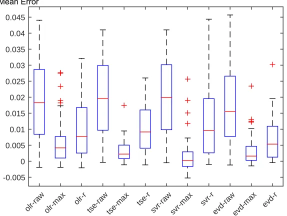
We group ¯ei,j,κk by{i, j}, and plot them out as box plots in Fig. 3. We have

overall 12 box blots (4 identification×3 preprocessing methods), and each box plot consists of 50 data points that comes from all datasets. From Fig. 3, we could clearly see that results using raw data have the worst performance, i.e.,

olr-raw, tse-raw, svr-raw and evd-raw. Compared with the other two methods

max andr, methods usingraw have a significant larger median and variance of mean errors. This is reasonable because if raw data is used in the training set, the extreme values that have trends in them will be overwhelmed by the data points with no trend. Actually as what we observed during the experiment, ˆkis approximately 0 for all raw-based methods, i.e., no trend is identified.

If we further compare block-maxima and r-largest, we can see that even con-sidering outliers, block-maxima still performs much better than r-largest across all four methods. To measure the improvement, we make pairwise comparisons for each identification method with block-maxima and r-largest. Specifically, we compare minimum, median, mean, maximum and standard deviation across all

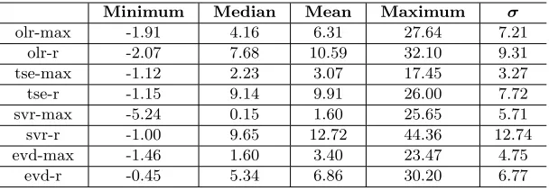
-max and-r methods. The result is shown in Table 3 (all numbers in the table are multiplied by 1×103_).

Table 3.Mean error of ˆkfor block maxima and r-largest

Minimum Median Mean Maximum σ

olr-max -1.91 4.16 6.31 27.64 7.21

olr-r -2.07 7.68 10.59 32.10 9.31

tse-max -1.12 2.23 3.07 17.45 3.27

tse-r -1.15 9.14 9.91 26.00 7.72

svr-max -5.24 0.15 1.60 25.65 5.71

svr-r -1.00 9.65 12.72 44.36 12.74

evd-max -1.46 1.60 3.40 23.47 4.75

olr-raw olr-max olr-rtse-raw tse-max tse-rsvr-raw svr-max svr-r_{evd-rawevd-max} evd-r

-0.005 0 0.005 0.01 0.015 0.02 0.025 0.03 0.035 0.04 0.045

Mean Error

Fig. 3.Distribution of mean trend errors ˆkof considered prediction methods

From the table, we can see the minimal errors are roughly the same, except

svr-max which has slightly larger error. If we look atolr-max andolr-r, we can see thatolr-r has 85% larger median, 69% larger mean and 16% larger maximal error. For tse-max and tse-r, these values are 310%, 223% and 49%. svr-max

outperformed svr-r with 69.5% improvement in mean and 1.87×10−2 less in

maxima. Considering the original trend is in a magnitude of 1×10−2(from 1% to

4%), this is a significant improvement. Finally for evd-max andevd-r, a similar conclusion is obtained: evd-max is about 100% better than evd-r in terms of mean error, and 6.73×10−3 less in maxima.

As a conclusion, compared with using raw data, data preprocessing can signif-icantly improve identification performance. It can be seen that, for our particular dataset and block size, block maxima performs the best.

Dataset Index

0 5 10 15 20 25 30 35 40 45 50

-0.01 -0.005 0 0.005 0.01 0.015 0.02 0.025 0.03

IDP-MAX OLR-MAX TSE-MAX SVR-MAX EVD-MAX

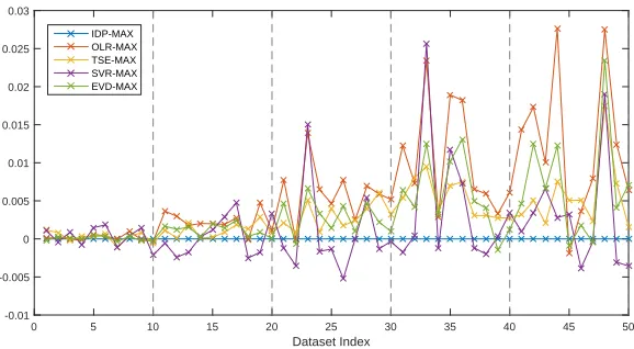
Fig. 4.Estimated trend error of each dataset. All methods use block maxima for data preprocessing. Subgroups are separated by dashed lines.

This suggests that the estimation error is highly correlated to the magnitude and characteristics of the trend.

As a conclusion, estimation error is data sensitive. With the magnitude of trend increases, the error will be increased proportionally. All of these methods are sensitive to the actual characteristic of a dataset. From Fig. 4, we can see different methods have very similar patterns in terms of peaks and troughs. This indicates that although these methods are sensitive to datasets, but as the way they vary is similar and the same dataset is used across all methods, the characteristics of the dataset will not break the fairness of this comparison. However, a large number of datasets should be used to average the variations across datasets so the actual performance can be revealed.

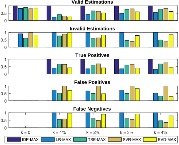
Comparison of Identification Methods In this evaluation, we will compare trend identification methods with only block maxima, as it performed the best among all data preprocessing methods. To compare the effectiveness of a trend identification method, one important index is the ability to detect a trend. In our work, this is measured by two factors: the validation of an estimation, and the positiveness of a related control action. A diagram that shows the relative performance is shown in Fig. 5. Each bar plot shows a different metric of all four methods, plus the Ideal Predictor (IDP), separated by dataset subgroups. For plots of valid and true positives, data is normalized to [0,1] by IDP, while for plots of invalid and false positive/negative, data is normalized by the worst method.

0 0.5

1 Valid Estimations

IDP-MAX LR-MAX TSE-MAX SVR-MAX EVD-MAX

0 0.5

1 Invalid Estimations

0 0.5

1 True Positives

0 0.5

1 False Positives

k = 0 k = 1% k = 2% k = 3% k = 4% 0

0.5

1 False Negatives

Fig. 5.Experiment result - normalized false negatives/positives

to give more false positives, while OLR gives more false negatives. All methods give no false positives and negatives when there is no trend in the data. TSE is consistent and has the best performance on average.

To further compare these methods, we summarize penalties that come from the results of all datasets for each method, which is shown in Table 4. From the table it can be seen that TSE has least mean penalties with all three data selection methods, comparing with the other three methods. This is identical to the conclusion we described earlier. For methods using block maxima, OLR obtained the largest penalty, while for r-largest, it is SVR.

Table 4.Mean penalties over all datasets for each prediction method

OLR TSE SVR EVD

raw 62 62 62 62

maxima 58.28 29.02 42.26 49.68

r-largest 58.2 53.82 77.58 55.76

computation, but it is sensitive to the composition of the dataset, and it will be biased if a large percentage of non-relevant data is involved. SVR is computa-tional intensive has addicomputa-tional parameters that can be tuned: the cost C that controls the trade-off between errors of the SVM on training data and margin maximization, and the epsilonǫthat controls the size of insensitive region. The ability of supporting non-linear trends is supported by SVR as well. SVR directly supports non-linear data by using Kernel functions, while other methods have to be extended to support non-linearity. In this work, we only considered one inference variable: the system duration. However if more dependent variables need to be considered, a support for multi-variable regression will be necessary, which both OLR and SVR can support while the other two cannot.

5

Conclusions

In this work, we have introduced the motivation of identifying long-term trends in worst-case execution times to achieve timing fault prediction. We have shown four different trend identification methods and compared their performance. The results suggest that data preprocessing should be used as the procedure can significantly improve estimation performance. It also can be seen that the Theil-Sen estimator, which is a non-parametric method, achieved the best per-formance in this particular experiment. It is robust against noise and outliers, and is computational effective. The other non-parametric method, SVR, is also an outstanding method as it can predict non-linear trends and can be used in multi-variable regression. Extreme value did not perform well because it needs a large amount of data to fit the distribution, i.e., a large data block. However, this will decrease the ability of early detection of failures. Finally for OLR, the performance is not satisfactory as the assumption of normally distributed resid-uals is violated. This can be improved by assuming a more accurate distribution of data, which requires to further examine the characteristics of WCET. The experiment result suggests a preference for using non-parametric methods with either block-maxima or r-largest.

For future work, we will consider more dependent variables that influence a WCET to improve the precision of prediction. The use of ensemble learning to combine two or three identification methods could also benefit the result of analysis, and multiple successive predictions should be considered to confidently make a control decision. We also aim to obtain real-life data from industrial applications, to examine if a similar result would be obtained. All these issues will form topics for future work.

References

2. Fisher, R.A., Tippett, L.H.C.: Limiting forms of the frequency distribution of the largest or smallest member of a sample. In: Mathematical Proceedings of the Cam-bridge Philosophical Society. vol. 24, pp. 180–190. CamCam-bridge Univerisity Press (1928)

3. Frei, C., Sch¨ar, C.: Detection probability of trends in rare events: Theory and

application to heavy precipitation in the Alpine region. Journal of Climate 14(7), 1568–1584 (2001)

4. Hess, A., Iyer, H., Malm, W.: Linear trend analysis: a comparison of methods. Atmospheric Environment 35(30), 5211–5222 (2001)

5. Hill, T., O’Connor, M., Remus, W.: Neural Network models for time series fore-casts. Management Science 42(7), 1082–1092 (1996)

6. Kunkel, K.E., Andsager, K., Easterling, D.R.: Long-term trends in extreme precip-itation events over the conterminous United States and Canada. Journal of Climate 12(8), 2515–2527 (1999)

7. Lu, C., Stankovic, J.A., Son, S.H., Tao, G.: Feedback control real-time scheduling: Framework, modeling, and algorithms. Real-Time Systems 23(1-2), 85–126 (2002) 8. McLeod, A.I., Hipel, K.W., Bodo, B.A.: Trend analysis methodology for water

quality time series. Environmetrics 2(2), 169–200 (1991)

9. Qi, M., Zhang, G.P.: Trend time–series modeling and forecasting with Neural Net-works. IEEE Transactions on Neural Networks 19(5), 808–816 (2008)

10. Reinsel, G.C., Tiao, G.C.: Impact of chlorofluoromethanes on stratospheric ozone: A statistical analysis of ozone data for trends. Journal of the American Statistical Association 82(397), 20–30 (1987)

11. Sen, P.K.: Estimates of the regression coefficient based on Kendall’s tau. Journal of the American Statistical Association 63(324), 1379–1389 (1968)

12. Shang, H., Yan, J., Gebremichael, M., Ayalew, S.M.: Trend analysis of extreme precipitation in the Northwestern Highlands of Ethiopia with a case study of Debre Markos. Hydrology and Earth System Sciences 15(6), 1937–1944 (2011)

13. Smith, R.L.: Extreme value analysis of environmental time series: an application to trend detection in ground-level ozone. Statistical Science pp. 367–377 (1989) 14. Smola, A.J., Sch¨olkopf, B.: A tutorial on Support Vector Regression. Statistics and

Computing 14(3), 199–222 (2004)

15. Stankovic, J.A., Lu, C., Son, S.H., Tao, G.: The case for feedback control real-time scheduling. In: Proceedings of the 11th Euromicro Conference on Real-Time Systems. pp. 11–20. IEEE (1999)

16. Tiao, G.: Use of statistical methods in the analysis of environmental data. The American Statistician 37(4b), 459–470 (1983)

17. Visser, H., Molenaar, J.: Trend estimation and regression analysis in climatological time series: An application of structural time series models and the Kalman filter. Journal of Climate 8(5), 969–979 (1995)

18. Wilhelm, R., Engblom, J., Ermedahl, A., et al.: The worst-case execution-time problemoverview of methods and survey of tools. ACM Transactions on Embedded Computing Systems (TECS) 7(3), 36 (2008)

19. Zhang, G.P., Qi, M.: Neural Network forecasting for seasonal and trend time series. European Journal of Operational Research 160(2), 501–514 (2005)