Efficient frequency response computation for loworder modelling of spatially distributed systems

This is a repository copy of

Efficient frequency response computation for loworder

modelling of spatially distributed systems

.

White Rose Research Online URL for this paper:

http://eprints.whiterose.ac.uk/130083/

Version: Accepted Version

Article:

Dellar, O. and Jones, B. orcid.org/0000-0002-7465-1389 (2018) Efficient frequency

response computation for loworder modelling of spatially distributed systems. International

Journal of Control. ISSN 0020-7179

https://doi.org/10.1080/00207179.2018.1468927

Reuse

Items deposited in White Rose Research Online are protected by copyright, with all rights reserved unless indicated otherwise. They may be downloaded and/or printed for private study, or other acts as permitted by national copyright laws. The publisher or other rights holders may allow further reproduction and re-use of the full text version. This is indicated by the licence information on the White Rose Research Online record for the item.

Takedown

If you consider content in White Rose Research Online to be in breach of UK law, please notify us by

Full Terms & Conditions of access and use can be found at

International Journal of Control

ISSN: 0020-7179 (Print) 1366-5820 (Online) Journal homepage: http://www.tandfonline.com/loi/tcon20

Efficient frequency response computation for

low-order modelling of spatially distributed systems

O. J. Dellar & B. Ll. Jones

To cite this article: O. J. Dellar & B. Ll. Jones (2018): Efficient frequency response computation for low-order modelling of spatially distributed systems, International Journal of Control, DOI: 10.1080/00207179.2018.1468927

To link to this article: https://doi.org/10.1080/00207179.2018.1468927

Accepted author version posted online: 24 Apr 2018.

Submit your article to this journal

View related articles

Publisher: Taylor & Francis

Journal: International Journal of Control

DOI: https://doi.org/10.1080/00207179.2018.1468927

MANUSCRIPT SUBMITTED TO INTERNATIONAL JOURNAL OF CONTROL

Efficient frequency response computation for low-order modelling of spatially distributed systems

O. J. Dellara _{and B. Ll. Jones}a

a

Department of Automatic Control and Systems Engineering, The University of Sheffield, S1 3JD, UK

ARTICLE HISTORY

Compiled April 23, 2018

ABSTRACT

Motivated by the challenges of designing feedback controllers for spatially distributed systems, this paper presents a computationally efficient approach to obtaining the point-wise frequency response of such systems, from which low-order models can be easily identified. This is achieved by sequentially combining the individual fre-quency responses of the constituent lower-order subsystems in a way that exploits the interconnectivity arising from spatial discretisation. Importantly, this approach extends to the singular subsystems that naturally arise upon spatial discretisation of systems governed by partial differential-algebraic equations, with fluid flows being a prime example.

The main result of this paper is a proof that the computational complexity as-sociated with forming the overall frequency response is minimised if the smallest subsystems are first merged into larger subsystems, before combining the frequency responses of the latter. This reduces the complexity by several orders of magnitude; a result that is demonstrated upon the numerical example of a spatially discretised two-dimensional wave-diffusion equation.

By avoiding the necessity to construct, store, or manipulate large-scale system matrices, the modelling approach presented in this paper is well conditioned and computationally tractable for spatially distributed systems consisting of enormous numbers of subsystems. It therefore bypasses many of the problems associated with conventional model reduction techniques.

KEYWORDS

Low-order modelling, large scale systems, spatially distributed systems, frequency response, computational efficiency, flow control.

1. Introduction

The interconnection of numerous low-order subsystems can result in large-scale sys-tems that display a dynamical wealth far in excess of their constituent parts. Ex-amples include power fluctuations within distributed power grids (Zhong & Hornik,

2013), string instabilities in traffic systems (Swaroop & Hedrick,1996) and congestion of the internet (Low et al., 2002). Such systems are also obtained upon spatial dis-cretisation of systems governed by partial differential equations (PDEs) and partial differential algebraic equations (PDAEs). These include the flexing of beams, propa-gation of sound waves, and heat transfer (Curtain & Morris,2009), and the motion of fluid flows (Aamo & Krsti´c,2003).

The focus of this paper is on obtaining low-order models of such systems for the purpose of feedback controller design. Fluid flows are of particular interest since the control of these could lead to significant economic and environmental benefits (el Hak,

2000;Bradley,2000;Kim,2011). However, control of fluid flows remains difficult since the underlying plant dynamics are, in many cases, governed by the incompressible Navier-Stokes equations; a coupled set of nonlinear PDAEs in which the algebraic con-straints arise not only from incompressibility, but also from the imposition of boundary conditions (Jones et al.,2015). Assumptions of linearity are justifiable in many cases, thereby simplifying the model to one that is linear and time-invariant (LTI), albeit still infinite-dimensional and algebraically constrained.

Methods based on infinite-dimensional linear systems theory (Curtain & Zwart,

1995) have been developed, whereby spatially distributed systems governed by PDEs

can, in some cases, be transformed into irrational transfer functions, which can then be approximated for the purposes of controller design (Curtain & Morris,2009). However, it is not clear to what extent this methodology can extend to PDAEs, particularly those in more than one spatial dimension and where the geometry of the domain is complex. If a further approximation is made based upon spatial discretisation, the model simplifies to one that is LTI, finite-dimensional and singular (Dai, 1989), with the following state-space representation:

Ex˙(t) =Ax(t) +Bu(t), (1a)

y(t) =Cx(t) +Du(t), (1b)

where u(t) _∈ Rq_{, y(t) ∈} Rp_{, x(t) ∈} Rn _{are the input, output and state vectors,}

respectively, and E_∈Rn×n_{, A ∈}Rn×n_{, B ∈}Rn×q_{, C∈}Rp×n_{, D ∈}Rp×q _are

state-space matrices. However, the state dimension will be prohibitively large from the point of view of direct synthesis of a model-based controller, hence necessitating some form of model-order reduction. For flows in simple geometries, such as plane channel flow,

further assumptions can be made to reduce the dimensionality of the system (Aamo

& Krsti´c, 2003), but for flows in complex geometries, such as over the rear face of a road vehicle, such techniques are not readily applicable.

A number of further assumptions are made in relation to (1) that whilst motivated in particular by flow control applications are nevertheless still representative of a wider class of problems. These are listed below:

A1. The pair (E,A) is regular (Dai,1989), so as to ensure existence of the transfer function of (1).

A3. The majority of subsystems arising from the spatial discretisation have no con-trol input or measured output and the number of sensors and actuators is low. Centralised, rather than distributed controllers are therefore of relevance. A4. The subsystems arising from discretisation may each possess different dynamics.

A5. Controllers based upon low-order approximations of (1) should come with a

priori guarantees of closed-loop stability/performance when applied to (1).

The second assumption immediately discounts the majority of existing methods

based upon balanced truncation or Krylov approximation of large scale systems (

An-toulas, 2005;Stykel, 2004). On the other hand, data-driven methods, such as system identification, proper orthogonal decomposition (POD) and balanced proper orthog-onal decomposition (BPOD) (Holmes et al., 1996; Rowley, 2005; Willcox & Peraire,

2002;Weller et al.,2009;Mathelin et al.,2010;Akhtar et al.,2012) are not applicable here owing to the fact that they yield models that are close to the high-dimensional system in an open-loop sense and thus may not capture the dynamics of importance from a closed-loop perspective (Curtain & Morris,2009;Jones & Kerrigan,2010) nor reflect the closed-loop objectives (Bewley et al.,2016). The other problem with data-driven methods is the need to generate the data in the first place. Physical experiments are typically expensive in terms of cost, whilst simulations can be expensive in terms of time. Other notable works on the control of spatially distributed system include that of D’Andrea & Dullerud (2003) where distributed controllers were designed for large-scale systems consisting of identical sub-systems each with sensing and actuation capabilities; a separate problem to that considered in this paper.

The techniques developed in this paper stem from the viewpoint that if the govern-ing PDAE is known, then the dynamic information within this should be exploited, rather than discarded in favour of a data driven approach. Hence, the aim of this work is to develop a computationally tractable approach to obtaining low-dimensional mod-els of PDAE systems suitable for feedback control design. Furthermore, this approach should avoid the construction of extremely large state-space matrices, or the need to generate data from experiments. It is inspired by two key works, the first of which is that of Dahan et al. (2012) who designed feedback controllers for bluff body drag

reduction. Despite Dahan’s simulation model employing in excess of _O(104) states,

open-loop harmonic excitation revealed a frequency response almost identical to that of asecond-order system owing to the fact that the vast majority of states had negli-gible influence upon the input-output response of the system. Obtaining the frequency response of a large-scale system is thus central to exposing its low-order nature, or otherwise. The second key work is that of Baramov et al.(2004), who constructed the frequency response of a 2D plane channel flow system in a point-wise fashion using the Redheffer Star Product (Doyle et al.,1991). More recent work byJones(2014) has shown how low-order models can be fitted to point-wise-in-frequency data in such a

way as to enable the derivation of an upper bound on the ν-gap (Vinnicombe,2000)

between the low-order fitted model and the full-scale system. This subsequently

en-ables the design of low-order robust feedback controllers with a priori guarantees of

robust stability and performance when connected to the full-scale system.

choice of subdomains over which to define subsystems and the subsequent order in which to combine these, is far from intuitive. If the aim is to obtain the overall fre-quency response with the least computational cost, which choices are best? This paper addresses these issues, with particular focus on the first; the optimal choice of sub-domain. The key results are that for a PDAE in two spatial dimensions, an optimal scale at which to define a subsystem exists (Proposition3.1) and that upon combining these subsystems in a prescribed sequence, the resulting complexity of computing the

system frequency response is reduced to _O ̺2(Theorem 3.2), where ̺ is the mesh

density, as compared to _O ̺4 and _O ̺6, for the extremes of smallest and largest

subsystems, respectively. In practical terms this means that the time taken to compute the frequency response of a spatially distributed system can be shortened by several orders-of-magnitude through optimal choice of domain decomposition.

The remainder of the paper is organised as follows. Section2presents an overview of the approach employed for modelling spatially distributed systems, detailing the steps required to obtain the point-wise frequency response of a system governed by PDAEs. In Section3, the domain decomposition optimisation is described, and the main results

of the paper presented. The modelling approach is demonstrated in Section4upon a 2D

wave-diffusion system. The frequency response obtained using the approach outlined in Section3 is compared to that obtained via direct construction of the full-scale system model, and relevant computational properties are discussed. Finally, conclusions and future work are presented in Section5.

2. Preliminaries on spatially distributed systems

This paper considers linear/linearised PDAEs of not more than d= 2 spatial

dimen-sions, spatially discretised using three-point finite-differences, but such assumptions are not restrictive. Hence, consider a two-dimensional and linear PDAE on spatial

domain Ω with domain boundary∂Ω, discretised in space upon a cartesian grid

con-sisting of nodes characterised by indices (i, j) in the x and y directions, respectively. Each node is thus a low-dimensional descriptor state-space models of the form:

Ei,j

d

dtxi,j(t) =Ai,jxi,j(t) +Bi,jξi,j(t) +Bui,jui,j(t), (2a) zi,j(t) =Ci,jxi,j(t), (2b) y_i,j(t) =Cyi,jxi,j(t), (2c)

where t _∈ R+ _{is time and xi,j(t) ∈} Rn _{is the node’s state vector, (assuming each}

subsystem possesses the same number of states). Note the use of bold fonts for system variables and regular fonts for spatial directions. Inputs in the form of state information from neighbouring nodes are represented by ξ_i,j(t)_∈R2dn_{, where:}

ξ_i,j(t) :=x⊤_i,j−1(t) x⊤_i+1,j(t) x⊤_i,j+1(t) x⊤_i−1,j(t)⊤_∈R4n_,

in the 2D case. The vector of control inputs is denotedui,j(t)_∈Rqi,j,_y

i,j(t)∈Rpi,j is a

vector of measured outputs and zi,j(t)_∈R2dn _{is the output of the node’s state vector}

to neighbouring nodes. The system matrices are Ei,j,Ai,j ∈ Rn×n, Bi,j ∈ Rn×2dn, Bui,j ∈ R

n×qi,j, _C i,j :=

I I _{∙ ∙ ∙} I⊤ _∈ R2dn×d _{and C}

yi,j ∈ R

the majority of subsystems will not possess control inputs or measured outputs, only nodes corresponding to the physical locations of actuation or sensing will have these.

Taking Laplace transforms of (2) with initial condition xi,j(0) = 0 yields:

˜

zi,j(s)

˜

y_i,j(s)

=

Ci,j Cy_i,j

(sEi,j−Ai,j)−1

Bi,j Bui,j

| {z }

Pi,j(s)

_˜ ξ_i,j(s) ˜

ui,j(s)

, (3)

where Pi,j(s) ∈ R(2dn+pi,j)×(2dn+qi,j), R is the space of real-rational transfer

func-tion matrices, ˜_∙ denotes a Laplace transformed quantity, and s _∈ C_{. Assuming the}

pair (Ei,j,Ai,j) is regular (Dai,1989) ensures the existence ofPi,j(s).

Being defined at the nodal level, the Pi,j are the smallest definable subsystems

and are henceforth referred to as ‘atoms’. The interconnection of neighbouring atoms

is shown in Figure 1. For a given frequency ω _∈ R_{, the frequency response of each}

atom Pi,j(iω) ∈ C(2dn+pi,j)×(2dn+qi,j) can be computed in a point-wise fashion. The

complexity associated with this computation is dominated by the LU factorisation

of (iωEi,j −Ai,j) which, in big-O notation, is O n3

flops (Golub & Loan, 1996), where one flop is defined as a single addition, subtraction, multiplication or division

between two floating point numbers (Golub & Loan, 1996). Given the small state

dimension of each atom, the point-wise evaluation of an atom’s frequency response is nevertheless extremely cheap. The remaining challenge is to combine the (point-wise) frequency response of each atom in an efficient fashion to yield the overall (point-wise) frequency response of the underlying large-scale system. As in Baramov et al.(2004), this can then be accomplished using the Redheffer star product (RHSP).

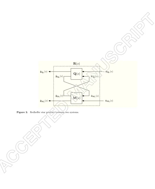
2.1. Redheffer star product

The RHSP describes the interconnection of two multi-input multi-output (MIMO) LTI

systems (Doyle et al., 1991). The block diagram of the RHSP between two arbitrary

systemsQ(s) andM(s) is depicted in Figure 2.

AssumingQ(s) and M(s) are compatibly partitioned as follows:

˜

y_Q1(s) ˜

y_Q2(s)

=

Q11(s) Q12(s)

Q21(s) Q22(s)

| {z }

Q(s)

˜

uQ1(s) ˜

uQ2(s)

, (4a)

˜

y_M1(s) ˜

y_M2(s)

=

M11(s) M12(s)

M21(s) M22(s)

| {z }

M(s)

˜

uM1(s) ˜

uM2(s)

, (4b)

where Q(s) _∈ R(aQ1+aQ2)×(bQ1+bQ2), M(s) ∈ R(aM1+aM2)×(bM1+bM2), a

Q2 =

R(aM1+aM2)×(bM1+bM2)→R(aQ1+aM2)×(bQ1+bM2) is defined as (Foia¸s & Frazho,1984):

R(s) =Q(s)⋆M(s)

:=

Q11+Q12M11(I−Q22M11)−1Q21 Q12M11(I−Q22M11)−1Q22M12+Q12M12

M21(I−Q22M11)−1Q21 M21(I−Q22M11)−1Q22M12+M22

,

(5)

which yields the overall interconnection:

˜

y_Q1(s) ˜

y_M2(s)

=R(s)

˜

uQ1(s) ˜

uM2(s)

. (6)

The overall frequency response of the PDAE system, denoted G(iω), from control

inputs ˜u(s) to measured outputs ˜y(s), is thus obtained by ‘chaining’ the individual atoms’ frequency responsesPi,j(iω) together with the RHSP:

G(iω) =P1,1(iω)⋆P2,1(iω)⋆∙ ∙ ∙⋆Pi,j(iω)⋆∙ ∙ ∙⋆Pni,nj(iω). (7)

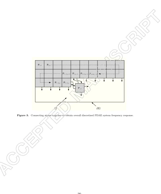
The method of subsystem chaining is shown in Figure 3 and connects atoms in a

‘snake-like’ pattern. This pattern is heuristic and it remains to be proven whether or not it leads to the lowest computational cost. However, it is guided by the complex-ity associated with the Redheffer star product operation (5). The complexity of this is dominated by the factoring of the system operators describing the mapping from interconnecting inputs and outputs. By connecting the atoms in such a fashion, the number of unconnected interconnections of the chained system remains low in com-parison to other sequences as the chaining commences, thus preventing the factored matrices in (5) from becoming excessively large.

This procedure is completed for a number of frequencies of interest, before a low-order transfer function is fitted to the frequency response using, for example, least squares regression (Hansen et al.,2012). This process lends itself to the theory devel-oped byJones (2014), where an upper bound on the ν-gap (Vinnicombe,1993,2000) between the low-order approximation and the high-order system can be computed.

This subsequently informs the design of low-order H_{∞ controllers with guarantees}

concerning the robust stabilisation of the large-scale system.

2.2. Computational complexity

The subsystem chaining method can be applied to complex geometries by embedding such geometries within a bounding rectangular (in the 2D case) computational domain. Upon spatial discretisation of the computational domain, nodal subsystems that lie outside the physical (complex) geometry can be modelled as static systems with zero direct feedthrough. When the subsystem frequency responses are chained together, all nodes in the bounding rectangular domain are included (and thus the following proofs of complexity hold), but only nodes within the complex (physical) subdomain contribute to the system frequency response. This ultimately yields the frequency response of the spatially distributed system within the physical domain.

As such, in the following analysis we assume, without loss of generality, a rectangular domain Ω := [₋ℓx/2, ℓx/2]_×[₋ℓy/2, ℓy/2]. A uniform mesh density ̺_∈N _{(nodes per}

and y directions, respectively. Assuming the snake-like chaining of subsystems shown

in Figure 3, the following lemma establishes the complexity of forming the overall

frequency response as a function of mesh density.

Lemma 2.1. The computational complexity _{C ∈}R+ _{of obtaining G(iω) isO ̺}4_.

Proof. Noting the cost of typical matrix operations as presented in Table 1,

sum-ming all the operations required to construct all ntotal = nxny atoms using (3) and

evaluate (7) yields the overall complexity:

C=_O n3_xny(1 +n)n2+ 2n2_xny(1 + 6n)n2+ 52nxnyn3, (8)

wheren_∈N_{is the state dimension of each subsystem.}

Sincenx =̺ℓx and ny =̺ℓy, for given ̺,ℓx, and ℓy, (8) can be written:

C=c1ℓ3xℓy(1 +n)n2̺4+ 2c2ℓ2xℓy(1 + 6n)n2̺3+ 52c3ℓxℓyn3̺2, (9)

wherec1, ..., c3 ∈R+ are unknown constants ofO(1). Hence the complexity is O ̺4

.

3. Optimisation by domain decomposition

The complexity of the above modelling approach can be reduced further by employing

a domain decomposition optimisation. The computational mesh is first split intonΩ =

nΩxnΩy ∈ N subdomains, defined here as computational ‘molecules’, with nΩx ∈ N

and nΩy ∈ N molecules in the x and y directions, respectively. First, the frequency

response of each molecule,PΩi,j(iω), is constructed by chaining together the individual

atoms within the molecule, using the subsystem chaining method according to:

PΩi,j(iω) =P1,1(iω)⋆P2,1(iω)⋆∙ ∙ ∙⋆Pni,nj(iω). (10)

As shown in Figure 4, the overall PDAE system frequency response G(iω) is then

obtained by connecting each of the molecule frequency responses together:

G(iω) =PΩ1,1(iω)⋆PΩ2,1(iω)⋆∙ ∙ ∙⋆PΩnΩ_x,nΩ_y(iω). (11)

For the two spatial dimension case, we now aim to prove that the the overall

com-putational complexity of evaluating G(iω) can be reduced by orders of magnitude by

optimising the domain decomposition. To begin with, the following proposition estab-lishes existence and uniqueness of values nΩx andnΩy that minimise the complexity:

Proposition 3.1. Assume mesh density ̺_≫n, lx, ly, ck, where ck _{∈ {}R_{+|ck ∼ O(1)}}

and k _∈N_{. Then there exist unique values nΩ}

x =n

⋆

Ωx and nΩy =n ⋆

Ωy that minimise the complexity of evaluating (10) and (11).

eval-uate (10) for each molecule, followed by (11) yields the overall complexity:

C=_O

n3_xn−_Ω2

xny(1 + 2n)n

2_{+ 2n}

xn−_Ωx1ny(1 + 6n)n2+ 32nxnyn3+ 4nxnyn2

+ 8nxnyn+ 16nxn−_Ω1

x+nyn

−1 Ωy

3

nΩxnΩyn

3

+ 5nΩxnΩy

nxn−_Ω1

x +nyn

−1 Ωy

2

nx₋nxn−_Ω1 x

n3

+nΩxnΩy

nxn−_Ω1

x +nyn

−1 Ωy

2

n2+nΩxnΩy nx−nxn

−1 Ωx

2

n2

+nΩxnΩy

nxn−_Ω1

x +nyn

−1 Ωy

nx₋nxn−_Ω1 x n2 . (12)

The optimal values of nΩx and nΩy which achieve the complexity reduction discussed

above are those which satisfy:

∂_C ∂nΩx

= 0 =₋2c1ℓ3xℓy(1 +n)n2n−Ωx3̺

4

−48c6ℓ2xℓyn3n−Ω2x̺

3

−32c6ℓ3xnΩyn

3_n−3 Ωx̺

3_{+ 16c}

6ℓ3yn3n−Ωy2̺

3_{+ 10c}

7ℓ2xℓyn3n−Ωx2̺

3

−5c7ℓ3xnΩyn

3_n−2 Ωx̺

3_{+ 5c}

7ℓxℓ2yn3n−Ω1y̺

3_−c 8nΩyℓ

2

xn2n−Ωx2̺

2

+ 10c7ℓ3xnΩyn

3_n−3 Ωx̺

3_+c

8ℓ2yn2n−Ωy1̺

2_+c

9ℓ2xnΩyn

2_n−2 Ωx̺

2

+c9ℓxℓyn2̺2−c10ℓ2xnΩyn

2_n−2 Ωx̺

2_+c

10ℓ2xnΩyn

2_̺2

−2c2ℓxℓy(1 + 6n)n2n−Ωx2̺

2_,

(13a)

∂_C ∂nΩy

= 0 =₋48c6ℓxℓ2yn3n−Ωy2̺

3_{+ 16c}

6ℓ3xn3n−Ωx2̺

3_{+ 5c}

7ℓ3xn3n−Ωx1̺

3

−32c6ℓ3ynΩxn

3_n−3 Ωy̺

3_{+ 5c}

7ℓxℓ2yn3n−Ωy2̺

3_+c

8ℓ2xn2n−Ωx1̺

2

−5c7ℓxℓ2ynΩxn

3_n−2 Ωy̺

3_−5c

7ℓ3xn3n−Ωx2̺

3_−c 8nΩxℓ

2

yn2n−Ωy2̺

2

+c9ℓ2xn2̺2−c9ℓ2xn2n−Ω1x̺

2_+c

10ℓ2xn2n−Ωx1̺

2

−2c10ℓ2xn2̺2+c10ℓ2xnΩxn

2_̺2_,

(13b)

which can be written as the following depressed cubic equations:

an3_Ωx+bnΩx +c= 0, (14a)

dn3_Ωy+enΩy +f = 0, (14b)

where:

a:= 16c6ℓ3yn3n−Ωy2̺

3_{+ 5c}

7ℓxℓ2yn3n−Ω1y̺

3_+c

8ℓ2yn2n−Ωy1̺

2_+c

9ℓxℓyn2̺2

+c10ℓ2xnΩyn

2_̺2_, (15a)

b:= 10c7ℓ2xℓyn3̺3−48c6ℓ2xℓyn3̺3−5c7ℓ3xnΩyn

3_̺3_−c 8nΩyℓ

2

xn2̺2

+c9ℓ2xnΩyn

2_̺2

−c10ℓ2xnΩyn

2_̺2

−2c2ℓxℓy(1 + 6n)n2̺2,

(15b)

c:= 10c7ℓ3xnΩyn

3_̺3

−32c6ℓ3xnΩyn

d:= 16c6ℓ3xn3n−Ωx2̺

3_{+ 5c}

7ℓ3xn3n−Ωx1̺

3_−5c

7ℓ3xn3n−Ω2x̺

3_+c

8ℓ2xn2n−Ωx1̺

2

+c9ℓ2xn2̺2−c9ℓ2xn2n−Ω1x̺

2_−2c

10ℓ2xn2̺2+c10ℓ2xn2n−Ωx1̺

2_+c

10ℓ2xnΩxn

2_̺2_, (16a)

e:= 5c7ℓxℓ2yn3̺3−48c6ℓxℓ2yn3̺3−5c7ℓxℓ2ynΩxn

3_̺3

−c8nΩxℓ

2

yn2̺2, (16b)

f :=₋32c6ℓ3ynΩxn

3_̺3_{. (16c)}

For _C > 0, and for all ̺, nΩx, nΩy > 0, the coefficients a and d must be positive. In

this case, sufficient conditions for the existence of global minimisers n⋆_Ωx, n⋆_Ωy to (12) in the intervals nΩx, nΩy > 0 are solutions to (14) with three distinct real roots. In

this case the roots sum to zero, meaning that at most, two roots will lie in the interval of interest nΩx,y > 0. With a, d > 0, the root with largest real part corresponds to

a minimiser of _C and is the only minimiser in the interval of interest. With respect

to (14a), existence of three distinct real roots is ensured if the following condition on the discriminant of the polynomial holds:

−4ab3₋27c2 >0. (17)

A necessary condition for (17) is b < 0. Referring to (15b), we can ensure b < 0 by selectingnΩy sufficiently large. FornΩy →̺, to leading order the coefficients (15) are:

a_{∼ O}(+nΩy̺

2_{), b∼ O(−n} Ωy̺

3_{), c∼ O(±n} Ωy̺

3_{), (18)}

thus satisfying (17). A similar argument applies to the coefficients of (14b). FornΩx → ̺, to leading order the coefficients (16) are:

d_{∼ O}(+nΩx̺

2_{), e∼ O(−n} Ωx̺

3_{), f ∼ O(−n} Ωx̺

3_{), (19)}

again satisfying the requirement that the discriminant of (14b) be positive.

We next establish how the complexity of evaluating the frequency response (11)

scales with mesh density for the case when the number of molecules are optimal. This could be achieved by solving (14) and substituting the solutions into (12). However, a more tractable solution is afforded by instead considering the following problem. For a

fixed number of molecules within the domain, let mesh density ̺ be the optimisation

variable. As this varies, so too will the size (state dimension) of the molecules. Assume the number of molecules in all directions are simultaneously optimal for a particular (optimal) value of the mesh density. Then what mesh density is required to achieve this and what is the resulting complexity? The following theorem establishes this main result.

Theorem 3.2. Given nΩx and nΩy such that nΩx =n ⋆

Ωx, nΩy =n ⋆

Ωy for ̺ =̺ ⋆_{, the}

overall complexity of evaluating (10) and (11) is_O ̺2_.

Proof. The complexity of evaluating (10) for each molecule, followed by (11), is given

by (12). Since nx =̺ℓx andny =̺ℓy, then (12) is a polynomial in ̺:

subject to the constraint that _{C ≥}0_∀̺_≥0, where:

a:=c1ℓ3xℓy(1 +n)n2n−Ωx2, (21a)

b:= 48c6ℓ2xℓyn3n−Ωx1+ 48c6ℓxℓ

2

yn3n−Ω1y + 16c6ℓ

3

xnΩyn

3_n−2

Ωx+ 10c7ℓ

2

xℓyn3

+ 16c6ℓ3ynΩxn

3_n−2

Ωy −10c7ℓ

2

xℓyn3n−_Ωx1−5c7ℓxℓ2yn3n−Ωy1+ 5c7ℓ

3

xnΩyn

3_n−1 Ωx

+ 5c7ℓxℓ2ynΩxn

3_n−1 Ωy −5c7ℓ

3

xnΩyn

3_n−2 Ωx,

(21b)

c:=c8nΩyℓ

2

xn2n−Ωx1+ 2c8ℓxℓyn

2_+c 8nΩxℓ

2

yn2n−Ω1y +c9ℓ

2

xnΩyn

2

−c9ℓxℓyn2

−c9ℓ2xnΩyn

2_n−1

Ωx+c9ℓxℓynΩxn

2_+c

10ℓ2xnΩyn

2_n−1

Ωx −2c10ℓ

2

xnΩyn

2

+ 32c3ℓxℓyn3+c10ℓ2xnΩxnΩyn

2_{+ 2c}

2ℓxℓy(1 + 6n)n2n−_Ωx1+ 4c4ℓxℓyn2

+ 8c5ℓxℓyn,

(21c)

andc1, ..., c10∈R+ are unknown constants.

The minimum complexity is achieved when:

∂_C

∂̺ =̺ 4a̺

2_{+ 3b̺+ 2c= 0, (22)}

which has solutions:

̺1=−3b

8a+ √

9b2_−32ac

8a , (23a)

̺2=−

3b

8a− √

9b2_−32ac

8a , (23b)

̺3= 0. (23c)

Since:

∂2_C

∂̺2 = 12a̺

2_{+ 6b̺+ 2c, (24)}

and_C must be increasing when ̺= 0,

∂2_C(0)

∂̺2 = 2c >0

∴c >0. (25)

Given a, c > 0, for the non-trivial roots of (22) to be physical, i.e. ̺1, ̺2 > 0, the

following must be true:

b <0. (26)

Analysis of (24), evaluated at the non-trivial roots, shows that the local minimum lies at̺⋆ _=̺

Substituting̺⋆ _{into (20) yields:}

C(̺⋆) = 9b

2_c

32a2 −

c2

4a −

27b4

512a3 +

9b3√9b2_−32ac

512a3 −

2bc√9b2_−32ac

32a2

=c̺⋆2+ 9b

3

64a2̺

⋆₊ c

4

c a+

b√9b2_−32ac

8a2

!

= ˇa̺⋆2+ ˇb̺⋆+ ˇc, (27)

where:

ˇ

a:=c, (28a)

ˇ

b:= 9b

3

64a2, (28b)

ˇ

c:= c 4

c a+

b√9b2_−32ac

8a2

!

. (28c)

Therefore for̺=̺⋆_{, the complexity (20) reduces to (27), which is O ̺}2_.

Hence, by chaining together molecules of optimal size, rather than atoms, the to-tal complexity of evaluating the frequency response of the overall system reduces

from_O ̺4 to_O ̺2 using the subsystem chaining method.

4. Application to 2D wave-diffusion equation

The effectiveness of the approach outlined above is next demonstrated upon a 2D wave-diffusion system, whose dynamics are described according to:

∂2ϕ(x, y, t)

∂t2 =c 2

1 +k∂

∂t

ϕ(x, y, t), _∀(x, y, t)_∈Ω_×[0, tf], (29)

whereϕ(_∙,_∙,_∙) : Ω_×[0, tf]_→R_{is the height of the surface,c, k∈}R+_{are constants that}

dictate the wave propagation speed and rate of diffusion, respectively, Ω := [₋2,2]_× [₋1,1]_⊂R2_{is a rectangular spatial domain with boundary∂Ω,tf ∈}R+_{is the endpoint}

of the time interval, and (x, y) _∈ Ω is a point in the domain. Periodic boundary

conditions were assumed on all boundaries, i.e.:

ϕ(2, y, t) =ϕ(₋2, y, t), _∀(y, t)_∈[₋1,1]_×[0, tf], (30a) ϕ(x,1, t) =ϕ(x,₋1, t), _∀(x, t)_∈[₋2,2]_×[0, tf], (30b)

actuation takes the form of direct control of the surface height at (x, y) = (1.5,0):

u(t) =ϕ(1.5,0, t), (31)

and sensing is a measurement of the surface height in the centre of the domain:

4.1. Full-order model

In order to derive a full-order model, the spatial domain was first discretised on a

uniform computational mesh with mesh density ̺_∈N_{in both thexand y directions.}

As such, there were nx = 4(̺−1) + 1 and ny = 2(̺−1) + 1 computational nodes in

thex andy directions, respectively, yielding a total of ntotal=nxny nodes.

Second-order spatial derivatives in both directions were approximated using second-order accurate centred finite-differences, yielding the following differentiation matrices:

D2,x:=

1 δ2 x            

−2 1 0 _{∙ ∙ ∙} 0

1 ₋2 1

0 1 ₋2 1 ...

. .. ..

. 1 ₋2 1 0

1 ₋2 1

0 _{∙ ∙ ∙} 0 1 ₋2

           

∈Rnx×nx_{, (33)}

with a similar definition for D2,y. In each case, δx = δy = δ is the (uniform) mesh

spacing in both thexandydirections. Periodic boundary conditions were implemented

by setting the (1, nx) and (nx,1) elements ofD2,x equal to one, and similarly forD2,y.

The Laplacian operator was approximated as (Trefethen,2000):

∇2 ≈L_:=In

x⊗D2,y+D2,x⊗Iny ∈R

ntotal×ntotal

, (34)

where _⊗ denotes the Kronecker product. The resulting semi-discrete approximation

of (29) is thus as follows:

E11 0

0 Intotal

| {z }

E

d dt

ϕ(t)

˙

ϕ(t)

=

A11 A12

c2L _c2_kL

| {z }

A

ϕ(t)

˙

ϕ(t)

| {z } x(t)

+Bu(t), (35a)

ysens(t) =Cx(t), (35b)

whereϕ(t)_∈Rntotal

is a vector of the values ofϕ(x, y, t) at the nodes andx(t)_∈R2ntotal is the state vector. The matricesE11,A12∈Rntotal×ntotal are identity matrices, except

for the element on the diagonal corresponding to theϕ(t) state in the actuation location being set equal to 0. Similarly, the matrices A11 ∈ Rntotal×ntotal and B ∈ R2ntotal×1

are matrices of zeros except for the element on the diagonal (respectively vertical)

corresponding to the ϕ(t) state in the actuation location, which is set equal to 1

(respectively ₋1). Lastly, C _∈ R1×2ntotal is a vector of zeros except for the column corresponding to the ϕ(t) state at the sensor location, which is set to 1. Note the algebraic constraint imposed by the actuation (31) causes E in (35) to be singular.

Whilst this full-order model is a dynamically correct representation of the wave-diffusion system, the system matrices quickly become large and ill-conditioned as the

computational mesh density is increased. The frequency response of (35) can be

com-puted for frequencies of interest ω _∈R_as:

Inverting the matrix (iωE₋A)_∈Cntotaln×ntotaln

here is particularly costly as ntotal =

nx_×ny =̺ℓx_×̺ℓy, and so the complexity of this operation is_O ̺6_{. Whilst this is}

tractable for the simple wave-diffusion equation on a relatively coarse computational mesh, and serves as a means of providing a benchmark model, it is not a practical approach in general.

4.2. Obtaining frequency response using the subsystem chaining method

Discretising (29) on the same computational mesh as the full-order model, again using second-order accurate centred finite-differences yields the following state-space repre-sentation for each atom within the domain (1_≤i_≤nx, 1≤j ≤ny):

d dt

ϕi,j(t)

˙

ϕi,j(t)

=

0 1

−4δc22 −4

c2_k

δ2

| {z }

Ai,j

ϕi,j(t) ˙

ϕi,j(t)

| {z } xi,j(t)

+Bˇi,j Bˇi,j Bˇi,j Bˇi,j

| {z }

Bi,j

ξ_i,j(t), (37a)

zi,j(t) =I I I I⊤

| {z }

Ci,j

xi,j(t), (37b)

whereϕi,j(t)_∈R_{is the value ofϕ(x, y, t) at the location of the subsystem, ξi,j(t)∈}R8

andzi,j(t)_∈R8 _{are defined as in Section 2,}

ˇ

Bi,j := 0 0 c2 δ2 c2 k δ2 ,

Ai,j ∈R2×2,Bi,j ∈R2×8, and Ci,j ∈R8×2. Each atom has the frequency response:

Pi,j(iω) =Ci,j(iωI−Ai,j)−1Bi,j ∈C8×8. (38)

The atoms describing the nodes with actuation and sensing are altered as required (these are defined in Appendix A).

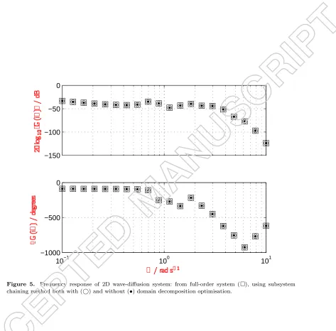
The overall system frequency responseG(iω) was obtained from (7), both with and without the use of domain decomposition optimisation. The results are presented in Figure 5 for mesh density ̺ = 25 and parameters c= 0.5 and k= 0.1. For these pa-rameters, the optimal molecule size wasn⋆

Ωx, n ⋆

Ωy

= (25,13). The frequency response

obtained from the full-order model (35) is also plotted for comparison. As expected

and despite the differences in the numerical implementations of the various methods, the subsystem chaining method produces identical frequency response data to those obtained from the full-order model, both with and without the domain decomposition optimisation.

From such frequency response data, one could then identify a low-order model and use this as the basis for designing a low-order controller.

4.3. Numerical aspects of subsystem chaining method

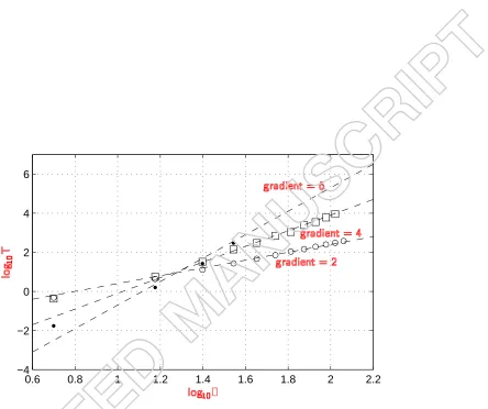
benefits of the subsystem chaining method, in terms of complexity reduction,

mem-ory usage and conditioning. Firstly, Figure 6 shows the wall-clock time T required to

compute1 G(iω) for a single frequency (ω = 1 rad s−1), as a function of mesh

den-sity ̺. It should be noted that the frequency response could not be computed from a

full-order state-space system model for mesh resolutions as high as those considered for the subsystem chaining method as the memory requirements quickly became too high.

Since the complexity is _O ̺β _{for some β ∈ R}+_{, then for large ̺ we assume the}

following relationship between wall-clock time and complexity:

T =α̺β,

∴ log₁₀T = log₁₀α+βlog₁₀̺,

where α _∈ R+ _{is some unknown constant. The gradients of the plots in Figure 6}

confirm that the complexity of computing the frequency response of a 2D system is:

• O ̺6 directly from the full-order state-space system,

• O ̺4 using the subsystem chaining method upon atoms,

• O ̺2 using the subsystem chaining method upon molecules of optimal size,

as predicted in Sections2.2–4.1.

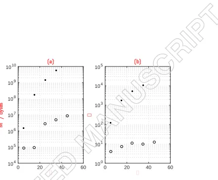
Memory requirements and numerical conditioning were analysed by considering the

memory _{M ∈} N _{(bytes) required to store the largest matrix constructed, and the}

condition number κ _∈ R+ _{(Golub & Loan, 1996) of the most ill-conditioned matrix}

that required factoring, during computation. The values of _M and κ are plotted for

increasing values of̺ in Figures 7(a) and7(b), respectively.

Both _M and κ are several orders of magnitude smaller for all ̺ considered when

using the subsystem chaining method with domain decomposition optimisation than computing the frequency response from the full order state-space system, indicating favourable computational/numerical properties of the approach.

Of course, one could improve on the performance of the simplest approach (com-puting the frequency response from the full-order state-space system) by using sparse matrices and methods (Davis, 2006), for which numerical tests revealed a complexity

of _{∼ O} ̺2.4_{. This is still more expensive than the best approach above, and}

suf-fers from large condition numbers and the difficulty of forming the full-scale system matrices in the first place.

5. Conclusions

In this paper, a computationally tractable approach to obtaining low-order linear models for the purpose of feedback control of systems governed by spatially discre-tised PDAEs was presented. The low-order nature of such systems is exposed by the frequency response, and so a method was developed for computing this by combin-ing the individual frequency responses of numerous interconnected subsystems. This avoided the need to construct, store, or operate upon the extremely large full scale system matrices that arise as a result of spatial discretisation.

For the two spatial dimension case, it was shown that the complexity of the method

1_{All computations were carried out using IEEE standard 754 double-precision floating point arithmetic on a}

was_O ̺4when combining the smallest subsystems (atoms). However, the key result of the paper established that this complexity reduced to _O ̺2by first forming larger subsystems (molecules) of optimal size, before combining these together.

The modelling approach was demonstrated by application to a 2D wave-diffusion system, and the resulting frequency response was in exact agreement with that ob-tained from a full-oder state-space model. Results were presented which showed the computational complexity scaled as predicted, and that the proposed modelling ap-proach was far better conditioned and required less memory than methods relying upon large-scale system matrices.

The method of combining subsystems assumed a snake-like sequence that was mo-tivated by heuristic argument, and so it remains to be proven that this is indeed the optimal sequence. Further future work involves applying these techniques for develop-ing controllers for flow-control problems.

References

Aamo, Ole Morten, & Krsti´c, Miroslav (2003). Flow control by feedback: Stabilization and mixing. 1st ed., London, Great Britain: Springer-Verlag.

Akhtar, Imran, Naqvi, Muntazir, Borggaard, Jeff, & Burns, John A (2012). Using dominant modes for optimal feedback control of aerodynamic forces. Proceedings of the IMechE Part G: Journal of Aerospace Engineering,227(12), 1859–1869.

Antoulas, A C (2005). An overview of approximation methods for large-scale dynamical sys-tems.Annual Reviews in Control,29, 181–190.

Baramov, Lubomir, Tutty, Owen R, & Rogers, Eric (2004).H_{∞Control of Nonperiodic}

Two-Dimensional Channel Flow.IEEE Transactions on Control Systems Technology,12(1), 111– 122.

Bewley, Thomas, Luchini, Paolo, & Pralits, Jan (2016). Methods for solution of large optimal control problems that bypass open-loop model reduction. Meccanica,51, 2997–3014. Bradley, R (2000), Technology roadmap for the 21st century truck program. Technical report

21CT-001, United States Department of Energy, Washington DC, USA.

Curtain, Ruth, & Morris, Kirsten (2009). Transfer functions of distributed parameter systems: A tutorial.Automatica,45, 1101–1116.

Curtain, Ruth, & Zwart, Hans (1995). An introduction to infinite-dimensional linear systems theory. 1st ed., New York, USA: Springer-Verlag.

Dahan, Jeremy A, Morgans, A S, & Lardeau, S (2012). Feedback control for form-drag reduc-tion on a bluff body with a blunt trailing edge. Journal of Fluid Mechanics,704, 360–387. Dai, L. (1989).Singular control systems. Lecture Notes in Control and Information Sciences,

Springer-Verlag.

D’Andrea, Raffaello, & Dullerud, Geir E (2003). Distributed Control Design for Spatially Interconnected Systems.IEEE Tranactions on Automatic Control,48(9), 1478–1495. Davis, Timothy A (2006).Direct methods for sparse linear systems. 1st ed., Fundamentals of

Algorithms, Philadelphia, PA, USA: Society for Industrial and Applied Mathematics. Doyle, John, Packard, Andy, & Zhou, Kemin (1991). Review of LFTs, LMIs and μ. In

Pro-ceedings of the 30th conference on decision and control. Brighton, England.

el Hak, Mohamed Gad (2000). Flow control: Passive, active, and reactive flow management. 1st ed., Cambridge, UK: Cambridge University Press.

Foia¸s, Ciprian, & Frazho, Arthur E (1984). Redheffer Products and the Lifting of Contractions on Hilbert Space.Journal of Operator Theory,11, 193–196.

Golub, Gene H, & Loan, Charles F Van (1996).Matrix computations. 3rd ed., Maryland, USA: The Johns Hopkins University Press.

with applications. 1st ed., Maryland, USA: John Hopkins University Press.

Holmes, P, Lumley, J L, & Berkooz, G (1996). Turbulence, coherent structures, dynamical systems and symmetry. 1st ed., Cambridge, UK: Cambridge University Press.

Jones, Bryn Ll (2014). Gap metric bound construction from frequency response data. In 19th world congress for the international federation of automatic control. Cape Town, South Africa.

Jones, Bryn Ll, Heins, Peter H, Kerrigan, E C, Morrison, J F, & Sharma, A S (2015). Modelling for robust feedback control of fluid flows. Journal of Fluid Mechanics, 769, 687–722. Jones, Bryn Ll, & Kerrigan, Eric C (2010). When is the discretization of a spatially distributed

system good enough for control?. Automatica, 46, 1462–1468.

Kim, John (2011). Physics and control of wall turbulence for drag reduction. Philosophical Transactions of the Royal Society A,369, 1396–1411.

Low, S H, Paganini, F, & Doyle, J C (2002). Internet congestion control.IEEE Control Systems,

22(1), 28–43.

Mathelin, L, Abbas-Turki, M, Pastur, L, & Abou-Kandil, H (2010). Closed-loop fluid flow control using a low dimensional model. Mathematical and Computer Modelling, 52, 1161– 1168.

Rowley, C W (2005). Model reduction for fluids, using balanced proper orthogonal decompo-sition.International Journal of Bifurcation and Chaos,15(3), 997–1013.

Stykel, Tatkana (2004). Gramian-Based Model Reduction for Descriptor Systems.Mathematics of Control, Signals, and Systems,16, 297–319.

Swaroop, D, & Hedrick, J K (1996). String Stability of Interconnected Systems. IEEE Tran-actions on Automatic Control,41(3), 349–357.

Trefethen, Lloyd N (2000).Spectral methods in matlab. Philadelphia, USA: Society for Indus-trial and Applied Mathematics.

Vinnicombe, Glenn (1993). Frequency Domain Uncertainty and the Graph Topology. IEEE Transactions on Automatic Control,38(9), 1371–1383.

Vinnicombe, Glenn (2000). Uncertainty and feedback. 1st ed., London, UK: Imperial College Press.

Weller, Jessie, Camarri, Simone, & Iollo, Angelo (2009). Feedback control by low-order mod-elling of the laminar flow past a bluff body. Journal of Fluid Mechanics,634, 405–418. Willcox, K, & Peraire, J (2002). Balanced Model Reduction via the Proper Orthogonal

De-composition. AIAA Journal,40(11), 2323–2330.

Zhong, Qing-Chang, & Hornik, Tomas (2013).Control of power inverters in renewable energy and smart grid integration. 1st ed., New York City, USA: John Wiley & Sons.

Appendix A. 2D wave-diffusion equation actuation and sensing subsystems

A.1. Actuation

The actuation node has a descriptor state-space representation:

0 0 0 1

| {z }

Eact

d dt

ϕact(t)

˙

ϕact(t)

=

−1 0

−4c2

δ2 −

4c2

k δ2

| {z }

Aact

ϕact(t)

˙

ϕact(t)

| {z } xact(t)

+

ˇ

Bi,j Bˇi,j Bˇi,j Bˇi,j

1 0

| {z }

Bact

ξ_sens(t)

u(t)

,

(A1a)

zact(t) =I I I I⊤ | {z }

Cact

with corresponding frequency response:

Gact(iω) =Cact(iωEact−Aact)−1Bact∈C8×9. (A2)

A.2. Sensing

The sensing node has a state-space representation:

d dt

ϕsens(t)

˙

ϕsens(t)

=

0 1

−4δc22 −4

c2

k δ2

| {z }

Asens

ϕsens(t)

˙

ϕsens(t)

| {z } xsens(t)

+Bˇi,j Bˇi,j Bˇi,j Bˇi,j

| {z }

Bsens

ξ_sens(t), (A3a)

zsens(t)

ysens

=

I I I I

1 0

⊤

| {z }

Csens

xsens(t), (A3b)

with corresponding frequency response:

xi,j(t₎

xi,j(t₎

xi,j(t₎

xi,j(t₎

xi−1,j(t)

xi+1,j(t)

xi,j−1(t)

xi,j+1(t) x

y

Pi,j Pi+1,j Pi−1,j

Pi,j−1

Pi,j+1

R₍s)

Q(s)

M(s) ˜

yQ1(s)

˜ y_Q

2(s)

˜ y_M1(s)

˜

y_M

2(s)

˜ u_Q1(s)

˜

u_Q

2(s)

˜ u_M1(s)

˜

u_M

2(s)

∂_Ω

Ω

P1,1 P2,1

Pi−1,j−1 Pi,j−1 Pi+1,j−1Pi+2,j−1

Pi−2,j Pi−1,j

Pi,j

∂_Ω

Ω

P_Ωi,j

P_Ωi−1,j−1 PΩi,j−1 PΩi+1,j−1

P_Ωi−1,j

P_Ω1,1 PΩ2,1

Figure 4. Connecting molecules together via domain decomposition to obtain the overall system frequency

−150 −100 −50 0

10−1 100 101

−1000 −500 0

Figure 5. Frequency response of 2D wave-diffusion system: from full-order system (), using subsystem

0.6 0.8 1 1.2 1.4 1.6 1.8 2 2.2 −4

−2 0 2 4 6

Figure 6. log of wall-clock timeT (seconds) required to obtain G(iω) for a single frequency as a function

0 20 40 60 100

101 102 103 104 105

0 20 40 60

104 105 106 107 108 109 1010

Figure 7. (a) memory M required to store largest matrix constructed during computation of frequency

Table 1. Computational complexity of matrix operations.

matrix operation big-O complexity (flops)

addition,A+B, whereA,B∈Ca×b _O

(ab) multiplication,AB, whereA∈Ca×b

,B∈Cb×c

O(abc) inversion,A−1

, whereA∈Ca×a