Experimental investigation into vibro-acoustic emission signal
processing techniques to quantify leak flow rate in plastic water
distribution pipes
J.D. Butterfield
a,d,⇑, A. Krynkin
a,d, R.P. Collins
b,d, S.B.M. Beck
c,d aDepartment of Mechanical Engineering, The University of Sheffield, Mappin St., Sheffield S1 3JD, UK b
Department of Civil and Structural Engineering, The University of Sheffield, Mappin St., Sheffield S1 3JD, UK c
Department of Multidisciplinary Engineering Education, The University of Sheffield, Leavygreave Road, S3 7RD, UK dPennine Water Group and Sheffield Water Centre, The University of Sheffield, Mappin St., Sheffield S1 3JD, UK
a r t i c l e i n f o
Article history:
Received 11 February 2016
Received in revised form 4 October 2016 Accepted 4 January 2017
Keywords: Leakage Water supply Pipeline Acoustic emission Leak rate Acoustic energy Vibration
a b s t r a c t
Leakage from water distribution pipes is a problem worldwide, and are commonly detected using the Vibro-Acoustic Emission (VAE) produced by the leak. The ability to quantify leak flow rate using VAE would have economic and operational benefits. However the complex interaction between variables and the leak’s VAE signal make classification of leak flow rate difficult and therefore there has been a lack of research in this area. The aim of this study is to use VAE monitoring to investigate signal processing techniques that quantify leak flow rate. A number of alternative signal processing techniques are deployed and evaluated, including VAE counts, signal Root Mean Square (RMS), peak in magnitude of the power spectral density and octave banding. A strong correlation between the leak flow rate and signal RMS was found which allowed for the development of a flow prediction model. The flow prediction model was also applied to two other media types representing buried water pipes and it was found that the surrounding media had a strong influence on the VAE signal which reduced the accuracy of flow clas-sification. A further model was developed for buried pipes, and was found to yield good leak flow quan-tification using VAE. This paper therefore presents a useful method for water companies to prioritise maintenance and repair of leaks on water distribution pipes.
Ó2017 The Author(s). Published by Elsevier Ltd. This is an open access article under the CC BY-NC-ND license (http://creativecommons.org/licenses/by-nc-nd/4.0/).
1. Introduction
1.1. Leaks in water distribution systems
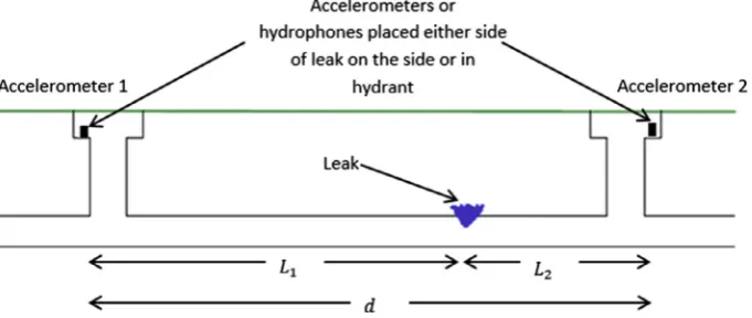
Leakage from water distribution systems (WDS) leads to a sub-stantial loss of water, which can have high negative environmental and economic effects[1]. Typically, 20–30% of water pumped into the pipe network is lost through leakage, and can be as high as 50% in developing countries and older distribution networks[2,3]. This loss of water represents a substantial amount of energy loss, as pumping and treating water has been reported to use between 2 and 3% of the worlds energy consumption[4]. In the UK, leakage alone has been estimated to cost the government £7bn annually in street works, as well as further social and damage costs[5]. Typ-ically, hydrophones or accelerometers are placed at some distance
either side of a leak (Fig. 1) and the leak’s location is found using Eq.(1):
L1¼
dc
s
delay2 ð1Þ
where d describes the distance between two accelerometers or hydrophones andcis the wavespeed of the leak noise on the pipe wall.
s
delay is the difference in signal arrival time betweenaccelerometer 1 and 2, which is calculated from the peak in the cross correlation function.
The two accelerometers receive two inputs in the form of vibra-tion,x1ðtÞandx2ðtÞ. It is possible to model the leak signal (S) and the background noise ðn1ðtÞ and n2ðtÞ) for accelerometer 1 ðx1Þ and accelerometer 2ðx2Þas:
x1ðtÞ ¼Sðt
s
1Þ þn1ðtÞ; x2ðtÞ ¼Sðts
2Þ þn2ðtÞ: ð2Þwhere
s1
ands2
describe the travel time of the leak signal arriving at both accelerometers. The majority of leak acoustic modelling studies represent background noise as Gaussian and uncorrelated between sensors (see Gao et al.[6]for example) therefore the peakhttp://dx.doi.org/10.1016/j.apacoust.2017.01.002
0003-682X/Ó2017 The Author(s). Published by Elsevier Ltd.
This is an open access article under the CC BY-NC-ND license (http://creativecommons.org/licenses/by-nc-nd/4.0/).
⇑Corresponding author at: Department of Mechanical Engineering, The Univer-sity of Sheffield, Mappin St., Sheffield S1 3JD, UK.
E-mail address:[email protected](J.D. Butterfield).
Contents lists available atScienceDirect
Applied Acoustics
in the cross correlation represents the leak. The cross correlation of the signals is described by:
Rx1x2¼E½x1ðtÞx2ðtþ
s
delayÞ; ð3ÞwhereE½is the expectation operator and
s
delaydescribes the lag intime between both received signals.
s
delayis given as:s
delay¼s
2s
1: ð4Þwhere
s
1ands
2describes the arrival time at accelerometer 1 and 2 respectively.A number of variables have been reported to influence the leak’s VAE signal received by the accelerometers, including pressure[7], flow rate [7,8], surrounding media [9], pipe material and pipe diameter[10]. Leak signals do not propagate long distances along plastic compared to metallic pipe. This is due to the viscoelastic nature of the material causing damping in the pipe wall[3], and higher frequencies tend to be attenuated or filtered as the plastic pipe acts as a low pass filter[11]. The propagation of waves in plas-tic pipes has been discussed elsewhere, for example Pinnington and Briscoe[12].
VAE still remains the most common method of leak detection in the UK and despite the ongoing research in improving the accuracy and capability of leak detection systems, the ability to classify a leak’s flow rate accurately using VAE is still not yet possible. The lack of research into the quantification of leak flow rate on WDS is likely due to the complex nature of variables influencing the leak signal; yet the accurate quantification of leak flow rate using VAE would provide an excellent tool allowing water suppliers to priori-tise maintenance thereby saving water and costs. The overall aim of this research therefore is to investigate signal processing meth-ods to classify leak flow rate on plastic water distribution pipes using VAE.
1.2. Relationship between acoustic emission and leak flow rate
Increasing WDS pressure has been demonstrated to increase leak flow rate [13], and this in turn has shown to increase the amplitude of the VAE leak signal[7,8]as well as providing a more defined peak in the cross correlation[14]. This agrees with theory that for fixed sized leaks, higher pressure results in a higher leak signal amplitude due to increased leak flow rate [15]. Similarly, Papastefanou[16]and Pal et al.[8]demonstrated increasing signal amplitude with increasing pressure due to the strong influence of leak flow rate. Pal et al.[8]also found leak flow rate increased leak VAE frequency. Papastefanou[16] established an empirical rela-tionship between leak size, amplitude and leak flow rate and con-tinued to comment that it is easier to detect leaks of a higher flow rate compared to those at lower flow rates. A study by Humphrey [14]investigated the influence of leak flow rate on correlation per-formance, finding that leaks with flow rates of 0.5 m3/h at a dis-tance of 186 m from the leak had a low success rate in detection, whereas leaks at higher flow rates of 1 m3/h at the same distance were detected more successfully. However, increasing the leak flow rate to 1.5 m3/h and increasing the measurement distance to 316 m did not produce any successful correlations [14]. The information from the literature indicates that increasing the leak’s flow rate is likely to result in an increase in leak amplitude, and it therefore seems logical to use signal parameters that will describe leak energy in order to quantify leak flow rate.
Traditionally, leak flow rateðqÞhas been shown to be sensitive to pressure through the orifice equation[17]:
q¼CdA ffiffiffiffiffiffiffiffi
2gh
p
ð5Þ
where gis acceleration due to gravity,Cd is the discharge
coeffi-cient, hole areaðAÞ, pressure headðhÞandqis the flow rate through the leak. The equation can be simplified for the application of water distribution pipes and can be written as[17]:
Nomenclature
s
delay difference in signal arrival time between accelerometer 1 & 2 (s)x1ðtÞ;x2ðtÞ VAE signals at accelerometer 1 & 2 d distance between accelerometer 1 & 2 (m) c wavespeed of propagating acoustic signal (m/s) L1;L2 distance between leak and accelerometers (m) Rx1x2 cross correlation between leak signals
E½ expectation operator
q leak flow rate (l/min) Cd discharge coefficient
g acceleration due to gravity (m/s2) h head (m)
[image:2.595.132.473.597.741.2]a
exponent due to discharge X½k discrete Fourier Transform C leakage coefficientq¼Cha ð6Þ
whereCis the leakage coefficient and
a
is an exponent of discharge and can vary due to leak hydraulics, pipe material, surrounding media and pressure[17].1.3. Previous attempts to quantify leak flow rate
Few attempts have been made to quantify a leak’s flow rate in WDS pipes using VAE, but there are some examples utilising meth-ods other than VAE. Mashford et al.[18]demonstrated a relatively high degree of accuracy predicting a leak’s size using EPANET mod-elling software and support vector machine. Salam et al.[19] con-tinued to use EPANET modelling to classify leaks according to their size. Daoudi et al.[20]used wavelet analysis and artificial neural networks to classify leak size. Collecting 55 signals from iron and PVC pipe, they managed to distinguish between large and small leaks but did not demonstrate any convincing results.
Although there have been limited studies in the water industry, there have been several successful trials in other disciplines, and these can be divided into analytical methods based on known rela-tionships between parameters and data driven comparative meth-ods such as pattern recognition [21] and spectral comparison methods. Kim et al.[22]and Na et al.[23]both used fuzzy neural networks to classify leak flow rate caused by breaks in nuclear power plants. An investigation into a leaking steam ball valve and water ball valve by Yan et al.[24]demonstrated that signal amplitude is directly proportional to leakage rate. Khulief et al. [25]found that it was easier to detect differences in sound power levels using signal root mean square (RMS) when power levels are similar, when using acoustic emission of leaks in plastic pipes. Mel-and et al.[21]found a good relationship between leak flow rate and signal RMS from leaky shut down valves in the oil and gas industry. Kaewwaewnoi et al. [26,27] and Chen et al.[28] used VAE to investigate leak flow rate classification from gas leaks and hydraulic seals respectively, and both found good correlations between signal Root Mean Square and leak flow rate of a sample containingNsamples,x½0;x½1;. . .;x½N1
RMS¼ 12X
N1
n¼0 x½n2
!0:5
ð7Þ
The work by these authors shows that the VAE signal RMS can be related to the signal’s energy content[28]. Kaewwaewnoi et al. [27]continued to develop an equation to relate VAE signal RMS from gas valve leakage to leak flow rate, although this was devel-oped specifically for valve leakage in gas systems. Chen et al. [28] compared RMS with several other several signal-energy related parameters to quantify gas leak rate, including VAE counts and the magnitude of the peak in the power spectral density (PSD). Due to the success of the techniques presented in Chen et al.[28], similar methods are employed in this research. VAE counts is determined by setting a given threshold (for integrated electronic piezoelectric accelerometers the units would usually be in volts) and counting the number of times this threshold is exceeded. As leak flow rate is related to signal amplitude [7,8,16], it can be expected that higher leak flow rates result in a higher number of VAE counts. Mba[29]found good use of simple parameters such as VAE counts and RMS to detect defects in bearings within rota-tional machines. VAE counts are also a function of the sensor, damping characteristics of the material, signal amplitude and the chosen threshold level[30]. As a result, VAE counts are less appli-cable to the wider water industry due to the variety of sensors used to record leak signals. As leak signals are continuous signals[28]
(i.e. non transient), the leak signal PSD can be used to represent the power of signals over different frequencies, and is defined by Marple[31]as:
P½k ¼T NjX½k
2
j ¼T
N
XN1
n¼0
x½nexp j2
p
kn N 2;06k6N1; ð8Þ
wereP½krepresents the PSD,Tis the sampling period andX½kis the Discrete Fourier Transform of the recorded signalx½n. Chen et al. [28]demonstrated that the magnitude of the peak in the PSD can be related to leak flow rate.
Other frequency domain methods such as octave banding can demonstrate the contribution of signal energy within given fre-quency bands and therefore may provide an alternate way of visu-alising leak flow rate in the frequency domain. Octave bands are commonly used in the description of VAE measurements, where the VAE is divided into several bands depending on the signal mag-nitude across frequency bands [32]. The bands are commonly referred to by their centre frequency, which is the average of the upper and lower frequencies so that the centre frequency equals
ffiffiffiffiffiffiffiffiffiffiffiffiffiffiffiffiffiffiffiffiffiffiffiffiffiffiffiffiffiffiffiffiffiffiffiffiffiffiffiffiffiffiffiffiffiffiffiffiffiffiffiffiffiffiffiffiffiffiffiffiffiffiffiffiffiffiffiffiffiffiffiffiffiffi
lower frequencyupper frequency
p
. The majority of leak signals on plastic pipe have been demonstrated to be low frequency: Pal et al.[8]recorded leak frequencies of 20–250 Hz on leaks from MDPE pipe, Hunaidi and Chu[7]found leak signals on plastic pipe between 50 and 150 Hz using accelerometers on a buried test rig in Canada. Muggelton et al.[33]and Papastafaneou et al.[16] demon-strated leak signals well below the pipe ring frequency. Khulief et al.[25]found the production of broadband signals at the leak source, but many of these frequencies are quickly attenuated on the pipe wall[34], or lost to the surrounding media[3], resulting in lower frequency signals. Evidently, the literature suggests that leak signals from plastic pipe span the range of 20–500 Hz and therefore would lie in octave bands between centre frequencies 31.5 Hz and 500 Hz. Hunaidi and Chu[7]suggested that the fre-quency content did not differ significantly between leak types, so therefore it is possible that the leak signals of different leak types would occur in a similar frequency range and therefore grouping by octave bands represents a good way to investigate the influence of leak signals.
2. Experimental methods, data acquisition and signal processing
A 140 m long, 50 mm internal diameter Medium Density Poly-ethylene (MDPE) pipe loop known as the Contaminant into Distri-bution (CID) systems pipe rig (Fig. 2andTable 1) at the University of Sheffield, UK[35]was used to study the influence of media and flow rate on the leak signals. A 3.5 kW variable speed pump drives water from an upstream reservoir and water recirculates around the pipe rig continuously. 3 pressure sensors (Gems 2200) were linked to a National Instruments DAQ board and LabVIEW software was used in order to process pressure data and system flow was recorded using an electromagnetic flow meter (Arkon Flow System Mag 900). The pressure sensors were used to solely measure sys-tem pressure and therefore were not used to measure the location of the leak.
placed on the flange plate 36 cm next to the leak and recorded VAE signals at 4864 Hz for 60 s in accordance with the Nyquist sam-pling theorem. Due to the nature of the fittings, the accelerometers had to be placed horizontally. However, due to the strong coupling of the pipe wall and the fluid borne axis-symmetric wave[3]which dominates the leak noise in plastic pipes, there will always be a high degree of radial motion[12,33], were energy dissipates in around the pipe wall. Therefore, the orientation of the sensor should not matter to the recorded signal. The position of the accelerometers on the flange plate was also noted and the accelerometers were positioned in the exact same place for each test for reproducibility. Accelerometer signals were passed through an anti-aliasing filter, amplification and signal conditioning unit. The accelerometer has a built in DAQ system, and at the end of the measurement procedure the data is download to a laptop com-puter and processed using MATLAB. Signals were passed through a Hanning window and 10th order Butterworth filters in order to remove frequencies greater than 1000 Hz. Signal averaging was conducted in the frequency domain. The general measurement and analytical procedure is described inFig. 3.
The pump speed was increased in order to increase system pressure and leak flow rate. Prior to the introduction of the leak, signals were measured at the different pump speeds so signals could be compared to a ‘no-leak’ scenario, where only background noise and pump noise exist, allowing for easier identification and
more accurate characterisation of the leak signal (i.e. leak vs. no-leak).
The leak was initially discharged to atmosphere whilst develop-ing the signal processdevelop-ing technique to quantify leak flow rate. In order to assess the influence of different external media types, tests were repeated with the pipe submerged to represent an idealised fluidised bed and with a geotextile fabric of 5 mm thickness (STA-BLEMASS 115) to represent a fully constrained porous media. A similar geotextile fabric was utilised in previous research by Fox et al. [37], and was found to represent an idealised unfluidised external media as the boundary condition is fully constrained therefore mobilisation of particles will not occur during fluidisa-tion. The geotextile fabric was wrapped around the leak and pipe three times for each test and was wrapped all the way to the end of the container.
3. Results and discussion
3.1. Identification of leak signals
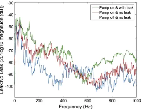
In order to fully characterise the leak noise, measurements of the system where initially taken in three states: pump off; pump on and no leak; and pump on with a leak. These results are shown
inFig. 4, which demonstrates the contribution of these sources to
[image:4.595.131.470.67.333.2]the measured signals. Background noise was most dominant at fre-quencies <50 Hz. It can be noted that both the pump and the leak contribute to the measured signal when compared to the back-ground noise. The pump appears to produce signals dominated by low frequency components between, which are most powerful at frequencies <400 Hz. Results show that the contribution of the leak noise is greatest at the lower frequencies (between 0 and 410 Hz), well below the pipe ring frequency, which agrees with the majority of the literature for leaks on plastic pipes [8,9,34]. Ring frequency is estimated to be in the vicinity of 20 kHz based on Eq. (26) in Muggleton et al.[33]. Interestingly, the background
Fig. 2.(a) Schematic of the pipe test rig. A-pump; B-pump butterfly valve; C-pump flow meter; D-pump pressure sensor; E-upstream test section butterfly vale; F-Test section pressure sensor; G-Test section pressure sensor; H-downstream flow control valve; I-downstream flow meter. (b) Photograph of test rig.
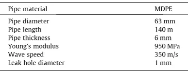
Table 1
Pipe and leak details.
Pipe material MDPE
Pipe diameter 63 mm
Pipe length 140 m
Pipe thickness 6 mm
Young’s modulus 950 MPa
Wave speed 350 m/s
[image:4.595.71.265.398.471.2]noise, pump and leak all showed similar spectra between 490 and 600 Hz. At frequencies >600 Hz, both the pump and leak noise can be separated from the background noise. However, the leak noise is shown to have amplitude signals in this range compared to the pump noise. Both the pump and the leak are therefore shown to influence the recorded signal.
During the tests, five different flow rates were investigated. The narrowband frequency spectrum for the ratio between leak and no-leak measurements at two different leak flow rates is illustrated
inFig. 5. The ratio between leak and no-leak demonstrates the
vis-ibility of the leak noise in the frequency domain at two different leak flow rates. Those magnitudes recorded at >0 dB are due to the leak noise and those signals around the zero dB mark represent either signals related to the pump or background noise. Increasing leak flow rate increased signal amplitude at specific frequencies for all five leak flow rates monitored. Notably, the frequency range 63– 280 Hz and 920–1050 Hz showed higher amplitude at higher leak flow rate. However, those frequencies ranging from 280 to 920 appeared to be less affected by leak flow rate. The highest ampli-tude signal was recorded at the highest leak flow rate of 1.7 l/min.
3.2. Leak flow rate classification methods
Considering the results shown inFig. 5and a number of authors have demonstrated a leak’s flow rate to increase signal amplitude [7,8,16], it is logical to investigate parameters that describe leak
energy in order to estimate leak flow rate using VAE. This section compares four methods that have been shown by authors to describe signal energy in other disciplines. Initially, the signal pro-cessing methods will be developed with the pipe discharging into air.
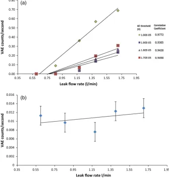
3.2.1. Vibro-acoustic emission counts vs. leak flow rate
[image:5.595.117.466.68.238.2]The accelerometer used in this study recorded outputs in raw voltage form, and the number of volts is proportional to the ampli-tude of the leak signal. The VAE count rate is defined in this mea-surement as the number of samples (VAE counts) that exceed a given voltage threshold. All VAE count rates are expressed as counts per second, thus VAE counts were divided by the signal duration in seconds. As this measurement is used very rarely in the field of leak detection on water distribution pipes, no guideli-nes exist as to the choice of threshold[28]. Similar to Chen et al. [28]different thresholds were tried and the threshold which pro-duced the best results was 1.9105V (Fig. 6a), which provided a good correlation with leak flow rate. In order to assess a change in threshold, a floating threshold was used (Fig. 6b), whereby the RMS value of the signal in question was used to set the threshold of VAE count. Similar to Chen et al.[28], using RMS as a floating threshold for VAE counts did not perform well and is not suitable for quantifying leak flow rate.
Fig. 3.Flow chart of methodological process.
[image:5.595.46.272.272.447.2]Fig. 4.Comparison of background noise, pump noise and leak signals.
[image:5.595.312.542.274.452.2]3.2.2. Root mean square vs. leak flow rate
In accordance with Eq. (7) the signal RMS for different flow rates were calculated and a strong correlation between RMS and leak flow rate is observed inFig. 7. Higher leak flow rates achieved higher RMS values compared to lower leak flow rates. The increase in RMS at the higher flow rates is likely due to an increased velocity and turbulence at the leak hole[27], and clearly demonstrates that RMS is a more suitable method for leak flow rate quantification compared to that of VAE counts (Fig. 6a and b).
3.2.3. Magnitude of peak in power spectral density vs. leak flow rate The PSD of leak signals at different flow rates is shown inFig. 8, with higher leak flow rates causing an increase in amplitude across specific frequency bands. The magnitude of the peak frequency in the PSD was tested to observe any correlation between leak flow rate and the magnitude of the peak frequency.Fig. 8indicates no significant correlation between the peak magnitude of the PSD and leak flow rate exist. This method is therefore not useful in quantifying leak flow rate compared to the other methods 0.00
0.10 0.20 0.30 0.40 0.50 0.60 0.70 0.80
VAE counts/second
Leak flow rate (l/min)
0 0.002 0.004 0.006 0.008 0.01 0.012 0.014 0.016
0.35 0.55 0.75 0.95 1.15 1.35 1.55 1.75 1.95
0.35 0.55 0.75 0.95 1.15 1.35 1.55 1.75 1.95
VAE counts/second
Leak flow rate l/min
(a)
[image:6.595.133.469.71.423.2](b)
Fig. 6.VAE counts above a given voltage threshold; (a) manually set threshold and (b) floating threshold using RMS value. Error bars denote standard deviation.
0 5 10 15 20 25
0.35 0.55 0.75 0.95 1.15 1.35 1.55 1.75
RMS (mV)
Leak flow rate (l/min)
[image:6.595.134.470.582.738.2]investigated. The poor correlation observed inFig. 8is likely due to the observed changes in leak frequency and amplitude of these peak frequencies with leak flow rate (Fig. 5), and so there is no relationship between the amplitude of the peak frequency and leak flow rate.
[image:7.595.126.460.69.267.2]3.2.4. Octave bands vs. leak flow rate
Fig. 9a shows the ratio between leak and no-leak measurements divided into octave bands. Octave bands show the intensity of the
signal in certain frequency bands known as octaves, and the results demonstrate that the majority of leak energy is located in the first 4 octaves. The second octave band (centre frequency 125 Hz) appears to have similar magnitude for all leak flow rates. The divi-sion in magnitude becomes greatest in the 4th octave (i.e. the high-est contribution of the leak noise is in the 4th octave, centre frequency of 500 Hz). The ratio of octave band 4 and 2 appears to describe leak flow rate well and could be a potential method to quantify leak flow rate (Fig. 9b).
0 5 10 15 20 25 30
0.35 0.55 0.75 0.95 1.15 1.35 1.55 1.75
Magnitude of
PSD
(m
V)
Leak flow rate (l/min)
Fig. 8.Magnitude of the peak in the PSD vs leak flow rate. Error bars denote standard deviation.
0 0.5 1 1.5 2 2.5 3
0.35 0.55 0.75 0.95 1.15 1.35 1.55 1.75 1.95
Rao of octave band (unitless)
Leak flow rate (l/min)
(a)
[image:7.595.124.464.408.729.2](b)
3.2.5. Comparison of methods
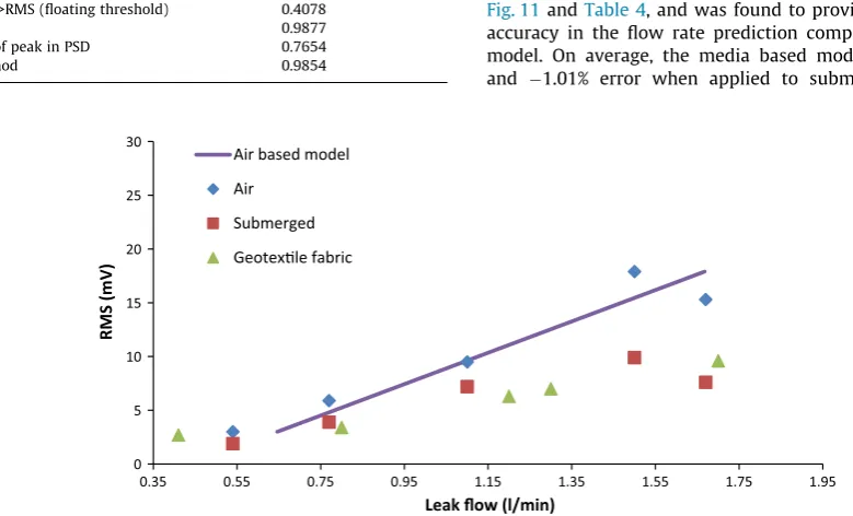
All methods except for VAE counts and the magnitude of the peak in PSD with floating threshold achieved high correlations with leak flow rate and therefore appear to be good methods in quantifying leak flow rate using VAE (Table 2). The best performing method was that of RMS and this could provide good accuracy in predicting a leak flow rate. To quantify leak flow rate using VAE an RMS model with a leak discharging into air was derived in the following form:
RMS based modelðdischarging to airÞ
QRMS¼0:0686mVRMSþ0:4406 ð9Þ
whereQRMSis the flow rate leak flow rate (l/min) based on the RMS
value andmVRMSis the received RMS value (mV). In order to assess
the applicability of this model, the pipe was submerged in water and a geotextile fabric in order to represent idealised surrounding media. The results for this model are demonstrated inFig. 10.
The accuracy of the flow prediction model based on leaks dis-charging to air is demonstrated inFig. 10and Table 3, and was found to be affected by media type. For both the submerged pipe and the pipe wrapped in geotextile fabric, the model tended to per-form well at lower flow rates but error margins became greater as the flow rate was increased. Overall, the accuracy of this model was generally poor when the media type was changed; highlight-ing a strong influence of the surroundhighlight-ing media. When the pipe was submerged, the air based model on average over-predicted leak flow rates by 37.96%, but at higher flow rates this error increased to50.33%. When the pipe was covered in geotextile fabric, the model also tended to over-predict, on average by 37.33%. These results indicate that the surrounding media has a strong influence on the leak signal and therefore a model designed on data discharging into air will yield inaccurate results in a real life buried WDS.
The resulting over-prediction of the air based model highlights the strong influence of surrounding media on the leak signal and the difficulty obtaining representative samples in a laboratory environment. This has also been highlighted by several other authors, who note a strong influence of the surrounding media on the leak signal [7,9,38,39]. The air based model performed poorly when the media type was changed due to lower RMS values in buried pipes. The reasons for the reduced RMS values within the submerged and geotextile samples are likely to be due to the extent of the impedance mismatch between the pipe and the sur-rounding media. When the leak discharges into air, the impedance mismatch is higher than when submerged and with geotextile fab-ric and therefore less leak energy is radiated into the surrounding environment. A lower impedance mismatch is present when sub-merging the pipe and wrapping it with geotextile fabric, where a low impedance mismatch generally represents efficient energy transfer[40], which will likely result in reduced leak signal energy recorded by the accelerometers.
Due to the strong influence of media on the leak’s VAE signal and resulting over-prediction of the air based model, a further flow prediction model was derived (Eq.(10)), which is based on exper-imental data taken for the submerged pipe and the pipe wrapped in geotextile fabric. In order to verify this media based model, the experimental tests were conducted once more, where the pipe was resubmerged and wrapped in geotextile fabric. This data is now referred to asvalidation dataand its purpose is to assess the accuracy of the media based model on new data sets.
RMS based modelðdischarging to mediaÞ
QRMS¼0:15127 mVRMSþ0:19893 ð10Þ
[image:8.595.313.563.96.139.2]The performance of the media based model is further plotted in
Fig. 11andTable 4, and was found to provide a higher degree of
accuracy in the flow rate prediction compared to the air based model. On average, the media based model caused only 4.17% and 1.01% error when applied to submerged and geotextile
Table 2
Comparison of different methods to quantify leak flow rate.
Leak flow rate identification parameter Correlation coefficient
VAE counts >threshold (fixed) 0.9806 VAE counts >RMS (floating threshold) 0.4078
RMS 0.9877
Magnitude of peak in PSD 0.7654
Octave method 0.9854
0 5 10 15 20 25 30
0.35 0.55 0.75 0.95 1.15 1.35 1.55 1.75 1.95
RMS (mV)
Leak flow (l/min) Air based model
Air
Submerged
Geotexle fabric
Fig. 10.Performance of the flow prediction model for leak flow rate prediction tested under different media types (discharging to air, submerged and wrapped in geotextile fabric).
Table 3
Prediction error of the leak flow rate prediction model when applied to different media types.
Submerged pipe (%) Geotextile fabric (%)
[image:8.595.89.479.494.730.2]secondary validation test data respectively. This suggests that the geotextile and submerged media types share similar RMS values, and therefore this model may be appropriate on real buried water distribution networks and could potentially be used on a wide vari-ety of WDS due to a negligible effect of media type on the model
4. Conclusions
The purpose of this work was to investigate whether it is possi-ble to derive a signal processing method which may help to quan-tify leak flow rate from leaks on plastic water distribution pipes using VAE. A variety of methods were tested and the most promis-ing method was the use of the RMS value and from this value it was possible to derive a model based on experimental data with a leak discharging into air. The air based model was found to over-predict the leak flow rate when the pipe was buried under different media types representative of a real buried WDS, due to the strong influ-ence of surrounding media on the leak’s VAE signal. This highlights the importance of media in deriving information from leaks under different media types, and laboratory samples discharging into air are unlikely to result in representative signals of leaks on a real buried water distribution network. However, when comparing the two other media types with each other, the media type was found to have a negligible influence on RMS levels and therefore a second flow prediction model was developed based on the media data. This media based model was validated for a second time on the test rig and demonstrated high levels of accuracy in quantify-ing leak flow rate. However future research is required to validate this on a real WDS with different media and leak types. The results presented in this paper demonstrate a signal processing technique to quantify leak flow rate using VAE, which will provide a useful method for water companies to prioritise maintenance and repair of leaks in WDS.
Acknowledgements
The authors would like to thank Northumbrian Water, Severn Trent Water, Thames Water Utilities, Scottish Water and the EPSRC – United Kingdom under grant number EP/G037094/1 for their funding and help with this research. The authors would also like to thank Primayer Ltd. for the loan of equipment.
Appendix A. Supplementary material
Supplementary data associated with this article can be found, in the online version, athttp://dx.doi.org/10.1016/j.apacoust.2017.01. 002.
References
[1] Colombo AF, Karney BW. Energy and costs of leaky pipes: toward comprehensive picture. J Water Resour Plan Manage 2002;128:441–50.
http://dx.doi.org/10.1061/(ASCE)0733-9496.
[2] AWWA. Leaks in water distribution systems – a technical/economic overview. Denver; 1987.
[3] Almeida F, Brennan M, Joseph P, Whitfield S, Dray S, Paschoalini A. On the acoustic filtering of the pipe and sensor in a buried plastic water pipe and its effect on leak detection: an experimental investigation. Sensors 2014;14:5595–610.http://dx.doi.org/10.3390/s140305595.
[4] de Almeida FCL, Brennan MJ, Joseph PF, Dray S, Whitfield S, Paschoalini AT. Measurement of wave attenuation in buried plastic water distribution pipes. Strojniški Vestn – J Mech Eng 2015;60:298–306. http://dx.doi.org/10.5545/sv-jme.2014.1830.
[5] McMahon W, Burtwell MH, Evans M. Minimising street works disruption: the real costs of street works to the utility industry and society. Tech rep 05/WM/ 12/8. London, UK; 2005.
[6] Gao Y, Brennan MJ, Joseph PF. A comparison of time delay estimators for the detection of leak noise signals in plastic water distribution pipes. J Sound Vib 2006;292:552–70.http://dx.doi.org/10.1016/j.jsv.2005.08.014.
[7] Hunaidi O, Chu WT. Acoustical characteristics of leak signals in plastic water distribution pipes. Appl Acoust 1999;58:235–54.http://dx.doi.org/10.1016/ S0003-682X(99)00013-4.
[8]Pal M, Dixon N, Flint J. Detecting & locating leaks in water distribution polyethylene pipes. In: World Congr Eng [II].
[9] Muggleton JM, Brennan MJ. Leak noise propagation and attenuation in submerged plastic water pipes. J Sound Vib 2004;278:527–37.http://dx.doi. org/10.1016/j.jsv.2003.10.052.
[10] Hunaidi O, Wang A. Networks acoustic methods for locating leaks in municipal water pipe networks; 2004. p. 1–14.
[11] Gao Y, Brennan MJ, Joseph PF, Muggleton JM, Hunaidi O. A model of the correlation function of leak noise in buried plastic pipes. J Sound Vib 2004;277:133–48.http://dx.doi.org/10.1016/j.jsv.2003.08.045.
[12]Pinnington RJ, Briscoe AR. Externally applied sensor for axisymetric waves in fluid filled pipe. J Sound Vib 1994;173:503–16.
0 2 4 6 8 10 12
0.35 0.55 0.75 0.95 1.15 1.35 1.55 1.75 1.95
RMS mV
Leak flow (l/min) Media based flow predicon model
Submerged
Geotexle fabric
Submerged validaon
[image:9.595.127.461.65.257.2]Geotexle fabric validaon data
Fig. 11.Performance of the media based flow prediction model for leak flow rate quantification tested on validation data.
Table 4
Prediction error using the media based model, based on the assessment of secondary validation data.
Submerged pipe (%) Geotextile fabric (%)
[image:9.595.33.285.328.373.2][13] Miller R, Pollock A, Watts D, Carlyle J, Tafuri a, Yezzi J. A reference standard for the development of acoustic emission pipeline leak detection techniques. NDT E Int 1999;32:1–8.http://dx.doi.org/10.1016/S0963-8695(98)00034-6. [14] Humphrey N. Leak detection on plastic pipes; 2012.
[15] Ver Istvan, Beranek L. No Title. Noise Vib Control Eng Princ Appl, 2nd ed.; 2005. p. 976.
[16]Papastefanou A. An experimental investigation of leak noise from water filled plastic pipes. Soc Sci 2011.
[17] Greyvenstein B. An experimental investigation into the pressure-leakage relationship of some failed 2004; 2004.
[18] Mashford J, De Silva D, Marney D, Burn S. An approach to leak detection in pipe networks using analysis of monitored pressure values by support vector machine. NSS 2009 – Netw Syst Secur 2009:534–9.http://dx.doi.org/10.1109/ NSS.2009.3.
[19] Salam AEU, Selintung M, Maricar F. On-line monitoring system of water leakage detection in pipe networks with artificial intelligence; 2014, vol. 9, p. 1817–22.
[20] Daoudi A, Benbrahim M, Benjelloun K. An intelligent system to classify leaks in water distribution pipes; 2005, vol. 4, p. 4–6.
[21] Meland E, Henriksen V, Hennie E, Rasmussen M. Spectral analysis of internally leaking shut-down valves. Meas J Int Meas Confed 2011;44:1059–72.http:// dx.doi.org/10.1016/j.measurement.2011.03.004.
[22] Kim DY, Yoo KH, Kim JH, Na MG, Hur S, Kim C. Prediction of leak flow rate using fuzzy neural networks in severe post-LOCA circumstances; 2014, vol. 61, p. 3644–52.
[23] Na M, Shin S, Jung D, Kim S, Jeong J, Lee B. Estimation of break location and size for loss of coolant accidents using neural networks. Nucl Eng Des 2004;232:289–300.http://dx.doi.org/10.1016/j.nucengdes.2004.06.007. [24] Yan J, Heng-hu Y, Hong Y, Feng Z, Zhen L, Ping W, et al. Nondestructive
detection of valves using acoustic emission technique 2015; 2015.http:// dx.doi.org/10.1155/2015/749371.
[25] Khulief YA, Khalifa A, Ben Mansour R, Habib MA. Acoustic detection of leaks in water pipelines using measurements inside pipe. J Pipeline Syst Eng Pract 2012;3:47–54.http://dx.doi.org/10.1061/(ASCE)PS.1949-1204.000008.
[26]Kaewwaewnoi W, Prateepasen A, Kaewtrakulpong P. A study on correlation of ae signals from different ae sensors in valve leakage rate detection. ECTI Trans Electr Eng Electron Commun 2007:113–7.
[27] Kaewwaewnoi W, Prateepasen A, Kaewtrakulpong P. Investigation of the relationship between internal fluid leakage through a valve and the acoustic emission generated from the leakage. Meas J Int Meas Confed 2010;43:274–82.http://dx.doi.org/10.1016/j.measurement.2009.10.005. [28] Chen P, Chua PSK, Lim GH. A study of hydraulic seal integrity. Mech Syst Signal
Process 2007;21:1115–26.http://dx.doi.org/10.1016/j.ymssp.2005.09.002. [29]Mba D. Acoustic emissions and monitoring bearing health. Tribiol Trans
2003;46:447–51.
[30] Grosse CU, Ohtsud M. Acoustic emission testing; 2008.
[31]Marple L. Digital spectral analysis: with applications. London: Prentice-Hall International; 1987.
[32]Hansen CH. Fundamentals of acoustics. Adelaide: University of Adelaide; 1994. [33] Muggleton JM, Brennan MJ, Pinnington RJ. Wavenumber prediction of waves in buried pipes for water leak detection. J Sound Vib 2002;249:939–54.http:// dx.doi.org/10.1006/jsvi.2001.3881.
[34]Brennan M, Joseph P, Muggleton J, Gao Y. The use of acoustic methods to detect water leaks in buried water pipes. Unpubl Res Rep 2006:1–7. [35] Collins RP, Boxall JB, Karney BW, Brunone B, Meniconi S. How severe can
transients be after a sudden depressurization? J Am Water Works Assoc 2012;104:67–8.http://dx.doi.org/10.5942/jawwa.2012.104.0055.
[36] Ferrante M, Massari C, Brunone B, Meniconi S. Leak behaviour in pressurized PVC pipes. Water Sci Technol Water Supply 2013;13:987–92.http://dx.doi. org/10.2166/ws.2013.047.
[37] Fox S, Collins R, Boxall J. Physical investigation into the significance of ground conditions on dynamic leakage behaviour. J Water Supply Res Technol – Aqua 2016;65:103–15.http://dx.doi.org/10.2166/aqua.2015.079.
[38] Fuller CR, Fahy FJ. Characteristics of wave propagation and energy distributions in cylindrical elastic shells filled with fluid. J Sound Vib 1982;81:501–18.http://dx.doi.org/10.1016/0022-460X(82)90293-0. [39] Reed D, Read G, Price M. Discussion: the influence of mains leakage and urban
drainage on ground water levels beneath conurbations in the UK. ICE Proc 1989;86:1019–20.http://dx.doi.org/10.1680/iicep.1989.3172.