This is a repository copy of Performance evaluation of deep feature learning for RGB-D image/video classification.
White Rose Research Online URL for this paper: http://eprints.whiterose.ac.uk/113273/
Version: Accepted Version
Article:
Cai, Z. (2017) Performance evaluation of deep feature learning for RGB-D image/video classification. Information Sciences, 385. pp. 266-283. ISSN 0020-0255
https://doi.org/10.1016/j.ins.2017.01.013
Reuse
This article is distributed under the terms of the Creative Commons Attribution-NonCommercial-NoDerivs (CC BY-NC-ND) licence. This licence only allows you to download this work and share it with others as long as you credit the authors, but you can’t change the article in any way or use it commercially. More
information and the full terms of the licence here: https://creativecommons.org/licenses/
Takedown
If you consider content in White Rose Research Online to be in breach of UK law, please notify us by
Performance Evaluation of Deep Feature Learning for
RGB-D Image/Video Classification
Ling Shaoa,b,∗, Ziyun Caic, Li Liud, Ke Lue,f
a College of Electronic and Information Engineering, Nanjing University of Information
Science and Technology, Nanjing 210044, China.
b School of Computing Sciences, University of East Anglia, Norwich NR4 7TJ, U.K.
c Department of Electronic and Electrical Engineering, University of Sheffield, Mappin
Street, Sheffield S1 3JD, U.K.
d Department of Computer and Information Sciences, Northumbria University,
Newcastle upon Tyne NE1 8ST, U.K.
e University of Chinese Academy of Sciences, Beijing 100049, China.
f Beijing Center for Mathematics and Information Interdisciplinary Sciences, Beijing,
China.
Abstract
Deep Neural Networks for image/video classification have obtained much success in various computer vision applications. Existing deep learning al-gorithms are widely used on RGB image or video data. Meanwhile, with the development of low-cost RGB-D sensors (such as Microsoft Kinect and Xtion Pro Live), high-quality RGB-D data can be easily acquired and used to enhance computer vision algorithms [29]. It would be interesting to inves-tigate how deep learning can be employed for extracting and fusing features from RGB-D data. In this paper, after briefly reviewing the basic concepts of RGB-D information and four prevalent deep learning models (i.e., Deep Belief Networks (DBNs), Stacked Denoising Auto-Encoders (SDAE), Con-volutional Neural Networks (CNNs) and Long Short-Term Memory (LSTM) Neural Networks), we conduct extensive experiments on five popular RGB-D datasets including three image datasets and two video datasets. We then present a detailed analysis about the comparison between the learned feature representations from the four deep learning models. In addition, a few sug-gestions on how to adjust hyper-parameters for learning deep neural networks are made in this paper. According to the extensive experimental results, we
believe that this evaluation will provide insights and a deeper understand-ing of different deep learnunderstand-ing algorithms for RGB-D feature extraction and fusion.
Keywords: Deep neural networks, RGB-D data, Feature learning,
Performance evaluation.
1. Introduction 1
Learning good feature representations from input data for high-level tasks
2
receives much attention in computer vision, robotics and medical imaging
3
[52, 53, 93, 97]. Image/video classification is a classic and challenging
high-4
level task, which has many practical applications, such as robotic vision [1],
5
image annotation [63, 71] and video surveillance [41, 85]. The objective is to
6
predict the labels of new coming images/videos. Though RGB image/video
7
classification has been studied for many years, it still faces a lot of challenges,
8
such as complicated background, illuminance change and occlusion. With the
9
invention of thelow-cost Microsoft Kinect sensor, it opens a new dimension
10
(i.e., depth data) to overcome the above challenges. Compared to RGB
im-11
ages, depth images are robust to the variations in color, illumination, rotation
12
angle and scale [16]. It has been proved that combining RGB and depth
in-13
formation in image/video classification tasks can significantly improve the
14
classification accuracy [29, 36, 43]. Therefore, an increasing number of
RGB-15
D datasets have been created as benchmarks [13]. Moreover, Deep Neural
16
Networks for high-level tasks obtain great success in recent years. Different
17
from hand-crafted feature representations such as SIFT [60], HOG [17] and
18
STLPC [70], deep learned features are automatically learned from the
im-19
ages or videos. These neural network models improve the state-of-the-art
20
performance on many important datasets (e.g., the ImageNet dataset), and
21
some of them even overcome human performance [87]. Combining the
ad-22
vantages of RGB-D images and Deep Neural Networks, many researchers are
23
making great efforts to design more sophisticated algorithms. However, no
24
single existing approach can successfully handle all scenarios. Therefore, it is
25
important to comprehensively evaluate the deep feature learning algorithms
26
for image/video classification on popular RGB-D datasets. We believe that
27
this evaluation will provide insights and a deeper understanding of different
28
deep learning algorithms for RGB-D feature extraction and fusion.
1.1. Related Work to RGB-D Information 30
In the past decades, since RGB images usually provide the limited
ap-31
pearance information of the objects in different scenes, it is extremely difficult
32
to solve certain challenges such as the partition of the foreground and
back-33
ground which have the similar colors and textures. Besides that, the object
34
appearance described by RGB images is sensitive to common variations, such
35
as illuminance change. This drawback significantly impedes the usage of
RG-36
B based vision algorithms in real-world situations. Complementary to the
37
RGB images, depth information for each pixel can help to better perceive
38
the scene. RGB-D images/videos provide richer information, leading to more
39
accurate and robust performance on vision applications.
40
The depth images/videos are generated by a depth sensor. Compared
41
to early expensive and inconvenient range sensors (such as Konica Minolta
42
Vivid 910), the low-cost 3D Microsoft Kinect sensor makes the acquisition
43
of RGB-D data cheaper and easier. Therefore, the research of computer
44
vision algorithms based on RGB-D data has attracted a lot of attention in
45
the last few years. Bo et al. [9] presented a hierarchical matching pursuit
46
(HMP) based on sparse coding to learn new feature representations from
47
RGD-D images in an unsupervised way. Tang et al. [81] designed a new
48
feature called histogram of oriented normal vectors (HONV) to capture local
49
3-D geometric characteristics for object recognition on depth images. In
50
[8], Blum et al. presented an algorithm that can automatically learn feature
51
responses from the image, and the new feature descriptor encodes all available
52
color and depth data into a concise representation. Spinello et al. introduced
53
an RGB-D based people detection approach which combines a local
depth-54
change detector employing HOD and RGB data HOG to detect the people
55
from the RGB-D data in [77] and [78]. In [18], Endres et al. introduced
56
an approach which describes a volumetric voxel representation [95] through
57
optimizing the 3D pose graph using the g2o [46] framework which can be 58
directly used for path planning, robot localization and navigation [35]. More
59
papers on combining color and depth channels from multiple scenes using
60
RGB-D perception can be found in [83], [72], [55].
61
1.2. Related Work to Deep Learning Methods 62
According to our evaluation, we select four representative deep learning
63
methods including Deep Belief Networks (DBNs), Stacked Denoising
Auto-64
Encoders (SDAE), Convolutional Neural Networks (CNNs) and Long
Short-65
Term Memory (LSTM) Neural Networks for our experiments. These methods
have been widely applied in numerous contests in pattern recognition and
67
machine learning. DBN is fine-tuned by backpropagation (BP) without any
68
training pattern deformations which receives much success with 1.2% error
69
rate on the MNIST handwritten digits [33]. Meanwhile, it achieved good
70
results on phoneme recognition, with an error rate of 26.7% on the TIMIT
71
core test set [62]. SDAE was first introduced in [84] as an extension of
72
Stacked auto-encoder (SAE) [48]. BP-trained CNNs [50] achieved a new
73
MNIST record of 0.39% [64]. In 2012, GPU-implemented CNNs achieved
74
the best results on the ImageNet classification benchmark [45]. LSTM won
75
the ICDAR handwriting competition in 2009 and achieved a record 17.7%
76
phoneme error rate on the TIMIT natural speech dataset in 2013. More
77
relevant work and history on these four deep learning methods can be found
78
in [68].
79
Currently, aiming to obtain more robust features from RGB and depth
80
images/videos, various algorithms based on Deep Neural Networks have been
81
proposed. R. Socher et al. presented convolutional and recursive neural
net-82
works (CNN-RNN) [76] to obtain higher order features. In CNN-RNN,
C-83
NN layers firstly learn low-level translationally invariant features, and then
84
these features are given as inputs into multiple, fixed-tree RNNs. Bai et 85
al. proposed subset based sparse auto-encoder and recursive neural networks
86
(Sub-SAE-RNNs) [3] which first train the RGB-Subset-Sparse auto-encoder
87
and the Depth-Subset-Sparse auto-encoder to extract features from RGB
im-88
ages and depth images separately for each subset. These learned features are
89
then transmitted to RNNs to reduce the dimensionality and learn robust
hi-90
erarchical feature representations. In order to combine hand-crafted features
91
and machine learned features, Jin et al. used the Convolution Neural
Net-92
works (CNNs) to extract the machine learned representation and
Locality-93
constrained Linear Coding (LLC) based spatial pyramid matching for
hand-94
crafted features [40]. This new feature representation method can obtain
95
both the advantages of hand-crafted features and machine learned features.
96
From these above successful methods, we can observe that they are all the
97
extensions of our selected methods (CNNs, DBNs, SDAE or LSTM).
There-98
fore, it is important to explore the performance of our selected methods on
99
different kinds of RGB-D datasets.
100
1.3. Deep learning methods for RGB-D Data Analysis 101
Since deep learning methods have shown to be useful for standard RGB
102
vision tasks like object detection, image classification and semantic
tation, more works on RGB-D perception naturally consider neural networks
104
for learning representations from depth information [15] [76]. In general, the
105
RGB-D vision problems that can be addressed or enhanced by means of the
106
deep learning methods are summarized from four aspects: object detection
107
and tracking, object and scene recognition, human activity analysis and
in-108
door 3-D mapping. In this paper, our experiments focus on object and scene
109
recognition, and human activity analysis.
110
1.3.1. Object Detection and Tracking 111
The depth information of an object is immune to object appearance
112
changes, environmental illumination and subtle movements of the background.
113
With the invention of the low-cost Kinect depth camera, researchers
imme-114
diately realized that features based on depth information can significantly
115
improve detecting and tracking objects in the real world where all kinds of
116
variations occur. Depth-RCNN [27] [28] is the first object detector using
117
deep convolutional nets on RGB-D data, which is an extension of the RCNN
118
framework [22]. The depth map is encoded as three extra channels (with
119
Geocentric Encoding: Disparity, Height, and Angle) appended to the color
120
images. Furthermore, Depth-RCNN was extended to generate 3D bounding
121
boxes through aligning 3D CAD models to the recognition results.
Track-122
ing via deep learning methods in RGB-D data is also an important topic.
123
In [98], Xue et al. proposed to train a deep convolutional neural network,
124
which improves tracking performance, to classify people in RGB-D videos.
125
RGB-D based object detection and tracking through deep learning methods
126
have attracted great attention in recent few years.
127
1.3.2. Object and Scene Recognition 128
The conventional RGB-based deep learned features may suffer from the
129
distortions of an object. RGB information is less capable of handling these
130
environmental variations. Fortunately, the combination of RGB and depth
131
information can potentially enhance the robustness of the deep learned
fea-132
tures. Zaki et al. [99] presented an RGB-D object recognition framework
133
which employed a CNN pre-trained on RGB data as feature extractors for
134
both color and depth channels. Then they proposed a rich coarse-to-fine
fea-135
ture representation scheme, called Hypercube Pyramid, which can capture
136
discriminatory information at different levels of detail. Zhu et al. [100]
intro-137
duced a novel discriminative multi-modal fusion framework for RGB-D scene
138
recognition which simultaneously considered the inter- and intra-modality
correlation for all samples and meanwhile regularizing the learned features
140
to be discriminative and compact. Then the results from the multimodal
141
layer can be back-propagated to the lower CNN layers. Many object/scene
142
recognition deep learning methods based on RGB and depth information
143
have been proposed recently [88] [59].
144
1.3.3. Human Activity Analysis 145
Apart from outputting both RGB and depth information, another
contri-146
bution of Kinect is a fast human-skeletal tracking algorithm. This tracking
147
algorithm can provide the exact location of each joint of the human body over
148
time, which makes the representation of complex human activities easier. Wu
149
et al. [92] proposed a novel method called Deep Dynamic Neural Networks
150
(DDNN) for multimodal gesture recognition, which learns high-level
spa-151
tiotemporal representations using deep neural networks suited to the input
152
modality: a Gaussian-Bernouilli Deep Belief Network (DBN) to handle
skele-153
tal dynamics, and a 3D Convolutional Neural Network (3DCNN) to manage
154
and fuse batches of depth and RGB images. Li et al. [54] proposed a feature
155
learning network which is based on sparse auto-encoder (SAE) and principal
156
component analysis for recognizing human actions. Many new deep learning
157
methods are devoting to deducing human activities from depth information
158
or the combination of depth and RGB data [56] [57].
159
1.3.4. Indoor 3-D Mapping 160
The emergence of Kinect boosts the research for indoor 3-D mapping
161
through deep learning methods due to its capability of providing depth
in-162
formation directly. Zhang et al. [42] proposed an approach to embed 3D
163
context into the topology of a neural network trained for the performance of
164
holistic scene understanding. After a 3D scene is depicted by a depth image,
165
the network can align the observed scene with a predefined 3D scene
tem-166
plate and then reason about the existence and location of each object within
167
the scene template. To recover full 3D shapes from view-based depth images,
168
Wu et al. [94] proposed to represent a geometric 3D shape as a probability
169
distribution of binary variables on a 3D voxel grid through a Convolutional
170
Deep Belief Network. Over the last few years, many excellent works about
171
deep learning for indoor 3-D mapping have been published [69] [30].
172
Aiming to make a comprehensive performance evaluation, we collect five
173
representative datasets including two RGB-D object datasets [12, 47], an
RGB-D scene dataset [74], an RGB-D gesture dataset [58] and an RGB-D
175
activity dataset [90] which can be divided into four categories: object
clas-176
sification, scene classification, gesture classification and action classification.
177
This is the first work to comprehensively focus on the performance of deep
178
learning methods on popular RGB-D datasets. In our experiments, in order
179
to make the comparison of CNNs, DBNs, SDAE and LSTM under a fair
180
environment, the pre-trained CNNs model through abundant RGB data and
181
the RGB-D coding methods are not included. It is because that not all of
182
these four deep learning methods can use other RGB data for pre-training
183
and the particular RGB-D coding methods may not be suitable for all of the
184
four kinds of deep learned features. Therefore, the design of our experiments
185
is in a traditional way for providing insights and a deeper understanding of
186
different deep learning algorithms for RGB-D feature extraction and fusion,
187
which is introduced in detail in Section 4. In addition, besides results of
188
the classification accuracies, our evaluation also provides a detailed analysis
189
including confusion matrices and error analysis. Some tricks about adjusting
190
hyper-parameters that we observed during our experiments are also given in
191
this evaluation.
192
The rest of this paper is organized as follows. In Section 2, we briefly
193
review the deep learning models which we use for evaluation in our
experi-194
ments. In Section 3, we present the data pre-processing techniques on deep
195
learned features. Section 4 describes experimental analysis, results and some
196
tricks on our selected RGB-D datasets. Finally, we draw the conclusion in
197
Section 5.
198
2. Deep Learning Models 199
In recent years, many successful deep learning methods [10, 32, 49, 84]
200
as efficient feature learning tools have been applied to numerous areas. The
201
aim of deep nets is to learn high-level features at each layer from the
fea-202
tures learned at the previous layers. Some methods (such as DBNs [32] and
203
SDAE [84]) have something in common: they have two steps in the training
204
procedure - one is unsupervised pre-training and the other is fine-tuning. In
205
the first step, through an unsupervised algorithm, the weights of the network
206
are able to be better than random initialization. This phase can avoid local
207
minima when doing supervised gradient descent. Therefore, we can consider
208
that unsupervised pre-training is a regularizer. In the fine-tuning step, the
209
criterion (the prediction error which uses the labels in a supervised task) is
minimized. These two approaches for learning deep networks are shown to be
211
essential to train deep networks. Other methods like CNNs [45] contain more
212
connections than weights. The model itself realizes a form of regularization.
213
The aim of this kind of neural networks is to learn filters, in a data-driven
214
fashion, as a tool to extract features describing inputs. This is not only used
215
in 2D convolutions but also can be extended into 3D-CNNs [39].
216
In this section, we will briefly introduce four deep learning models which
217
are used in our experiments, DBNs, SDAE, CNNs and LSTM.
218
2.1. Deep Belief Networks 219
Deep Belief Networks (DBNs) stack many layers of unsupervised
Re-220
stricted Boltzmann Machines (RBMs) in a greedy manner which was first
221
introduced by Hinton et al. [32]. An RBM consists of visible layers and
hid-222
den layers. Each neuron on the layers is fully connected to all the neurons on
223
the next layer. But there are no connections in the same layer. The learned
224
weights are used to initialize a multi-layer neural network and then
adjust-225
ed to the current task through supervised information for classification. A
226
schematic representation of DBNs can be found in Fig. 1.
227
In practice, the joint distribution p(v,h;θ) over the visible units v and
228
hidden units h can be expressed as:
229
p(v,h;θ) = exp(−E(v,h;θ))
Z , (1)
where the model parameters θ = w,a,b and Z = PvPhexp(−E(v,h;θ))
230
is the normalization factor. The energy E(v,h;θ) of the joint configuration
231
(v,h) is defined as:
232
E(v,h;θ) =−
V
X
i=1
H
X
j=1
wijvihj−
V
X
i=1
bivi−
H
X
j=1
ajhj, (2)
where V and H are the numbers of the visible and hidden units. wij is the
233
symmetric interaction between visible unit vi and hidden unit hj. bi and aj
234
are the bias terms.
235
The marginal probability of the model to a visible vector v is expressed
236
as:
237
p(v;θ) =
P
hexp(−E(v,h;θ))
ℎ1
�1
v
Input layer Hidden layer 1
ℎ2
�2
Hidden layer 2
Hidden layer 1
ℎ1
RBM 1
v
Input layer
�1
RBM 2
�2
Hidden layer 1
ℎ1
v
Input layer
�1
ℎ�
Hidden layer d
Hidden layer 2
ℎ2
…
Output layer
[image:10.612.116.497.264.503.2]Stacked RBMs
Therefore, according to the gradient of the joint likelihood function of
238
data and labels, we can get the update rule of the v-h weights as
239
∆wij =hvihjidata− hvihjimodel. (4)
The greatest advantage of DBNs is the capability of “learning features”
240
in a “layer-by-layer” manner. The higher-level features are learned from the
241
previous layers. These features are believed to be more complicated and can
242
better reflect the information which is contained in the structures of input
243
data. Another advantage of DBNs is that it learns the generative model
with-244
out imposing subjective selection of filters. Factored RBM is able to learn the
245
filters while learning the feature activities in an unsupervised learning
man-246
ner. It solves the concern of the legality of the selected filters. Meanwhile, it
247
shows the biological implementation of visual cortex, namely, the receptive
248
fields for cells in the primary visual cortex. However, a well-performing DBN
249
requires a lot of empirically decided hyper-parameter settings, e.g., learning
250
rate, momentum, weight cost number of epochs and number of layers.
Inad-251
equate selection of hyper-parameters will result in over-fitting and blow up
252
DBNs. The property of DBNs that is sensitive to the empirically selected
253
parameters has also been proved in our experiments. An improper set of
254
hyper-parameters results in a huge difference from the best performance. To
255
some extent, this disadvantage compromises the potential of DBNs.
256
DBNs have been used for generating and recognizing images [5], video
257
sequences [79], motion-capture data [82] and natural language understanding
258
[66].
259
2.2. Stacked Denoising Auto-Encoders 260
The Stacked Denoising Auto-Encoders (SDAE) [84] is an extension of
261
the Stacked auto-encoder [48]. This model works in much the same way with
262
DBNs. It also uses the greedy principle but stacks denoising auto-encoders
263
to initialize a deep network. An auto-encoder consists of an encoderh(·) and
264
a decoderg(·). Therefore, the reconstruction of the inputxcan be expressed
265
as Re(x) = g(h(x)). Through minimizing the average reconstruction error
266
loss(x, Re(x)), the reconstruction accuracy is able to be improved. This
267
unsupervised pre-training is done on one layer at one time.
268
Same as DBNs, after all layers have been pre-trained, the parameters
269
which can describe levels of representation about xare used as initialization
270
to the deep neural network optimized with a supervised training criterion. In
…
�θ(2)
�θ
Input layer x Pre-trained
Fine-tuned Output Layer
S
u
p
e
rv
is
e
d
co
st
[image:12.612.217.397.129.320.2]Target
Figure 2: A diagram of Stacked Denoising Auto-Encoders which includes an unsupervised pre-training step and a supervised fine-tuning step. Through performing gradient descent, the parameters are fine-tuned to minimize the error with the supervised target.
the fine-tuning stage, an output logistic regression layer is added to the top
272
of the unsupervised pre-trained machine. Then, the classifier is fine-tuned
273
through the design data setDx={dx1,· · · , dxn}and the corresponding set of
274
label codesLy ={ly1,· · · , lyn}to minimize the entropy loss function between
275
the correct labels and the classifier’s predictions. A schematic diagram of
276
Stacked Denoising Auto-Encoders is shown in Fig. 2.
277
For binary x, the cross-entropy loss of the input vector x ∈ {0,1}d and
278
the reconstructed d-dimensional vector ˆxis expressed as:
279
CEL(xkxˆ) =X
i
CEL(xikxˆi) =−
X
i
(xilogxˆi+ (1−xi)log(1−xˆi)), (5)
where ˆx=sigmoid(c+wTh(c(x))), c is the bias, and w is the transpose of
280
the feed-forward weights. Additionally, another option is to use a Gaussian
281
model.
282
SDAE makes use of different kinds of encoders to transform the input
283
data, which can preserve a maximization of the mutual information between
284
the original and the encoded information. Meanwhile, it utilizes a noise
285
criterion for minimizing the transformation error. We mentioned that DBNs
286
and SDAE have something in common: they have two steps in the training
procedure - one is unsupervised pre-training and the other is fine-tuning.
288
The advantage of using auto-encoders instead of RBMs as the unsupervised
289
building block of a deep architecture is that as long as the training criterion
290
is continuous in the parameters, almost any parametrization of the layers is
291
possible [4]. However, in SDAE, training with gradient descent is slow and
292
hard to parallelize. The optimization of SDAE is inherently non-convex and
293
dependent on its initialization. Besides, since SDAE does not correspond to
294
a generative model, unlike DBNs which is with generative models, samples
295
cannot be drawn to check qualitatively what has been learned.
296
SDAE is currently applied to many areas such as domain adaptation [23],
297
images classification [96] and text analysis [89].
298
2.3. Convolutional Neural Networks 299
Convolutional Neural Networks [51] obtain much success in many visual
300
processing tasks in recent years. This deep learning model is motivated by
301
Hubel and Wiesel’s work [37] on the cat’s visual cortex. This visual cortex
302
includes some cells which are sensitive to small sub-regions of the visual field.
303
It can be called a receptive field. In practice, these cells can be considered
304
as filters on the input space in the CNNs model. It has been proved that it
305
is well-suited to extract the local correlation in natural images/videos.
306
Convolutional Neural Network consists of one image processing layer, one
307
or more convolutional layers and fully connected layers and one classification
308
layer. A classical schematic representation of CNNs is shown in Fig. 3. The
309
image processing layer is a designed pre-processing layer which can keep
310
being fixed in the training step. We introduce the pre-processing layer in
311
Section 3 in detail. The convolutional layer applies a set of kernels of size
312
n×n×cthat are able to process small local parts of the input. For most of
313
the 2D-CNNs experiments, the input color images are often processed into
314
gray images to enhance the efficiency and accuracy, therefore, the kernel size
315
is often expressed as n×n. Pooling is another important concept. It is a
316
form of non-linear down-sampling where each map is sub-sampled with mean
317
or max pooling over m×m contiguous regions (usually, m is from 2 to 5).
318
It can improve translation invariance and tolerance to small differences of
319
positions about object parts, at the same time, lead to faster convergence.
320
The classification layer is fully connected which combines the outputs from
321
the topmost convolutional layer into a feature vector, with one output unit
322
per class label. Additionally, weight sharing is a significant principle since it
323
is able to reduce the number of trainable parameters. More details concerning
Figure 3: The classical schematic representation of CNNs which includes an input layer, convolutional layers, max-pooling layers and an output layer. The fully connected part is also presented in the figure.
CNNs can be found in [11]. For a multi-label classification problem with F
325
training examples and M classes, the squared-error is expressed as:
326
EF = 1
2
F
X
f=1
M
X
m
(tfm−yfm)2, (6)
wheretfm is the value of the m-th dimension about f-thpattern’s
correspond-327
ing label, and yf
m is the m-th output layer unit related to f-th input pattern.
328
In our experiments, for better results, we use 2D-CNNs for image datasets
329
and 3D-CNNs for video datasets. Due to the space limitation, we do not give
330
a detailed review of 3D-CNNs. More details can be found in [39].
331
One major advantage of CNNs is the use of shared weights in
convo-332
lutional layers. The same filter is used for each pixel in the layer, which
333
leads to the reduction of memory footprint and the improvement of result
334
performance. For image classification applications, CNNs use relatively little
335
pre-processing, which means that the network in CNNs is responsible to learn
336
the filters. Without dependence on prior knowledge and human effort for
de-337
signing features is another major advantage of CNNs. Besides, compared to
338
traditional neural networks, CNN is more robust towards variation of input
339
features. The neurons in the hidden layers are connected to the neurons that
are in the same spatial area instead of being connected to all of the nodes in
341
the previous layer. Furthermore, the resolution of the image data is reduced
342
when calculating to higher layers in the network. However, besides a
com-343
plex implementation, CNNs have another significant disadvantage that they
344
require very large training data and consume an often impractical amount of
345
time to learn the parameters of the network, which always take several days
346
or weeks. Though the framework for accelerating training and classification
347
of CNNs on Graphic Processing Units (GPUs) has been implemented and
348
performs nearly hundreds of times faster than on the CPU, it is still not
349
enough for real-world applications.
350
CNNs is considered as one of the most attractive supervised feature
learn-351
ing methods nowadays. CNNs have achieved superior performance for
d-352
ifferent tasks such as image recognition [80], video analysis [39], Natural
353
language processing [73] and drug discovery [86]. Especially, CNNs based on
354
GoogLeNet increased the mean average precision of object detection to 0.439
355
and reduced classification error to 0.067 [80]. Both of the performances are
356
the best results up to now.
357
2.4. Long Short-Term Memory Neural Networks 358
Long short-term memory (LSTM) is an extension of recurrent neural
net-359
work (RNN) architecture which was first proposed in [34] for addressing the
360
vanishing and exploding gradient problems of conventional RNNs. Different
361
from traditional RNNs, when there exist long time lags of unknown size
a-362
mong important events, an LSTM network can classify, predict and process
363
time series from experience. LSTM provides remedies for the RNN’s
weak-364
ness of exponential error decay through adding constant error carousel (CEC)
365
which allows for constant error signal propagation along with the time.
Be-366
sides, taking advantages of multiplicative gates can control the access to the
367
CEC.
368
An LSTM architecture consists of an input layer, an output layer and a
369
layer of memory block cell assemblies. A classical schematic representation
370
of standard LSTM architecture is shown in Fig. 4. Fig. 4 shows that the
371
memory block assemblies are composed of multiple separate layers: the
in-372
put gate layer (ι), the forget gate layer (φ), the memory cell layer (c), and
373
the output gate layer (ω). The input layer projects all of the connections to
374
each of these layers. The memory cell layer projects all of the connections
375
to the output layer (θ). Moreover, each memory cell cj projects a single
376
ungated peephole connection to each of its associated gates. A diagram of
Output Layer θ
Input Layer Memory Cell Layer c
Output Gate layer ω
Forget Gate Layer φ
[image:16.612.163.448.136.283.2]Input Gate Layer ι
Figure 4: The standard LSTM architecture. The memory block assemblies contain sepa-rate layers of memory cells, input gates, forget gates and output gates, in addition to the input layers and output layers. Blue solid arrows show full all-to-all connectivity between units in a layer. Blue dashed arrows mean connectivity only between the units in the two layers that have the same index. The light gray bars denote gating relationships.
a single memory block which consists of four specialized neurons: a
mem-378
ory cell, an input gate, a forget gate and an output gate can be found in
379
Fig. 5. The memory cell and the gates receive a connection from every
neu-380
ron in the input layer. Through gated control, the network can effectively
381
maintain and make use of past observations. An LSTM network computes
382
a mapping from an input sequence x = (x1,· · · , xT) to an output sequence
383
y = (y1,· · · , yT) through computing the network unit activations through
384
the following equations iteratively from t= 1 to T [65]:
385
it=σ(Wixxt+Wimmt−1+Wicct−1+bi), (7)
ft=σ(Wf xxt+Wmfmt−1+Wcfct−1+bf), (8)
ct =ft⊙ct−1+it⊙g(Wcxxt+Wcmmt−1+bc), (9)
ot=σ(Woxxt+Wommt−1+Wocct+bo), (10)
mt=ot⊙h(ct), (11)
yt=Wymmt+by, (12)
where the W terms denote weight matrices, the b terms denote bias vectors,
386
σ is the logistic sigmoid function, andi, f, cand o represent the input gate,
387
forget gate, cell activation vectors and output gate respectively, all of which
388
are the same size as the cell output activation vectorm. ⊙is the element-wise
Pe
ep
ho
le
C
on
ne
ct
io
ns
Forget Gate
Input Gate Output Gate
M
em
or
y
Ce
[image:17.612.219.388.245.514.2]ll
product of the vectors. g and hare the cell input and cell output activation
390
functions, generally tanh.
391
LSTM can solve the vanishing gradient point problem in RNN.
Mean-392
while, LSTM has the capability of bridging long time lags between inputs,
393
which can remember inputs up to 1000 time steps in the past. This advantage
394
makes LSTM learn long sequences with long time lags. Besides, it appears
395
that there is no need for parameter fine tuning in LSTM [34]. LSTM can
396
work well over a broad range of parameters such as learning rate, input gate
397
bias and output gate bias. However, in LSTM, the explicit memory adds
398
more weights to each node, and all of these weighs have to be trained. This
399
increases the dimensionality of the task and potentially makes it harder to
400
find an optimal solution.
401
Applications of LSTM include speech recognition [25], handwriting
recog-402
nition [26] and human action recognition [2]. Besides, LSTM is also
ap-403
plicable to robot localization [21], online driver distraction detection [91]
404
and many other tasks. Specially, LSTM RNN/HMM hybrids obtained best
405
known performance on medium-vocabulary [24] and large-vocabulary speech
406
recognition. Moreover, LSTM-based methods set benchmark records in
au-407
dio onset detection [61], prosody contour prediction [20] and text-to-speech
408
synthesis [19]. Note that different from DBNs, SDAE and CNNs, LSTM is
409
a sequence learning method which is hardly applied to image classification
410
and object detection. Therefore, in our experiments, we only show the
per-411
formance about LSTM on a gesture recognition dataset (SKIG dataset) and
412
an action recognition dataset (MSRDailyActivity3D dataset).
413
3. Data Preprocessing on Deep Learned Features 414
Data preprocessing is an important part of the procedure of learning deep
415
features. In practice, through a reasonable choice of preprocessing steps,
416
it will result in a better performance according to the related task.
Com-417
mon preprocessing methods include normalization and PCA/ZCA whitening.
418
Generally, one without much working experience about the deep learning
al-419
gorithms will find it hard to adjust the parameters for raw data. When the
420
data is processed in a small regular range, tuning parameters will become
421
easier [14]. However, in the whole process of our experiments, we find that
422
not every dataset is suitable to be either normalized or whitened. Therefore,
423
we will have a test on the dataset and then choose the preprocessing steps
424
according to the situations. Additionally, before we test the algorithms on
the datasets, we will first observe properties of the data itself to gain more
426
information which will help us to save more time.
427
3.1. Normalization 428
General normalization approaches include simple rescaling, per-example
429
mean subtraction and feature standardization. The choice of these methods
430
mainly depends on the data. In our experiments, since feature
standard-431
ization is able to set every dimension of raw data to have zero-mean and
432
unit-variance, at the same time, deep features will work with the linear SVM
433
classifier, we choose feature standardization to normalize our data.
There-434
fore, our data is normalized through first subtracting the mean of each
di-435
mension from each dimension and then dividing it by its standard deviation.
436
3.2. PCA/ZCA Whitening 437
Following the step of feature standardization, we apply PCA/ZCA
whiten-438
ing to the entire dataset [38]. This is commonly used in deep learning tasks
439
(e.g., [44]). Whitening cannot only make the deep learning algorithm work
440
better but also speed up the convergence of the algorithm. However, in our
441
experiments, for SDAE and DBNs, the results after whitening did not show
442
an obvious improvement. To make the experiments under a fair
environ-443
ment, as long as whitening does not lead to a worse result, we choose to
444
do ZCA whitening to the normalized data. Since we transfer RGB images
445
to grey-scale images to make the data have the stationary property in our
446
experiments and the data has been scaled into a reasonable range, the value
447
of epsilon in ZCA whitening is set large (0.1) for low-pass filtering. More
448
details about PCA/ZCA whitening can be found in [38].
449
4. Experiments on Deep Learning Models 450
In this section, we evaluate four deep feature learning algorithms (DBNs,
451
CNNs, SDAE and LSTM) on three popular image recognition datasets and
452
two video recognition datasets including 2D&3D object dataset [12],
RGB-453
D object dataset [47], NYU Depth v1 indoor scene segmentation dataset
454
[74], Sheffield Kinect Gesture dataset (SKIG) [58] and MSRDailyActivity3D
455
dataset [90]. Note that in our experiments, we only show the performance
456
about LSTM on SKIG dataset and MSRDailyActivity3D dataset. In all of
457
these five datasets, we follow the standard setting procedures according to
458
the authors of their respective datasets. Over all of the datasets, we process
raw RGB images into grey-scale images and choose the first channel of the
460
depth images as training and test data. According to DBNs, CNNs, SDAE
461
and LSTM, after weights are learned in the deep neural networks, we are able
462
to extract the image or video features from the preprocessed images/videos.
463
Then a linear SVM classifier is trained and tested on the related test sets.
464
To make the results comprehensive, we compare the final results computed
465
on deep features from RGB data only, deep features from depth data only,
466
RGB-D features concatenation and deep features from RGB-D fusion. In
467
RGB-D features concatenation experiments, we concatenate the feature
vec-468
tors which are extracted from RGB data and depth data respectively into
469
new vectors. Different from concatenation experiments, according to RGB-D
470
fusion experiments, we firstly concatenate RGB images/frames and relative
471
depth images/frames together, and then extract features from deep
learn-472
ing models. Illustration about these two experimental procedures is shown
473
in Fig. 6. Detailed experimental settings, some important parameters, tricks
474
and experiences about adjusting hyper-parameters are shown in the following
475
subsections. All experiments are performed using Matlab 2013b and C++
476
on a server configured with a 16-core processor and 500G of RAM running
477
the Linux OS.
478
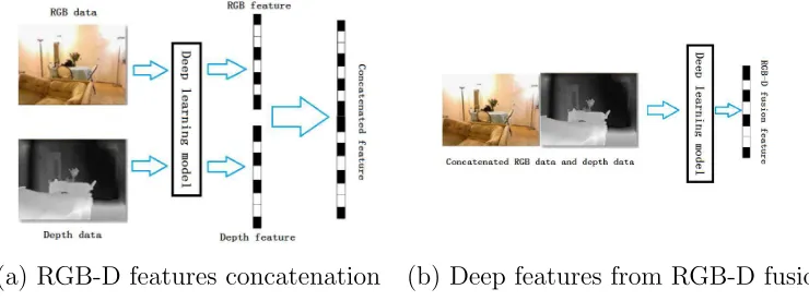
[image:20.612.119.489.414.552.2](a) RGB-D features concatenation (b) Deep features from RGB-D fusion
Figure 6: Illustration about two experimental procedures used in our evaluation work.
4.1. 2D&3D Object Dataset 479
We evaluate deep feature learning for object category recognition on the
480
2D&3D object dataset [12]. This dataset includes 18 different categories (i.e.,
481
binders, books and scissors) with each of them containing 3 to 14 objects
re-482
sulting in 162 objects. The views of each object are recorded every 10 degrees
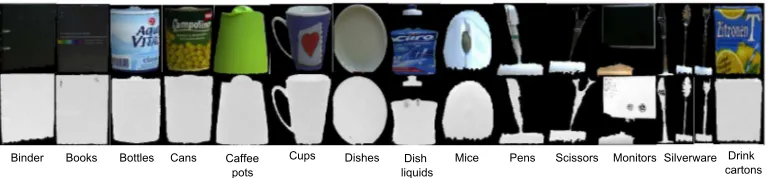
Binder Books Bottles Cans Caffee Cups Dishes Mice Pens Scissors MonitorsSilverware
pots Dish liquids
[image:21.612.115.499.128.217.2]Drink cartons
Figure 7: Example images in the 2D&3D Object dataset, which contains 14 object classes (binder, books, bottles, cans, coffee pots, cups, dishes, dish liquids, mice, pens, scissors, monitors, silverware and drink cartons). There are totally 14 paired samples shown in this figure. The Cropped RGB image is shown on the top and the corresponding depth image is on the bottom.
along the vertical axis. Therefore, there are totally 162×36 = 5832 RGB
484
images and 162×36 = 5832 depth images respectively. For the consistency
485
with the setup in [12], since the low number of examples of classes perforator
486
and phone, our experiments do not include them. Meanwhile, knives, forks
487
and spoons are combined into one category ‘silverware’. Example images
488
from this dataset are given in Fig. 7. We choose 6 objects per category for
489
training, and the left are used for testing. If the number of objects in a
cat-490
egory is less than 6 (e.g., scissors), 2 objects are added into the test. Since
491
images are cropped in different sizes, we resize each image into 56×56 pixels.
492
We give the final comparison results between neural-network classifier and
493
SVM in Table 1.
494
Table 1: The final comparison results between neural-network classifier and SVM on the 2D&3D object dataset. The second, fourth and seventh columns are the results of RGB test images, depth test images and RGB-D fusion test images on the neural-network classifier separately. The third, fifth, sixth and eighth columns are the results of RGB test images, depth test images, concatenated RGB-D image features and RGB-D fusion test images on SVM separately.
Method RGB RGB
(SVM) Depth
Depth (SVM)
RGB-D Concatenation
(SVM)
RGB-D fusion
RGB-D fusion (SVM)
DBNs 72.1 74.5 75.7 78.6 82.3 78.3 79.1
CNNs 77.3 79.1 81.0 83.5 83.6 82.7 84.6
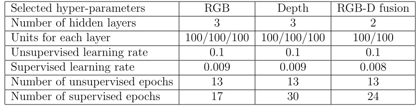
The hyper-parameters of the DBNs, SDAE and CNNs models are
de-495
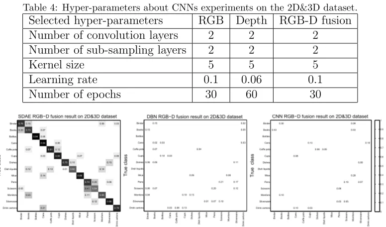
scribed in Table. 2, Table. 3 and Table. 4. Fig. 8 shows confusion matrixes
496
about our three deep learning models across 14 classes on the 2D&3D dataset.
[image:22.612.106.526.226.333.2]497
Table 2: Hyper-parameters about DBNs experiments on the 2D&3D dataset.
Selected hyper-parameters RGB Depth RGB-D fusion
Number of hidden layers 3 3 2
Units for each layer 100/100/100 100/100/100 100/100
Unsupervised learning rate 0.1 0.1 0.1
Supervised learning rate 0.009 0.009 0.008
Number of unsupervised epochs 13 13 13
Number of supervised epochs 17 30 24
498
Table 3: Hyper-parameters about SDAE experiments on the 2D&3D dataset.
Selected hyper-parameters RGB Depth RGB-D fusion
Number of hidden layers 2 2 2
Units for each layer 100/100 100/100 100/200
Unsupervised learning rate 0.1 0.1 0.1
Supervised learning rate 0.1 0.1 0.1
Number of unsupervised epochs 10 10 15
Number of supervised epochs 10 10 30
From the comparison results of our experiments about three selected deep
499
learning models on 2D&3D dataset in Table. 1, it can be seen that the
ac-500
curacy of RGB, depth and RGB-D fusion results through SVM outperforms
501
that through the neural-network classifier. In each deep learning method,
ac-502
curacies of RGB-D concatenation through SVM and RGB-D fusion features
503
through SVM are higher than deep features from RGB data only and deep
504
features from depth data only. In these three methods (DBNs, CNNs and
505
SDAE), CNNs obtain the highest performance (84.6%). From the
compar-506
ison of three confusion matrixes in Fig. 8, we can see that our three deep
507
learning models all have the lowest error rates in bottles, cans, coffee pots
508
and cups. Binders, books, pens and scissors have higher error rates. The
509
main reason is that binders and books are similar in shape and color. Pens,
Table 4: Hyper-parameters about CNNs experiments on the 2D&3D dataset.
Selected hyper-parameters RGB Depth RGB-D fusion
Number of convolution layers 2 2 2
Number of sub-sampling layers 2 2 2
Kernel size 5 5 5
Learning rate 0.1 0.06 0.1
Number of epochs 30 60 30
0.61 0.43 0.30 0.54 0.10 1.00 0.77 0.08 0.10 0.89 0.13 0.92 0.03 0.06 0.92 0.05 1.00 0.72 0.83 0.06 0.03 0.10 0.94 0.05 0.09 0.03 0.28 0.90 0.08 0.07 0.92 0.10 0.87 B in de r B oo ks B ot tle s C an s C of fe p ot s C up s D ish es D ish li qu id s Mi ce P en s S ci sso rs Mo ni to rs S ilve rw are D rin k ca rto ns Tru e cl ass
CNN RGB−D fusion result on 2D&3D dataset
Binder Books Bottles Cans Coffe pots Cups Dishes Dish liquids Mice Pens Scissors Monitors Silverware Drink cartons 0 0.1 0.2 0.3 0.4 0.5 0.6 0.7 0.8 0.9 1 0.83 0.15 0.08 0.06 0.04 0.15 0.80 0.02 0.07 0.05 0.07 1.00 0.03 0.10 0.92 0.03 0.03 0.89 0.06 0.87 0.10 0.13 0.76 0.05 0.13 0.04 1.00 0.87 0.01 0.62 0.20 0.07 0.21 0.55 0.10 0.08 0.73 0.11 0.17 0.12 0.82 0.02 0.05 0.03 0.78 B in de r B oo ks B ot tle s C an s C of fe p ot s C up s D ish es D ish li qu id s Mi ce P en s S ci sso rs Mo ni to rs S ilve rw are D rin k ca rto ns Tru e cl ass
DBN RGB−D fusion result on 2D&3D dataset
Binder Books Bottles Cans Coffe pots Cups Dishes Dish liquids Mice Pens Scissors Monitors Silverware Drink cartons 0.76 0.20 0.05 0.15 0.73 0.07 0.12 0.23 0.94 0.07 0.06 0.94 0.03 0.14 0.21 0.81 0.13 0.06 0.12 0.84 0.75 0.01 0.10 0.60 0.07 0.86 0.74 0.41 0.11 0.20 0.54 0.12 0.06 0.14 0.66 0.15 0.06 0.88 0.03 0.06 0.79 B in de r B oo ks B ot tle s C an s C of fe p ot s C up s D ish es D ish li qu id s Mi ce P en s S ci sso rs Mo ni to rs S ilve rw are D rin k ca rto ns
SDAE RGB−D fusion result on 2D&3D dataset
Tru e cl ass Binder Books Bottles Cans Coffe pots Cups Dishes Dish liquids Mice Pens Scissors Monitors Silverware Drink cartons
Figure 8: Confusion matrixes about three deep learning models on the 2D&3D dataset. The labels on the vertical axis express the true classes and the labels on the horizontal axis denote the predicted classes.
scissors and silverware are similar in shape. It is worth to note that the error
511
rates of binders and books in SDAE and DBNs are much lower than that
512
of binders and books in CNNs, and the error rates of pens and scissors in
513
SDAE and DBNs are much higher than that of pens and scissors in CNNs.
514
The error rates of other categories are approximately similar. This
inter-515
esting phenomenon may be due to the principle of the three different deep
516
learning methods. In addition, it proves that in general SDAE and DBNs
517
are more in common than CNNs.
518
4.2. Object RGB-D Dataset 519
We test these deep learning algorithms on the second dataset called
RGB-520
D object dataset. This dataset contains 41877 images which are organized
521
into 51 categories about 300 everyday objects such as apples, mushrooms and
522
notebooks. All of the objects are segmented from the background through
523
combining color and depth cues. Fig. 9 shows some segmentation objects
524
from this dataset. Every shown object is from one of the 51 object categories.
525
Following the setup in [47], we choose to run category recognition experiments
Figure 9: Some example images in Object RGB-D dataset. We can find 20 paired samples shown in this figure. In each pair, the segmented RGB image is shown on the top and the corresponding depth image is on the bottom.
by randomly selecting one object from the categories for testing. Each image
527
in object RGB-D dataset is resized into 56×56 pixels for consistency with
528
the 2D&3D dataset. Table 5 summarizes the comparison between
neural-529
network classifier and SVM.
530
Table 5: The final comparison results between neural-network classifier and SVM on Object RGB-D dataset. The second, fourth and seventh columns are the results of RGB test images, depth test images and RGB-D fusion test images on the neural-network classifier separately. The third, fifth, sixth and eighth columns are the results of RGB test images, depth test images, concatenated RGB-D image features and RGB-D fusion test images on SVM separately.
Method RGB RGB
(SVM) Depth
Depth (SVM)
RGB-D Concatenation
(SVM)
RGB-D fusion
RGB-D fusion (SVM)
DBNs 80.9 81.6 75.1 78.6 84.3 82.4 83.7
CNNs 82.4 82.5 75.5 78.9 83.4 83.2 84.8
SDAE 81.4 82.0 71.9 73.7 82.3 82.6 84.2
The hyper-parameters of three deep learning models DBNs, SDAE and
531
CNNs are shown in Table 6, Table 7 and Table 8.
532
As we can see from Table 5, CNNs outperform DBNs and SDAE by 0.5%
533
and 0.3%. Due to the limitation of space, we only give the confusion matrix
534
of the best performance (CNNs RGB-D fusion) in our experiments. Fig. 10
[image:24.612.106.529.500.590.2]Table 6: Hyper-parameters about DBNs experiments on Object RGB-D dataset.
Selected hyper-parameters RGB Depth RGB-D fusion
Number of hidden layers 3 3 3
Units for each layer 110/100/20 110/100/20 110/100/20
Unsupervised learning rate 0.1 0.1 0.1
Supervised learning rate 0.009 0.009 0.009
Number of unsupervised epochs 13 13 13
Number of supervised epochs 8 10 22
Table 7: Hyper-parameters about SDAE experiments on Object RGB-D dataset.
Selected hyper-parameters RGB Depth RGB-D fusion
Number of hidden layers 2 2 2
Units for each layer 100/100 130/100 110/200
Unsupervised learning rate 0.1 0.1 0.1
Supervised learning rate 0.1 0.08 0.05
Number of unsupervised epochs 10 15 15
Number of supervised epochs 15 30 30
shows the confusion matrix about CNNs across 51 classes over object RGB-D
536
dataset.
537
4.3. NYU Depth v1 538
Besides image object classification, we also evaluate these three deep
fea-539
ture learning models on indoor scene classification. NYU Depth v1 dataset
540
consists of 7 different kinds of scene classes totally containing 2347 labeled
541
frames. Since the standard classification protocol removes scene ‘cafe’ from
542
Table 8: Hyper-parameters about CNNs experiments on Object RGB-D dataset.
Selected hyper-parameters RGB Depth RGB-D fusion
Number of convolution layers 2 2 2
Number of sub-sampling layers 2 2 2
Kernel size 5 5 5
Learning rate 0.1 0.06 0.03
Bathroom Bedroom Bookstore Kitchen Living room Office
Figure 11: Some example images in the NYU Depth v1 dataset. It includes 6 object classes (bathroom, bedroom, bookstore, kitchen, living room and office). We can find 6 paired samples shown in this figure. In each pair, the segmented RGB image is shown on the top and the corresponding depth image is on the bottom.
the dataset, we use the remaining 6 different scenes. Example images in the
543
NYU Depth v1 dataset are shown in Fig. 11. It is worth noting that since
544
there are so many objects in one scene and the correlation between images
545
in one scene is low, it makes NYU Depth v1 a very challenging dataset.
546
The baseline when only using RGB images is 55% [74]. Table 9 shows the
547
performance comparison between neural-network classifier and SVM on this
548
dataset.
549
Table 9: The performance comparison results between neural-network classifier and SVM on NYU Depth v1 dataset. The second, fourth and seventh columns are the results of RGB test images, depth test images and RGB-D fusion test images on the neural-network classifier separately. The third, fifth, sixth and eighth columns are the results of RGB test images, depth test images, concatenated RGB-D image features and RGB-D fusion test images on SVM separately.
Method RGB RGB
(SVM) Depth
Depth (SVM)
RGB-D Concatenation
(SVM)
RGB-D fusion
RGB-D fusion (SVM)
DBNs 62.4 66.7 57.3 60.8 68.3 65.5 70.5
CNNs 68.4 69.5 56.5 56.9 70.4 70.1 71.8
SDAE 65.2 68.4 51.5 55.0 70.3 69.6 71.1
The hyper-parameters of DBNs, SDAE and CNNs can be found in
Ta-550
ble 10, Table 11 and Table 12. Fig. 12 shows confusion matrixes about our
551
three deep learning models across 6 classes over NYU Depth v1 dataset.
552
As we have mentioned above, NYU depth v1 dataset is very
[image:27.612.110.526.509.600.2]Table 10: Hyper-parameters about DBNs experiments on NYU Depth v1 dataset.
Selected hyper-parameters RGB Depth RGB-D fusion
Number of hidden layers 3 3 3
Units for each layer 120/100/80 120/100/80 110/100/100
Unsupervised learning rate 0.06 0.04 0.1
Supervised learning rate 0.006 0.008 0.008
Number of unsupervised epochs 3 3 3
[image:28.612.115.511.305.411.2]Number of supervised epochs 35 45 22
Table 11: Hyper-parameters about SDAE experiments on NYU Depth v1 dataset.
Selected hyper-parameters RGB Depth RGB-D fusion
Number of hidden layers 3 3 3
Units for each layer 120/100/80 120/100/60 130/200/120
Unsupervised learning rate 0.01 0.01 0.01
Supervised learning rate 0.1 0.1 0.1
Number of unsupervised epochs 15 15 15
Number of supervised epochs 30 35 50
ing. Therefore, in our three deep learning methods, CNNs achieve the best
554
performance which is only 71.8%. Different from 2D&3D object dataset
555
and object RGB-D dataset, RGB-D fusion through SVM always obtains the
556
higher recognition accuracy (70.5% DBNs, 71.8% CNNs and 71.1% SDAE)
557
compared to RGB-D concatenation (SVM) and RGB-D fusion. It may be
558
because the scene images from NYU depth v1 dataset contain many irregular
559
objects which seem much more complicated than the object images from the
560
Table 12: Hyper-parameters about CNNs experiments on NYU Depth v1 dataset.
Selected hyper-parameters RGB Depth RGB-D fusion
Number of convolution layers 2 2 2
Number of sub-sampling layers 2 2 2
Kernel size 8 8 8
Learning rate 0.008 0.008 0.004
0.83 0.11 0.75 0.07 0.08 0.15 0.12 0.72 0.17 0.07 0.71 0.21 0.18 0.75 0.04 0.21 0.10 0.10 0.63 B at hro om B ed ro om B oo kst ore K itch en Li vi ng ro om O ffi ce
CNN RGB−D fusion result on NYU Depth v1 dataset
Tru e cl ass Bathroom Bedroom Bookstore Kitchen Livingroom Office 0 0.1 0.2 0.3 0.4 0.5 0.6 0.7 0.8 0.89 0.04 0.17 0.73 0.04 0.14 0.13 0.70 0.02 0.11 0.13 0.64 0.19 0.10 0.73 0.30 0.15 0.11 0.68 B at hro om B ed ro om B oo kst ore K itch en Li vi ng ro om O ffi ce
DBN RGB−D fusion result on NYU Depth v1 dataset
Tru e cl ass Bathroom Bedroom Bookstore Kitchen Livingroom Office 0.83 0.17 0.74 0.16 0.10 0.74 0.05 0.15 0.17 0.18 0.66 0.08 0.06 0.68 0.06 0.20 0.17 0.11 0.69 B at hro om B ed ro om B oo kst ore K itch en Li vi ng ro om O ffi ce
SDAE RGB−D fusion result on NYU Depth v1 dataset
Tru e cl ass Bathroom Bedroom Bookstore Kitchen Livingroom Office
Figure 12: Confusion matrixes about three deep learning models on NYU Depth v1 dataset. The labels on the vertical axis express the true classes and the labels on the horizontal axis denote the predicted classes.
previous two datasets. From the confusion matrixes about these three deep
561
learning methods, to a great extent, it can be seen that the distribution of
562
error rates is similar.
563
4.4. Sheffield Kinect Gesture (SKIG) Dataset 564
We also evaluate these four deep learning algorithms on video
classifica-565
tion datasets. SKIG is a hand gesture dataset which contains 10 categories
566
of hand gestures with 2160 hand gesture video sequences from six people,
in-567
cluding 1080 RGB sequences and 1080 depth sequences respectively. Fig. 13
568
shows some frames in this dataset. In our experiments, since it has been
569
proved that 5∼7 frames (0.3∼0.5 seconds of video) are enough to have the
570
similar performance with the one obtainable with the entire video sequence
571
[67]. Therefore, each video sequence is resized into 64×48×13. Following
572
the experimental setting in [58], we choose four objects as the training set
573
and test on the remaining data. Table 13 shows the performance comparison
574
between neural-network classifier and SVM on SKIG dataset.
Additional-575
ly, since 3D-CNNs gain much success in video data classification, we use
576
3D-CNNs instead of 2D-CNNs in our experiments. We also compare LSTM
577
Neural Networks experimentally in this subsection.
578
The hyper-parameters of DBNs, SDAE, 3D-CNNs and LSTM can be
579
found in Table 14, Table 15, Table 16 and Table 17.
580
To get better results in the 3D-CNNs model, we decay the learning rate
581
a half in each epoch.
582
Fig. 14 shows confusion matrixes about our four deep learning models
583
across 10 classes on the SKIG dataset.
[image:29.612.113.505.124.239.2]Circle Triangle Turn Pat around Comehere
Cross Z
[image:30.612.114.497.126.229.2]Wave Right-left Up-down
Figure 13: Example frames from Sheffield Kinect gesture dataset and the descriptions of 10 different categories: circle (clockwise), triangle (anti-clockwise), up and down, right and left, wave, hand signal “Z”, cross, comehere, turn around and pat. In each pair, the segmented RGB image is shown on the top and the corresponding depth image is on the bottom.
From the comparison of these four deep learning models in Table 13, we
585
can see that 3D-CNNs achieve the best performance among four - 93.3%.
586
It may be because that 3D-CNNs consider the more temporal correlation
587
between video frames [39]. Sequence learning method LSTM with raw pixel
588
features achieves 91.3% on the SKIG dataset, which is better than the
perfor-589
mances of DBN and SDAE. It is reasonable because LSTM can learn from
590
experience to classify, process and predict time series. Overall, we obtain
591
high accuracies in this dataset. The main reason is that the ten categories in
592
SKIG dataset can be classified easily. Each category is much different from
593
other categories, and every test video in one category is similar to other test
594
videos in the same category. Therefore, in terms of SKIG dataset, inter-class
595
distance is big and intra-class distance is small. The analysis above
sug-596
gests that deep learning will produce a good performance with less training
597
samples if the experimental dataset is not challenging.
598
4.5. MSRDailyActivity3D Dataset 599
The last dataset which we test on is MSRDailyActivity3D dataset [90].
600
It is a daily activity dataset which contains 16 activity types (e.g., drink, eat,
601
play game). There are 10 subjects with each of them performs each activity
602
twice, once in standing position, and once in sitting position. Examples of
603
RGB images, raw depth images in this dataset are illustrated in Fig. 15. We
604
do the same preprocessing procedure like SKIG and resize each sequence to
605
64×48×13. Then subject 1 to subject 5 of “sitting on sofa” and subject 1 to
606
subject 5 of “standing” in this dataset are used as training set and the rest
0.94 0.12 0.18 0.94 1.00 0.06 1.00 0.94 0.06 0.06 0.88 0.06 0.06 0.94 1.00 0.06 0.82 0.06 0.82 C ircl e Tri an gl e U p− do w n R ig ht −l ef t W
ave "Z"
C ro ss C ome he re Tu re a ro un d P at
3D−CNN RGB−D fusion result on SKIG dataset
Tru e cl ass Circle Triangle Up−down Right−left Wave "Z" Cross Comehere Ture around Pat 0 0.1 0.2 0.3 0.4 0.5 0.6 0.7 0.8 0.9 1 0.88 0.12 0.24 0.82 1.00 0.06 0.88 0.06 0.12 0.06 0.88 0.18 0.06 0.88 0.12 0.12 0.76 1.00 0.76 0.06 0.94 C ircl e Tri an gl e U p− do w n R ig ht −l ef t W
ave "Z"
C ro ss C ome he re Tu re a ro un d P at
DBN RGB−D fusion result on SKIG dataset
Tru e cl ass Circle Triangle Up−down Right−left Wave "Z" Cross Comehere Ture around Pat 0.82 0.12 0.24 0.12 0.76 0.06 1.00 0.06 0.06 0.12 0.88 0.12 0.06 0.88 0.06 0.12 0.12 0.76 0.06 0.18 0.76 0.94 0.12 0.64 0.12 0.12 0.76 C ircl e Tri an gl e U p− do w n R ig ht −l ef t W
ave "Z"
C ro ss C ome he re Tu re a ro un d P at
SDAE RGB−D fusion result on SKIG dataset
Tru e cl ass Circle Triangle Up−down Right−left Wave "Z" Cross Comehere Ture around Pat 0.94 0.12 0.18 0.94 1.00 0.06 1.00 0.94 0.06 0.06 0.88 0.06 0.06 0.94 1.00 0.06 0.82 0.06 0.82 C ircl e Tri an gl e U p− do w n R ig ht −l ef t W
ave "Z"
C ro ss C ome he re Tu re a ro un d P at
3D−CNN RGB−D fusion result on SKIG dataset
Tru e cl ass Circle Triangle Up−down Right−left Wave "Z" Cross Comehere Ture around Pat 0 0.1 0.2 0.3 0.4 0.5 0.6 0.7 0.8 0.9 1 0.88 0.12 0.24 0.82 1.00 0.06 0.88 0.06 0.12 0.06 0.88 0.18 0.06 0.88 0.12 0.12 0.76 1.00 0.76 0.06 0.94 C ircl e Tri an gl e U p− do w n R ig ht −l ef t W
ave "Z"
C ro ss C ome he re Tu re a ro un d P at
DBN RGB−D fusion result on SKIG dataset
Tru e cl ass Circle Triangle Up−down Right−left Wave "Z" Cross Comehere Ture around Pat 0.82 0.12 0.24 0.12 0.76 0.06 1.00 0.06 0.06 0.12 0.88 0.12 0.06 0.88 0.06 0.12 0.12 0.76 0.06 0.18 0.76 0.94 0.12 0.64 0.12 0.12 0.76 C ircl e Tri an gl e U p− do w n R ig ht −l ef t W
ave "Z"
C ro ss C ome he re Tu re a ro un d P at
SDAE RGB−D fusion result on SKIG dataset
Tru e cl ass Circle Triangle Up−down Right−left Wave "Z" Cross Comehere Ture around Pat
(a) SDAE (b) 3DCNN
0.94 0.12 0.18 0.94 1.00 0.06 1.00 0.94 0.06 0.06 0.88 0.06 0.06 0.94 1.00 0.06 0.82 0.06 0.82 C ircl e Tri an gl e U p− do w n R ig ht −l ef t W
ave "Z"
C ro ss C ome he re Tu re a ro un d P at
3D−CNN RGB−D fusion result on SKIG dataset
Tru e cl ass Circle Triangle Up−down Right−left Wave "Z" Cross Comehere Ture around Pat 0 0.1 0.2 0.3 0.4 0.5 0.6 0.7 0.8 0.9 1 0.88 0.12 0.24 0.82 1.00 0.06 0.88 0.06 0.12 0.06 0.88 0.18 0.06 0.88 0.12 0.12 0.76 1.00 0.76 0.06 0.94 C ircl e Tri an gl e U p− do w n R ig ht −l ef t W
ave "Z"
C ro ss C ome he re Tu re a ro un d P at
DBN RGB−D fusion result on SKIG dataset
Tru e cl ass Circle Triangle Up−down Right−left Wave "Z" Cross Comehere Ture around Pat 0.82 0.12 0.24 0.12 0.76 0.06 1.00 0.06 0.06 0.12 0.88 0.12 0.06 0.88 0.06 0.12 0.12 0.76 0.06 0.18 0.76 0.94 0.12 0.64 0.12 0.12 0.76 C ircl e Tri an gl e U p− do w n R ig ht −l ef t W
ave "Z"
C ro ss C ome he re Tu re a ro un d P at
SDAE RGB−D fusion result on SKIG dataset
Tru e cl ass Circle Triangle Up−down Right−left Wave "Z" Cross Comehere Ture around Pat 0.88 0.12 0.12 0.12 0.88 1.00 0.06 0.06 0.88 0.12 0.06 0.94 0.06 0.06 0.88 0.12 0.06 0.76 0.94 0.12 0.76 0.12 0.12 0.76 Circle
Triangle Up-down Right-left
Wave
"Z"
Cross
Comehere Turn around
Pat
LSTM RGB-D fusion result on SKIG dataset
True class Circle Triangle Up-down Right-left Wave "Z" Cross Comehere Turn around Pat 0 0.1 0.2 0.3 0.4 0.5 0.6 0.7 0.8 0.9 1
[image:31.612.122.487.194.542.2](d) DBN (e) LSTM