Accepted Manuscript
A parallel Volume of Fluid-Lagrangian Parcel Tracking coupling
procedure for diesel spray modelling
H. Yu , L. Goldsworthy , M. Ghiji , P.A. Brandner , V. Garaniya
PII:
S0045-7930(17)30108-1
DOI:
10.1016/j.compfluid.2017.03.027
Reference:
CAF 3438
To appear in:
Computers and Fluids
Received date:
23 November 2016
Revised date:
24 March 2017
Accepted date:
29 March 2017
Please cite this article as: H. Yu , L. Goldsworthy , M. Ghiji , P.A. Brandner , V. Garaniya , A parallel
Volume of Fluid-Lagrangian Parcel Tracking coupling procedure for diesel spray modelling,
Computers
and Fluids
(2017), doi:
10.1016/j.compfluid.2017.03.027
ACCEPTED MANUSCRIPT
A parallel Volume of Fluid-Lagrangian Parcel Tracking coupling
procedure for diesel spray modelling
H. Yu*, L. Goldsworthy, M. Ghiji, P.A. Brandner, V. Garaniya
Australian Maritime College, University of Tasmania, Launceston, Tasmania 7250
Abstract
A parallel computing Eulerian/Lagrangian multi-scale coupling procedure for diesel
spray simulation is presented. Early breakup of the diesel jet is captured by using a
compressible Volume of Fluid (VOF) method. In regions where the phase interface can no
longer be sufficiently resolved, separated and small scale liquid structures are described by a
Lagrangian Parcel Tracking (LPT) approach, in conjunction with secondary breakup
modelling and a turbulence stochastic dispersion model. The coupling of these two
descriptions utilises a Region Coupling Method and an efficiently parallelised droplet
identification and extraction procedure. This approach enables run-time VOF-LPT field
coupling and filters small-scale liquid structures that are suitable candidates for
Eulerian-liquid-structure/Lagrangian droplet conversion, preserving their position, mass and
momentum. The coupling procedure is initially applied to model the atomisation of a simple
liquid jet and the results are compared with that of a statistical coupling approach to
demonstrate the performance of the developed coupling procedure. Its application is then
extended to simulate a real diesel spray from a nozzle with a sharp entrance. Coupling
in-nozzle phenomena such as flow separation, flow detachment and turbulence to the primary
and secondary spray atomisation, provides a tool for the prediction of complex spray
dynamics.
Keywords: Eulerian (Volume of Fluid); Lagrangian (Lagrangian Parcel Tracking); Parallel
ACCEPTED MANUSCRIPT
ABBREVIATIONS
VOF Volume of Fluid
LPT Lagrangian Parcel Tracking
LES Large Eddy simulation
LSM Level Set Method
DCA Direct Coupling Approach
RCM Region Coupling Method
DIP Droplet Identification Procedure
DEP Droplet Extraction Procedure
SCA Statistical Coupling Approach
ASOI After Start of Injection
NOMENCLATURE
Mixture densityU Velocity
P
Pressuret
Time
Shear stress
Surface tension coefficientl
Liquid volume fractionn
Unit vector normal to the liquid surface Liquid surface curvature
Dirac functionl
Density of the liquid phaseg
ACCEPTED MANUSCRIPT
0
Reference density for the liquid phasel
Compressibility of the liquid phaseg
Compressibility of the gas phase
Mixture dynamic viscosityl
Liquid phase dynamic viscosityg
Gas phase dynamic viscositysgs
Sub-grid shear stressk Sub grid kinetic energy
Kinetic viscositysgs
Sub-grid kinetic viscosity
Turbulent dissipationh Enthalpy
sgs
h
Sub-grid enthalpyp
X
Parcel position vectorp
U
Parcel velocity vectorg
U
Gas phase velocity vectorrel
U
Relative velocity between parcel and gasD
C
Drag coefficientRe
p Parcel Reynolds numberC Cavitation number
ACCEPTED MANUSCRIPT
p
d
Parcel diameterp
Parcel characteristic times U
S Parcel momentum source term
Thermal diffusionZ
Mixture fractionD
Mass diffusionT
TemperatureZ sgs
Sub-grid species mass flux
p
m
Mass of a parcelcell
V
Volume of a mesh cellp
V
Volume of a parcelp
R
Radius of a parcelP
X
Position vector of a parcelcell
ACCEPTED MANUSCRIPT
1.
INTRODUCTION
Achieving an efficient combustion process in diesel engines requires optimally
combined effects of air and fuel mixing, turbulence generation and interaction of spray and
engine geometry. This involves improving the atomisation of the diesel spray by taking into
account various operating conditions such as different nozzle designs, operating temperatures
as well as the injection and chamber pressures. Many studies have focused on these aspects in
an effort to realise more efficient combustion and reduced emissions [1].
In diesel engines, the fuel is injected at a high pressure into the combustion chamber
where it follows a series of disintegration processes. Initially, the interaction between the fuel
and nozzle geometry results in a flow regime dominated by separation, cavitation and
aerodynamic instabilities causing primary jet break-up in the vicinity of the nozzle exit [1, 2].
In this process, the fragmentation of the intact liquid core generates large liquid structures
that will undergo secondary breakup and further disintegrate into small droplets. At the next
stage, the spacing between droplets increases further downstream of the nozzle due to air
entrainment and turbulent droplet-gas interaction, and the droplet size decreases owing to
secondary breakup and evaporation.
The primary and secondary breakup mechanisms have been extensively studied
experimentally, see for example [3-7]. The use of different measuring techniques especially
X-ray analysis of diesel sprays has provided comprehensive information on the liquid
penetration, cross-sectional projected density distribution. The measurement of these
parameters can help gain a qualitative understanding about the diesel spray evolution.
However, the shot to shot variation of sprays makes it difficult to quantitatively capture the
detailed features of the spray at different stages [4]. Therefore, to obtain information on the
spatial and temporal spray evolution with high resolution, computational simulations are
ACCEPTED MANUSCRIPT
Due to the complex behaviour of the diesel spray in the primary and secondary
atomisation processes, various computational approaches have been proposed and developed
to simulate these. For primary atomisation, interface capturing/tracking methods such as the
Volume of Fluid (VOF) method [8-14], Level Set Method (LSM) [15, 16] and the
combination of both[17, 18] are widely adopted. In the VOF method, the liquid and gas are
treated as two immiscible phases that are both described in the Eulerian framework. A
transport equation calculating the volume fraction of each phase in a cell is employed and the
derived gradient of the volume fraction of the dense phase is used to construct the liquid
interface. This intrinsically allows the simulation of jet breakup, liquid core disintegration
and droplet coalescence in a volume conservative manner. However, sufficiently discretising
all small scale liquid structures can lead to exponential increase in mesh elements, leading to
excessive demand in computational time for complex two-phase flow cases. In the secondary
atomisation, due to the increasingly dominant effect of surface tension on small scales, small
liquid structures start to become either spherical or elliptical, and they fall in the framework
of LPT. However, in order for these small structures to be valid for Lagrangian modelling,
they need to be smaller than the grid size. To ensure numerical stability, the maximum size of
particles is recommended to be smaller than 20% of the local grid size for Lagrangian particle
tracking [19, 20]. This is one of the main limitations of the Lagrangian modelling that grid
size could be larger than what might be desirable for good resolution of small scale flow
features. A wide range of Lagrangian models have been developed specifically for the
modelling of spray atomisation. Most of these are based on the Lagrangian description of
individual droplets or parcels with an additional level of modelling for the primary and
secondary atomisation [21-30]. The comparison of four different atomisation models, namely
the Wave model [31], the Huh and Gosman atomisation model [32] and the MPI-1 and MPI-2
ACCEPTED MANUSCRIPT
detailed attention to the effects of in nozzle flow phenomena (e.g. flow separation, cavitation
and turbulence), resulting in the inaccurate prediction of primary spray breakup. However,
they possess the advantage that it is rather efficient to simulate the evolution of a cluster of
small-scale liquid structures without a high demand in computational time. This is enabled by
the use of many well-developed secondary breakup models. Typically, the KH model by
Reitz [23] as one of the earliest developed droplet breakup models predicts the development
of aerodynamically induced disturbances on the liquid surface employing the
Kelvin-Helmholtz (KH) mechanism. This mechanism relates the radii of parent and child parcels
with the fastest growing wave length on the liquid surface and its corresponding growth rate.
The RT model by Amsden et al. [34], on the other hand, describes Rayleigh-Taylor
instabilities growing on a liquid-gas interface due to the density jump between gas and liquid.
A parameter known as the break up time is introduced in this model, and it acts as a trigger to
initiate the breakup process when the growing time of RT waves on the droplet surface is
greater than the break up time. A hybrid model combining the KH and RT models is then
developed to account for both the primary and secondary breakup of jets using a switching
threshold Weber Number We = 12 [35].
In the light of the development of various primary and secondary atomisation
modelling approaches, many attempts have been made to combine the merits of interface
tracking/capturing and Lagrangian particle tracking. One of the first Interface-Tracking/Point
Particle Tracking coupling procedures for jet breakup simulation is reported by Hermann et
al. [36]. A dual grid method in which Eulerian (Level Set) and Lagrangian (point particle
tracking) descriptions of liquid spray are handled respectively on two individual grids with
two-way momentum coupling was first introduced in spray modelling. A similar approach
however with adaptive mesh refinement capability is demonstrated by Tomar et al. [37]
ACCEPTED MANUSCRIPT
droplets are tracked as Lagrangian spherical particles in the region where the mesh is
sufficiently coarse. Both approaches identify liquid structures having a volume smaller than a
predefined threshold value from the Eulerian simulation and transfer them into individual
particles eligible for particle tracking. These methods are often referred to as the Direct
Coupling Approach (DCA) and provide unique ways to deal with mesh inconsistency
problems encountered in simultaneous modelling of primary and secondary spray atomisation.
One of the main drawbacks of DCA is the limitation that droplets generated from Eulerian
simulation can only be expensively tracked as individual particles due to the absence of
secondary breakup modelling. This is either because the exclusive use of velocity field
information in the Eulerian-Lagrangian coupling disables the use of a secondary breakup
model [36] or the computational power is insufficient for the integration of an adaptive mesh
refinement method with secondary breakup modelling [37]. Consequently, applications of
these approaches are limited to capturing only a small segment of the liquid jet breakup
process (e.g. only 30 µs after start of injection in Hermann et al. [36] and five days for one
unit time in Tomar et al. [37]). On the other hand, the secondary breakup models, typically
the KH-RT model, can group fluid particles of similar properties in a limited number of
parcels. The use of the parcel concept can ease the computational strain by reducing the
number of individual particles tracked in the Lagrangian modelling of the spray. Without the
parcel assumption, the application of the DCA methods to detailed study of complex
multiphase flows is computationally restricted. Alternatively, the development and
implementation of a Eulerian-Lagrangian Spray Atomisation (ELSA) model attributed to
Burluka et al. [38] and Desportes et al. [39] effectively integrated the Lagrangian parcel
tracking with a single phase Eulerian model. However, this model treats liquid and gas as a
single phase mixture, hence the surface tension effect is not accounted for. The evaluation of
ACCEPTED MANUSCRIPT
liquid/gas interface density. More recent developments in spray modelling give rise to many
mathematical approximations that statistically couple the primary and secondary atomisation
processes. A representative study conducted by Grosshans et al. [40] presents the use of a
coupling layer located within the region where the transition from primary to secondary
atomisation occurs. The volume, velocity and position of liquid structures are sampled on the
coupling layer in the Eulerian frame work till statistical convergence is achieved. Sampled
data are then implemented as initial conditions with the parcel assumption for the subsequent
modelling of secondary atomisation in a Lagrangian reference. In contrast, the probability
density functions of the droplet size were extracted from the entire Eulerian domain by Befrui
et al. [41] and the sampled size distribution data were used to reinitialise the spray simulation
using the Lagrangian parcel tracking method. The statistical coupling procedures are
advantageous in terms of efficiency and have relatively higher accuracy as compared to the
pure Lagrangian description of the liquid spray. However, the stochastic way in which data
are sampled and initialized for the second stage of spray modelling inevitably compromises
the flow information supplied by the more accurate Eulerian modelling of the in-nozzle and
near-nozzle flow. Also, their applications are limited to modelling static sprays due to the fact
that the primary and secondary sprays are not directly coupled.
The objective of this study is therefore to advance the recent work on
Eulerian/Lagrangian coupling [10, 36, 40, 41], using an open source finite volume tool
OpenFOAM, by (1) development of a parallel processing procedure for the identification and
extraction of droplets from VOF simulation and injecting them in the LPT framework, (2)
development of a conservative transient region coupling procedure that allows runtime
exchange of fluid information between VOF and LPT in the region where
Eulerian-Lagrangian transition occurs, (3) integration of a sub-grid stochastic turbulent droplet
ACCEPTED MANUSCRIPT
and (4) allowing the modelling of the secondary breakup of large droplets extracted from the
VOF simulation and the generation and tracking of child parcels in the LPT simulation. The
developed code enables simulation for the complete evolution of the transient diesel spray
from in-nozzle flow to atomised droplets.
2.
NUMERICAL METHODS
2.1. Region Coupling Method
One of the most challenging problems in diesel spray simulation is the different scales
with which the continuous phase and the dispersed phase are modelled. Specifically, the
primary breakup of the liquid jet requires a refined grid to capture the surface instabilities
which generate large ligaments. These ligaments further interact with surrounding gases to
produce smaller liquid structures (droplets) which are rather expensive to be discretised by an
even finer grid. They fall in the Lagrangian reference that entails a coarse grid typically 5
times the size of droplets [19, 20]. This mesh inconsistency problem has been tackled either
by a dual grid approach [10, 36] or a statistical coupling [40, 41] with the former being more
accurate and the latter being more computationally efficient. The dual grid approach uses two
entirely overlapping grids of different resolution, between which the exchange of momentum
is performed with a conservative interpolation scheme [16]. However, due to the discrepancy
in resolution between the two grids, the loss of background flow information is inevitable in
the interpolation process. This problem is more severe in most statistical coupling approaches,
which utilise statistically converged data sampled from the Eulerian simulation to initialise
the Lagrangian simulation. The Region Coupling Method (RCM) described in this section
overcomes the problems of both approaches.
The RCM employs two grids that are only partially overlapping. It enables regional
coupling of an Eulerian liquid-Eulerian gas (VOF) regime with an Eulerian gas-Lagrangian
ACCEPTED MANUSCRIPT
the liquid-gas mixture in the VOF simulation and the carrier phase (gas) in the LPT
simulation. After receiving field information from the VOF simulation, the two-way
interaction of the carrier phase and droplets is handled in the LPT simulation. The effects of
the droplet dynamics on the carrier phase is then reflected on the VOF simulation through the
two-way field interpolation process. The overlapping region is where the transition from
primary to secondary spray atomisation occurs and it couples the VOF and LPT simulations
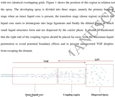
with two identical overlapping grids. Figure 1 shows the position of this region in relation to
the spray. The developing spray is divided into three stages, namely the primary breakup
stage when an intact liquid core is present, the transition stage (dense region) at which the
liquid core starts to disintegrate into large ligaments and finally the diluted phase in which
small liquid structures form and are dispersed by the carrier phase. It should be mentioned
that the right end of the coupling region should be placed far away from the maximum liquid
penetration to avoid potential boundary effects and to prevent unconverted VOF droplets
[image:12.595.45.426.236.558.2]from escaping the domain.
Figure 1: Region VOF-LPT coupling for a liquid diesel spray. The RCM is employed in the coupling region where VOF and LPT overlap.
One disadvantage of the RCM is that a decision has to be made as to where to place
the overlap region, which requires that the Eulerian code needs to first be run till the liquid
penetration reaches maximum within a predefined injection period. The maximum liquid
VOF LPT
ACCEPTED MANUSCRIPT
penetration is defined at the furthest point (along the penetration) where a grid cell has a
liquid volume fraction (
l ) greater than 0.05.However, a relatively coarse mesh can be employed with the VOF method to estimate
the maximum liquid penetration. Alternatively, the use of generic experimental data can also
help determine the extent of a diesel spray by using the Musculus and Kattke model [42], for
example. The present study utilises an incremental method where the VOF domain is
gradually extended to accommodate the maximum liquid penetration. This is achieved
through expanding the VOF computational domain incrementally along the penetration and
reinitialising the simulation with the new domain by mapping the field data from the previous
simulation. In this process, the time and location at which major breakup of the liquid core
occurs are also determined. After the maximum liquid penetration has been estimated, the
coupling region should be placed to encompass the entire dense (major breakup) region that
encompasses most large ligaments. Also, the end of the VOF/coupling region is placed far
away from the maximum penetration to allow flow recirculation and avoid pressure reflection.
The latter is achieved by employing a non-reflective boundary condition at the end of the
VOF domain. The same grid generation strategy is also applied in the direction perpendicular
to the penetration. This prevents all liquid structures from escaping the domain.
In the coupling region, it is computationally difficult to sufficiently describe all liquid
structures of different scales using a refined grid with the VOF method. Therefore, the mesh
resolution is progressively coarsened along the penetration of the liquid jet. The transition
from a fine grid to a relatively coarse grid corresponds to the transition from VOF to LPT.
The transition from VOF to LPT results in the decrease in the number of mesh elements that
can be used to capture the interface of a liquid structure. At some points, the interface of the
generated liquid structures can no longer be sufficiently resolved by the VOF method. These
ACCEPTED MANUSCRIPT
sufficiently smaller than the local cells in which their centroids lie. Therefore, a Droplet
Identification Procedure (DIP) and a Droplet Extraction Procedure (DEP) comparing the
volume of a liquid structure with the volume of a local cell containing this structure‟s
centroid are developed. The code automatically adapts to the grid and frees users from
defining a fixed threshold volume. It allows a greater variety of droplet diameters with a
non-uniform grid than a non-uniform one. However, a threshold percentage determining the amount
by which a liquid structure is smaller than its host cell needs to be defined. In this study, a
liquid structure is recognised as a suitable Lagrangian droplet candidate if it has a volume
smaller than 20% of the host cell‟s volume in the coupling region, as suggested in Arlov et al.
[19].
The droplet conversion procedure enables the use of identical grids for both the VOF
and LPT simulations in the coupling region. It solves the mesh inconsistency problem and
allows high fidelity field coupling between VOF and LPT as the field mapping can be
performed between two identical grids. Since interpolating field information between two
identical grids produces negligible dissipation especially in mapping sub-scale kinetic energy,
this method is independent of the turbulence model used. On the other hand, Large Eddy
Simulation is chosen as the closure model for the governing equations in the present study. It
is a less computationally intensive alternative to Direct Numerical Simulation and offers
better ability to reflect the effects of local turbulence on the evolution of the bulk flow than
the Reynolds averaged governing equations. However, it is only used to demonstrate the
ability of the coupling procedure to model a transient diesel spray. The grid resolution is not
necessarily fine enough for high resolution LES throughout the entire computational domain.
To reduce the computational intensity, the DIP and DEP as well as the two-way field
mapping between VOF and LPT are deployed only in the coupling region. The two-way field
ACCEPTED MANUSCRIPT
utility of OpenFOAM [43], known as cellVolumeWeight. It is a volume averaging algorithm
that allows cell to cell conservative mapping of vector and scalar fields between two grids.
2.2. VOF
The VOF employed in the present study is based on a mathematical model composed
of governing equations for the conservation of mass and momentum of a two-phase system,
accredited to E. De Villiers et al. [44]. This system comprises two immiscible, compressible
fluids and accounts for the surface tension between the two-phases. The single set of mass
and momentum transport equations are:
U
0 t
(1)
'
( )
S t
U
U U p n x x ds
t
(2)where U is the velocity and
is the mixture density. The mixture density
is closelyrelated to the local volume fraction
of each phase with
1 representing acomputational cell fully filled with liquid, while
0 indicates a cell entirely occupied bygas. Any cell having 0
1 contains an interface segregating liquid and gas. For liquid-gascalculations, the mixture density in each computational unit is obtained from:
1
l l l g
(3)where
l is the volume fraction of liquid phase,
l and
g are the respective liquid and gasdensities.
The integral term in equation (2) is a Dirac function that only produces a non-zero
value when '
xx which is an indication of the existence of a liquid interface. This source
term accounts for the effect of surface tension force on the liquid jet breakup process. The
evaluation of this term is achieved following E. De Villiers et al. [44] through the continuum
ACCEPTED MANUSCRIPT
'
( ) S t
n x x ds
(4)where
is the surface tension coefficient,
is the volume fraction of the liquid phasewhich is obtained from the solution of a transport equation:
U
0 t
(5)
and n is a unit vector normal to the liquid surface, is the interface curvature calculated
from the solution of liquid phase volume fraction
:
(6)The system of equations is closed by an equation of state:
0 l l g g
p
p
(7)with
l and
l being the compressibility for liquid and gas phases respectively. Thedynamic viscosity of the mixture is obtained through:
1
l l l g
(8)The VOF interface tracking method is a simple and flexible approach for the
prediction of two-phase flows. A major limitation of this method is its limited ability to
ensure boundedness of liquid volume fraction and preserve sharp interfaces without an
interface reconstruction algorithm such as Piecewise Linear Interface Construction (PLIC)
[46]. In the context of OpenFOAM, this problem is tackled with a „Multi-Dimensional
Universal Limiter with Explicit Solution” (MULES) accredited to Henry Weller together
with the CICSAM interface compression scheme [47]. However, the numerical instabilities
due to unboundedness of liquid volume fraction are not fully eliminated. Alternatively, high
ACCEPTED MANUSCRIPT
Mesh Refinement [37]) or global grid refinement [48]. The present study adopts a globally
refined grid for the VOF simulation. Another limitation of the current compressible VOF
method is that the generated gas at low pressure sites is given the properties of air due to the
lack of a phase change model. The generation of gas is primarily due to the flow separation
downstream of the sharp nozzle inlet. The flow separation causes detachment of liquid from
the wall and gas has to be introduced to satisfy the unity volume fraction (
l
g
1
) undera two phase flow regime. This gas does not condense back to liquid fuel when the local
pressure recovers above the vapour pressure. The incondensable gas then accumulates along
the wall, causing complete detachment of liquid from the nozzle wall (hydraulic flip).
The LES model is integrated in equations (1), (2) and (4) through a local volume
averaging procedure that decomposes relevant phase-weighted hydrodynamic variables into
resolvable and sub-grid scale components. The elimination of the sub-grid fluctuations from
direct simulation is done through a filtering process together with the non-linear convective
terms in equation (2). This process generates additional terms comprising correlation of
sub-scale variables that entail closure through additional modelling. Of these terms, the most
crucial one is the Sub-Grid-Scale (SGS) stress that governs the effect of unresolved
turbulence scales on momentum transport process and its dissipation. This term is defined as:
sgs U U U U
(9)The closure of the SGS stress is achieved through a sub-grid eddy viscosity model given as
2 3 T sgssgs U U kI
(10)
in which k is the SGS turbulence kinetic energy and
sgs is the SGS turbulent viscosity.These SGS turbulence parameters are calculated by using a one-Equation eddy model for
ACCEPTED MANUSCRIPT
1
: 2
T
sgs sgs
k
kU k U U
t
(11)
where
C k
(3/2)/
is the turbulent dissipation,
sgsC kk (1/2) is the SGS kinematicviscosity (
3V
represents the SGS length scale in which V represents the volume of thecomputational cell under consideration). The turbulent coefficients found from statistical
analyses are
C
k
0.07
andC
1.05
[49]. As the emphasis of this study is placed mainlyon obtaining reasonable resolution of spray simulation and the current implementation of
LES is sufficient for this purpose, other SGS terms pertaining to density, mass transfer, phase
fraction and surface tension are neglected.
2.3. LPT
The LPT method is derived based on the consideration of momentum exchange
between the gas phase and the dispersed liquid phase, which is primarily described in the
work of Jangi et al. [26]. This is achieved through the inclusion of additional source terms for
the exchange rate of mass ( Ss SZs ), momentum (
S
Us ) and heat (S
hs ) between the two phases in the gas phase governing equations, while the dynamics of the liquid phase arehandled by Newton‟s second law. The evaporation of fuel is not considered in the present
study as the spray is modelled at room temperature, therefore Ss and
S
Zs are assumed to be zero. The Favre-filtered LES conservation equations for the gas phase can be expressed as
U
S
s0
t
(12)s sgs U
U
UU
S
t
(13)
ssgs h
h
U h
T
h
S
t
ACCEPTED MANUSCRIPT
Z s0
sgs Z
Z
U Z
D
Z
S
t
(15)The over-line signifies the general filtering
( , )x t G r x( , ) (x r t dr, )
(16)where the integration is applied to the entire field with the filtering function satisfying the
normalization condition
( , ) 1
G r x dr
(17)The tilde represents the Favre filtering
(18)in which is a dependant fluid field variable.
Apart from general fluid parameters, enthalpy h , thermal diffusion coefficient
,mass diffusion coefficient
D
, mixture fractionZ
and SGS species mass fluxes Zsgs can be introduced to account for energy exchange and to ensure conservation. While theone-equation eddy model can be utilised to estimate the SGS stress term
sgs , the additionalterms
h
sgs and Zsgs entail closure in order to close equations (14)-(15). They are modelled using a gradient diffusion-closure:Pr
sgs sgs p sgs
h
C
T
(19)sgs Z
sgs sgs
Z
Sc
(20)In Lagrangian spray simulation, the spray is considered as a discrete phase comprising
a large quantity of parcels that are transported using Newtown‟s second law. The LPT
method then provides closure for the source terms SUs in equation (13). The dynamics
ACCEPTED MANUSCRIPT
P P
d
X U
dt (21)
Re Re
24 24
D P D P
P g P rel
P P
C C
d
U U U U
dt
(22)and the drag coefficient is estimated as:
2/3
24 1
1 Re Re 1000
Re 6
0.424 Re 1000
D P P
P D P C C (23)
Here
X
P is the parcel position vector andU
P is the parcel velocity vector. The relativevelocity
U
rel between the parcel and the surrounding gases is denoted asU
g
U
P. For simplicity, the interaction between liquid and gas phases is accounted for by considering onlythe gravity and drag forces experienced by each parcel. The calculation of this force is given
in equations (23) where the parcel Reynolds number is expressed as ReP
gUrel dP/
gwith
g being the density of gas phase,d
P being the parcel diameter and
g being the gasphase dynamic viscosity.
P
PdP2/18
g is the time taken for a parcel to respond to localdisturbances, also known as the parcel characteristic time. The instantaneous local velocity
difference
U
rel cannot be directly evaluated and requires closure. The current study employsO‟Rourke‟s stochastic turbulence dispersion (STD) model [50] to estimate
U
rel which, inLES formulation, can be written as:
'
rel P p
U U U U (24)
where U can be obtained by solving equation (13) and '
P
U is the stochastic velocity vector
accounting for the localised dispersion of parcels through the interaction with gases. UP' is
ACCEPTED MANUSCRIPT
zero. In this way, the Gaussian distribution '
'
2, ,
( P i) 1/ 2 exp P i/ 2
G U U randomly
assigns values to each component of '
P
U at every integration step of the gas (Eulerian) phase.
In each computational cell, the momentum source term in equation (14) can be then obtained
from:
,
1
s
U p P i
cell d
S m U
V dt
(25)in which
m
p is the mass of parcels under consideration and the summation is over all parcelsexisting in a computational cell having a volume of
V
cell.2.4. Secondary breakup model
According to Solsjö et al. [51], it is reasonable to assume that Kelvin-Helmholtz (KH)
and Rayleigh-Taylor (RT) instabilities can occur simultaneously in the secondary breakup
regime due to the high injection velocity. The KH-RT breakup model is therefore utilised to
predict the atomisation process of secondary droplets in the LPT-LES simulation. In the
present study, the KH-RT model allows the generation of parcels from the breakup of the
large Lagrangian droplets (parent droplets) converted from the VOF liquid structures.
Specifically, the diameters of the generated parcels (which are also referred to as child
parcels) are determined by the KH-RT model after the breakup of the parent droplets. The
number of fluid particles a child parcel contains is then determined by ensuring mass
conservation before and after the secondary breakup of a parent droplet. Further details of the
implementation of the KH-RT breakup model as well as the model
constants (
B
0
0.61,
B
1
10,
C
RT
0.1,
C
1
) used in this study can be found in Kitaguchi etACCEPTED MANUSCRIPT
2.5. Collision model
The collision of parcels is handled by a Stochastic Trajectory Collision (STC) model
[53]. Unlike the O‟Rourke collision model [54] which initiates collision of two parcels when
they occupy the same computational cell and their estimated probability of collision is higher
than a threshold value, the STC model takes the trajectory of each participant into account.
This model considers the onset of collision between two parcels when their trajectories
intersect, and the intersection point is reached at the same time within one Eulerian
integration step.
2.6. Droplet Identification Procedure (DIP)
In this section, the development of a parallel droplet identification procedure is
described. This procedure is designed to identify liquid structures that are smaller than 20%
of their host cell‟s volume. In addition, it is determined that these liquid structures should be
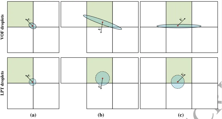
discretised by less than 5 mesh cells in order to minimise the effect of droplet eccentricity.
Specifically, in the case that a small liquid structure satisfies the maximum volume criterion
for VOF-LPT conversion and is spread over 5 or more mesh elements, it can have rather high
eccentricity as depicted in Figure 2. Extracting such a liquid ligament and representing it with
a spherical droplet in the LPT simulation can be a significant source of error especially for
sub-grid physics. Therefore, only liquid structures that satisfy the minimum volume
requirement and are discretised by less than 5 elements are considered eligible candidates for
VOF-LPT conversion. Further, only identifying and extracting liquid structures occupying
less than 5 mesh elements is computationally advantageous that such a process is not
ACCEPTED MANUSCRIPT
Figure 2: Three moving liquid structures having a velocity vector U and a volume smaller than 20% of their host cell (shaded in green) are captured by 4 mesh cells (a), 5 mesh cells (b) and 6 mesh cells (c) in the VOF domain. After a volume conservative conversion to LPT droplets, they are represented with spherical droplets at the same location in the LPT domain.
In the context of OpenFOAM, field values such as velocity, pressure, temperature and
liquid volume fraction (
l ) are stored at the centre of the controlled volumes (mesh cells).The interpolation of the cell-centred values to the face centres based on the face flux
(advection) and values in neighbouring cells is fundamental to the finite volume method. The
interpolation methods and schemes are detailed in Rusche [55]. In the present study, the
identification process involves grouping adjacent liquid-containing cells (
l0.05
) sharingone cell face which has a liquid volume fraction
l0.05
to form contiguous liquidstructures. The reason for the selection of
l
0.05
is to minimise the numerical instabilitiesintroduced by the unboundedness of liquid volume fraction in each computational cell. The
unboundedness of liquid volume fraction means that a cell with
l
0
could have a
lfluctuating between 0 and 10-6 depending on the solver‟s precision. For mesh cells with
relative poor orthogonal quality, the range of fluctuation can become larger (10-3) depending
on the temporal resolution and number of corrections in the MULES loop. The use of a
(a) (b) (c)
V
OF
d
ro
p
le
ts
L
PT
d
ro
p
le
[image:23.595.50.428.99.303.2]ACCEPTED MANUSCRIPT
smaller liquid volume threshold can result in the generation of a large number of physically
unrealistic small droplets mainly due to oscillation of liquid volume fraction. This does not
ensure mass conservation in the VOF-LPT conversion process. On the other hand, using a
larger threshold can lead to the negligence of a considerable amount of small liquid structures
that have a volume fraction slightly higher than 0.05. Allowing these droplets to be
continuously modelled by the VOF method constitutes a significant source of error for the
modelling of sub-grid physics in the VOF simulation. Moreover, the identification method is
slower with the use of a smaller threshold liquid volume fraction. Typically, using
l0
canresult in the increase in computational time by an order of magnitude compared to that of
0.05
l
.In the developed procedure, the identified contiguous structures‟ velocities (
U
P ),centroids (
x
P ) and equivalent spherical diameters (R
p ) are evaluated as:p l cell N
V
V (26)1 3 6 1 2 P p V R
(27)
1
P cell l cell N
P
X X V
V
(28)1
P l l cell N P
U U V
V
(29)HereafterNis the total number of adjacent computational cells with a liquid volume fraction
greater than 0.05. The summation is over all identified mesh cells that belong to a complete
liquid structure. The identification process is shown in Figure 3(a). To ensure the uniqueness
of every liquid structure across the entire domain, the next step is to update the IDs of all
ACCEPTED MANUSCRIPT
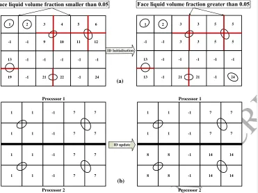
Figure 3: (a) ID initialisation of liquid structures. Adjacent liquid-containing cells sharing a
cell face with
l0.05
(marked in red) are combined to form contiguous liquid structures. The ID of a combined liquid structure is changed to be the same as the associated cell bearing the smallest ID. An individual cell containing liquid but not having a liquid containing neighbour is also identified as an individual liquid structure. Cells of zero liquid volume fraction are tagged with -1. (b) Updating of the liquid structure IDs across the computational domain. Each processor adds the maximum ID received from its higher ranked neighbour to its local liquid structures to ensure the uniqueness of every liquid structure in the domain.2.7. Droplet Extraction Procedure (DEP)
In parallel computing mode, another important point that should be considered is the
preservation of liquid structures that are on or approaching processor patches. This is because
when a liquid structure moves from one processor domain to another, it is possible for it to be
broken into droplets that are then erroneously extracted from the domain by the DEP. This
procedure identifies liquid structures smaller than a pre-defined volume threshold, extracts
and converts them to spherical droplets (by assigning
l
0
to corresponding cells in the1 1 1 1 7 7 7 7 -1 -1 1 1 1 1 7 7 7 7 -1 -1 1 1 1 1 7 7 7 7 -1 -1 8 8 8 8 14 14 14 14 -1 -1 Processor 1 Processor 2 Processor 1 Processor 2 3 4 9 10 5 11 6 12 3 3 3 3 3 5 5 5 5 0 -1 1 2 -1 -1 1 2 -1 -1 15
13 -1 -1 -1 -1 -1
24
19 -1 21 22 -1
15
13 -1 -1 -1 -1 -1
24
13 -1 21 21 -1
(a)
ACCEPTED MANUSCRIPT
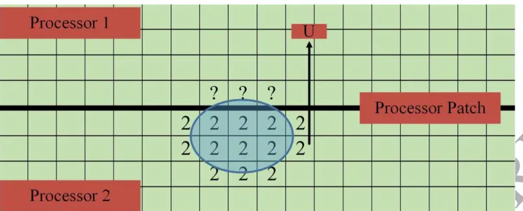
[image:26.595.50.424.146.297.2]VOF domain) that are injected into the Lagrangian domain. This situation is illustrated in
Figure 4.
Figure 4: A liquid structure (ID=2) which is crossing the processor patch with a velocity vectorU. The portion that could be erroneously extracted is tagged with question marks.
When a liquid structure crosses the processor patch, one cell in processor 1 will
experience an increase in liquid volume fraction. Initially, as the liquid content might be too
small to occupy this cell and there are no neighbours with
l
0.05
, the liquid containedwould be recognised by the DEP as a suitable candidate for liquid structure-droplet
conversion if a threshold of one cell volume was defined. Consequently, the entire liquid
structure shown in Figure 4 would be non-physically extracted and transferred into same size
Lagrangian droplets. These droplets could have a volume smaller than or equal to the volume
of the first host cell in processor 1, and the size of computational time step largely governs
the rate at which volume fraction increases in this cell. The degree of this problem is
increasingly noticeable when high temporal resolution is required, especially when running
LES.
A protection procedure is thus developed and implemented to tackle this problem. It
simply stores IDs of all cells that are on processor patches in a Hash-table as different keys.
These “keys” are triggered to locally deactivate the DEP when a liquid structure is detected to
ACCEPTED MANUSCRIPT
that are not on or in close proximity to process patches. One disadvantage of such method is
that it is dependent on the number and location of processor patches. Liquid structures
suitable for VOF-LPT conversion which are in the vicinity of processor patches are not
extracted such that this can be a source of error for the subsequent LPT simulation. However,
contribution of this error can be negligible due to the small number of processor patch cells as
compared to cells in the decomposed domain especially for high level parallel applications.
Finally, properties of all the extracted liquid structures are sent to the master processor by its
slaves and are stored in three Hash-tables (Table 1) designated to record liquid structures‟
(pre-LPT droplets) IDs and their corresponding
x
P ,U
P andR
p .Table 1: Hash-tables storing properties of pre-LPT droplets.
Hash-table 1 Hash-table 2 Hash-table 3 Droplet ID
p
R
Droplet IDX
P Droplet ID pU
11
R
1( , , )
x y z
1 1 1 1( , , )
u v w
1 1 12
2
R
2( , , )
x y z
2 2 2 2( , ,
u v w
2 2 2)
3
3
R
33 3 3
( , , )
x y z
33 3 3
( , ,
u v w
)
…. …. …. …. …. ….
The implementation of the identification and extraction procedure has a limited
influence on the parallel efficiency of the original VOF code in OpenFOAM, simply because
it does not increase the communications between processors as the assembly of liquid
structures is strictly restricted within each processor domain. The use of the protection
procedure eliminates the need to assemble liquid structures across processors, which would
be computationally expensive. The complete droplet identification process is schematically
ACCEPTED MANUSCRIPT
Figure 5: Flow process for parallel droplet identification algorithm.
In the present study, the LPT droplets are not converted back to VOF liquid structures
when the mesh is sufficiently fine for VOF simulation. This decision is made based on
considering the complexity and accuracy of the reversed VOF-LPT transition. Specifically, it
is difficult to determine which and how many cells to which liquid volume fraction would be
assigned to represent one Lagrangian droplet. Also, converting Lagrangian droplets into VOF
ligaments without taking into account how the liquid interface of the ligaments is distributed
across various VOF cells could be a large source of error especially for the modelling of
sub-grid physics. Implementing algorithms to accurately describe the LPT-VOF transition would
require development of a new sub-grid Eulerian model which is beyond the scope of this
study. In addition, executing such a complex algorithm in transient LES simulations could be
impractical because only marginally higher accuracy would be gained at the expense of
greatly increased computing time. Initialise cell IDs
according to their reference in mesh
Find the liquid volume fraction of each cell
Cell(α)
Proceed to next cell
α<0.05
Check If the cell has neighbours with α > 0
Find the smallest cell ID and assign it to the liquid structure it
belongs to
YES
α > 0.05 Check if any of these
adjacent cells are on processor patches
NO
Check if this cell is a processor patch cell
NO
YES
Evaluate Xp, Up and Rp of each complete liquid structure and assign α= 0 to all
relevant cells Store data in
corresponding hash-tables Proceed to next time
step
Update IDs of all liquid structures according to the ranking of their host
processor
YES
NO
Evaluate Vp If Vp < volume
threshold
YES
NO
Initialise cell IDs according to their reference in mesh
ACCEPTED MANUSCRIPT
Before the publication of this work, the capabilities of the developed parallel droplet
identification and extraction procedures have been demonstrated in Ghiji et al.‟s work [56, 57]
(up to 512 CPUs) to be able to quantify the effects of grid resolution on the number of
secondary droplets generated due to the breakup of liquid jet.
2.8. Droplet injector
The next step in VOF-LPT coupling is the injection of droplets transferred by the
DEP to the Lagrangian domain. The injection process must satisfy conservation laws in order
to preserve the accuracy of coupling. This involves developing a utility able to read
information from the three Hash-tables and transform them into Lagrangian droplets,
preserving their mass, momentum and positions. A new automatic injector with such
capabilities is developed as part of the coupling method. This injector scans every entry in the
three Hash-tables at run-time and acquires the volume, position and velocity of the droplets to
be injected. The process diagram shown in Figure 6 schematically depicts how this injector
works.
Figure 6: Process flow for the droplets injection. The customised droplet injector reads information from the Hash-tables and converts it into droplets that are injected into the LPT simulation. Numerical approach
Based on the recent work of Ghiji et al. [57], the governing equations are solved by
OpenFOAM using a Pressure Implicit with Splitting of Operator (PISO) algorithm. In each
Eulerian time-step, the intermediate velocity field ( *
U ) in the VOF simulation is first
Read the droplet position Xp
Check if a cell encompassing this location can be found in
the LPT domain Proceed to next entry in
Hash-table 2
NO
Read the droplet diameter (Rp) from Hash-table 1
YES Evaluate the
droplet volume (Vp)
If Vp > 0 Read the droplet velocity (Up) from
Hash-table 3 Inject
Droplets
YES
NO Proceed to next entry
[image:29.595.46.428.235.566.2]ACCEPTED MANUSCRIPT
evaluated using a semi-discretised momentum equation which consists of a predicted velocity
field, an explicit pressure correction term and a surface tension source term [58]:
* 1
1
( n ) 1
n surface
H U
U p S
a a
(30)
where
U
n1 andp
n1 are velocity and pressure fields mapped from the LPT solution obtainedfrom the previous Eulerian time-step.
Divergence of the predicted velocity field is then substituted into the two-phase
pressure equation of which the detailed derivation can be found in our previous work [59]:
1 1 1 1 * 1 0l n l n
l n l g n g
l g p p U U t t U
(31)Equation (30) is then recalculated to update the velocity field using the solution of equation
(31). The evaluated pressure (
p
n ) and velocity (U
n ) fields are then mapped to the LPTsimulation to initiate a similar pressure-velocity coupling procedure (comprising the particle
force source term
S
particle) within the same Eulerian time-step:* ( n) 1
n particle
H U
U p S
a a
(32)
* 1 0 n n g g p U U t (33)
Finally, the calculated pressure (
p
n1 ) and velocity (U
n1 ) fields are mapped to the VOFsimulation to initiate the next Eulerian time-step.
To solve the pressure-velocity coupling equations, a bounded Normalised Variable
(NV) Gamma differencing scheme [60] with a blending factor of 0.2 is used for the
ACCEPTED MANUSCRIPT
interface capturing. A conservative, second order scheme (Gauss linear corrected) is
employed for Laplacian derivatives and a second order backward discretisation scheme is
adopted for temporal terms.
3.
TEST CASE
A comparison of the RCM and a statistical coupling approach (SCA) is presented in
this section. The test case, as outlined in the work of Grosshans et al.[40], concerns the
atomisation of a simple diesel spray injected from a nozzle which has a diameter (d) of 100
µm. The liquid jet has an initial injection velocity of 500 m/s following a top hat profile at the
nozzle exit, which corresponds to a Reynolds number of 15000 and a jet Weber number of
1.2 × 10⁶. The ambient is filled with air of which the density is 14.8 kg/m3. The ambient
pressure is 52 bar and the liquid and gas have a density ratio of 10 and a viscosity ratio of 46.
3.1. Comparison of VOF simulation
Similar to Grosshans et al.‟s statistical coupling approach, a VOF simulation is first
run to determine the position of the coupling region. In this case, the coupling region is
placed where the averaged liquid volume fraction along the centre line of the jet is lower than
0.25 indicating the onset of major jet breakup. The liquid volume fraction is averaged at
every time-step using OpenFOAM‟s runtime field-Averaging utility and the averaging time
relates to the jet crossing the domain 15 times. A Cartesian equidistant grid duplicating the
highest resolution case (cell size = 0.05d) considered in Grosshans et al.‟ work [40] is
generated and employed for the VOF simulation..
Figure 7 shows that the averaged liquid volume fraction becomes lower than 0.25 at
z=24d in the RCM-VOF simulation and at z=26d in the Grosshans-VOF simulation [40].
Although two cases depict similar trend along the penetration axis, the RCM-VOF method
predicts a higher jet disintegration intensity after 5d from the tube exit since the averaged
liquid volume fraction is slightly lower than Grosshans-VOF‟s prediction. The deviation
ACCEPTED MANUSCRIPT
between two simulations can be attributed to the different numerical approaches employed
(RCM-VOF: Finite Volume Method, Grosshans-VOF: Finite Difference Method).
Specifically, the FVM based VOF is able to capture shear layer instabilities most probably
generated due to either the Kelvin-Helmholtz mechanism [61] (Figure 8) or 2D
Tollmien-Schlichting instability [62] while the FDM based VOF only predicts a smooth exiting jet
within several diameters downstream of the tube exit (readers can refer to Figure 15 in ref.
[40]). Other factors include the use of different numerical and time integration schemes
[image:32.595.48.427.274.539.2]between the RCM-VOF simulation and the Grosshans-VOF simulation.
ACCEPTED MANUSCRIPT
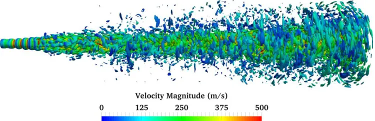
Figure 8: Contour plot of liquid volume fraction represented by an
0.1 isosurface after the jet has penetrated the domain for 15 times. The liquid volume fraction is coloured by velocity magnitude.3.2. Comparison of Coupling simulation
In order to make a consistent comparison in terms of the droplet size distribution
between the RCM and the SCA, the coupling region in the RCM simulation is placed after
z=29.6d which is also the position of the coupling layer in the Grosshans-SCA simulation
[40]. The coupling region extends the length of the computational domain to 41d which is
kept the same as the computational domain used in [40]. Finally, the RCM is employed in the
VOF-LPT coupling region to identify liquid structures suitable for VOF-LPT conversion and
transfer them into the LPT simulation. The simulation is performed for an extended time
equivalent to the jet crossing the entire VOF-LPT domain 10 times. The liquid jet isosurface
together with the converted droplets are displayed in Figure 9. The droplet cloud visualisation
and analysis of the size distribution reveal that most converted droplets have a diameter
between 1 µm and 10 µm, which is consistent with the droplet size distribution obtained by
Grosshans et al. [40] as shown in Figure 10. However, significantly larger quantity of small
droplets (3-8 µm) are identified and extracted by the RCM while SCA produces a droplet size
PDF which shifts more to larger droplet diameters. On the one hand, these differences can be
attributed to the slightly higher breakup intensity predicted by the RCM-VOF method. On the
other hand, indistinguishably converting all liquid structures sampled at the coupling layer
[image:33.595.48.423.101.222.2]ACCEPTED MANUSCRIPT
droplets in the SCA simulation. Since the size of these droplets do not necessarily satisfy the
requirement that a Lagrangian droplet must be smaller than the local grid size, it is more
[image:34.595.48.428.176.299.2]difficult to ensure numerical stability in the SCA than in the RCM.
Figure 9: Atomisation of a simple liquid jet using the RCM method. The 0.1 liquid volume isosurface is coloured in brown while the converted Lagrangian droplets are scaled and coloured according to their diameters.
[image:34.595.47.425.323.608.2]ACCEPTED MANUSCRIPT
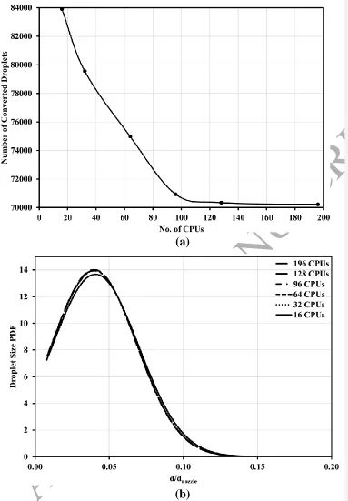
The effects of different decomposition strategies on the identification and extraction
of droplets are demonstrated using 16, 32, 64, 96, 128 and 196 CPU processors. The
simulation time is equivalent to the jet crossing the entire domain 10 times. A scotch method
is employed to ensure that each processor domain is assigned with equal numbers of mesh
elements. The numerical instability in time integration is eliminated by fixing the time step
size at 1.4×10⁻⁹ s for all simulations. As shown in Figure 11(a), decomposing the
computational domain with increasing number of CPUs has a diminishing effect on the
droplet identification and conversion procedures. Moreover, the size distributions of
converted droplets under different decomposing conditions display negligible difference as
depicted in Figure 11(b). These comparisons demonstrates RCM‟s good adaptability to high

![Figure 7ACCEPTED MANUSCRIPT: Plotted average liquid volume fraction along the jet centre line for the RCM-VOF simulation and the Grosshans-VOF simulation [40]](https://thumb-us.123doks.com/thumbv2/123dok_us/8408887.327324/32.595.48.427.274.539/figure-accepted-manuscript-plotted-fraction-simulation-grosshans-simulation.webp)