SUPPLEMENTARY MATERIAL: A RENORMALIZED NEWTON METHOD FOR LIQUID CRYSTAL DIRECTOR MODELING
EUGENE C. GARTLAND, JR∗ AND ALISON RAMAGE†
This note of Supplementary Material extends the modeling, analysis, and numeri-cal experiments of the main paper. The general forms of the macroscopic liquid crystal director models in the presence of electric and/or magnetic fields are discussed; they are carefully compared and contrasted with the Landau-Lifshitz free energy models for ferromagnetic materials; and a typical non-dimensionalization for our prototype problem is presented. In addition, a simple example is given showing that liquid crystal free-energy functionals in general do not possess the kind of “energy decay property” (with respect to rescaling the director field n) that was used in earlier
work to analyze the “Harmonic Mapping Problem.” Finally, we include results from additional numerical experiments, which validate certain properties of the Truncated Newton Method discussed in the main paper.
S1. Liquid crystal director models. Many experiments and devices involving liquid crystal materials can be effectively modeled using a macroscopic continuum framework in which the orientational state of the system is described by a director field(a unit-length vector field representing the average orientation of the molecules in a fluid element at a point), traditionally denoted byn: with respect to an orthonormal
frame,
n=n1e1+n2e2+n3e3, |n|2=n21+n22+n23= 1.
One of the main difficulties in dealing with models such as these numerically is the unit-vector constraint onn, which must be satisfied at each point in the region
oc-cupied by the liquid crystal material. If the director field is simple enough (e.g., a modest tilting or twisting), this can be managed by representing n in terms of
orientation angles (e.g., n= cosθe1+ sinθe2, in a 2-D setting), which recasts the problem as anunconstrained problem for the scalar fields associated with these an-gles. For more complicated director fields, there can be degeneracies associated with the orientation angles, and an angle representation can’t be employed. In such cases, it is common to enforce the constraint |n| = 1 either by Lagrange multipliers or by
penalty methods. Several other liquid crystal models involve unit-length vector fields and constraints—see [8] for more discussion. Standard references on liquid crystals include [2, 3, 9, 10]. Unit-vector constraints arise in other areas as well, including the modeling of ferromagnetic materials—see [4, 6, 7].
S1.1. Coupled electric fields. Most devices and many experiments involve the interaction between a liquid crystal material and an applied electric field (which is used to control the liquid crystal orientational properties). The electric fields are usually created by sandwiching a liquid crystal film between electrodes to which a voltage is applied. This is a coupled interaction, with the electric field influencing the orientations of the liquid crystal molecules and the molecular orientational properties
∗Department of Mathematical Sciences, Kent State University, Kent, Ohio 44242 USA ([email protected]).
in turn influencing the local electric fields through their effect on the dielectric tensor. The free energy (expressed as an integral functional of the field variables) is the thermodynamic potential that determines equilibrium states of systems such as these. For a uniaxial nematic liquid crystal material in equilibrium with a coupled electric field (at constant potential), the free energy has the generic form
F=
Z
Ω
h
W(n,∇n)−1
2D·E
i
, D=ε(n)E, E=−∇U.
Here Ω is the region occupied by the liquid crystal,W is the distortional elastic energy density, Dis the electric displacement (or flux), E is the local electric field,εis the
dielectric tensor, andU is the electrostatic potential.
The form ofW commonly used to model experiments and devices with real (uni-axial nematic) materials is the Oseen-Frank model [9,§2.2], [10,§3.2]:
2W =K1(divn)2+K2(n·curln)2+K3|n×curln|2
+ (K2+K4)
tr(∇n)2−(divn)2
, (S1.1)
where K1, . . . , K4 are material-dependent and temperature-dependent “elastic con-stants.” A simplified form, which embodies the essential features of importance to us here, is the so-called “equal elastic constant” model (K1=K2=K3=K, K4= 0):
W =K 2|∇n|
2
, |∇n|2=
3
X
i,j=1
∂n
i
∂xj 2
, K >0.
The expression for|∇n|2above is for a fixed Cartesian frame. This is the form that
we use in the main paper. We emphasize that this is done for simplicity and does not limit the applicability of the ideas or analysis.
The anisotropy of the medium is reflected in the tensorial nature of the “dielectric constant,” which here corresponds to the real, symmetric, positive-definite tensor field
ε (which is a function of n). At a point in a uniaxial nematic liquid crystal, the ε
tensor is transversely isotropic with respect to the local director n, that is, it has a
distinguished eigenvector parallel tonand a degenerate eigenspace perpendicular to n:
ε(n) =ε0 ε⊥I+εan⊗n
↔ εij =ε0(ε⊥δij+εaninj), εa:=εk−ε⊥. (S1.2a)
In an eigenframe with third eigenvectornat a point, for example, theεtensor would
have Cartesian components
ε=ε0
ε⊥
ε⊥
εk
l,m,n
, l,m,n= orthonormal triple. (S1.2b)
Hereε0is a positive constant, andεkandε⊥are positive, material-dependent, relative
dielectric permittivities (forEoriented “parallel” ton, as opposed to “perpendicular”
to n). For situations involving AC electric fields (with the liquid crystal director
responding to the time-averaged electric field, at sufficiently high frequencies),εkand
ε⊥ would also depend on the frequency of the AC field. The dielectric anisotropyεa
The total free energy of our simplified model then takes the form
F[n, U] = 1
2
Z
Ω
K|∇n|2−ε(n)∇U· ∇U. (S1.3)
This is the simplest prototype model that contains the essential features of importance to us. One can see the intrinsic saddle-point nature of the electric-field coupling: equilibria are minimizing with respect tonbut maximizing with respect to U. In a generic sense, the variational problem has the form
min
|n|=1maxU F[ n, U],
where the extremal elements are sought over sufficiently regular fields that conform to any essential boundary conditions. The strong form of the constrained equilibrium equations for (S1.3) (withεof the form (S1.2)) is
−K∆n=λn+ε0εa ∇U·n∇U, div ε(n)∇U= 0, |n|= 1, (S1.4)
which is to be solved in Ω subject to appropriate boundary conditions on nand U.
The Lagrange multiplier fieldλis associated with the pointwise unit-vector constraint. In terms of Cartesian components (with respect to a fixed frame), the electrostatics equation takes the form
div ε(n)∇U
=X
i,j
∂ ∂xi
εij
∂U ∂xj
= 0.
By virtue of (S1.2), we see that the eigenvalues ofε(n) are independent ofn, are
strictly positive, and are given by
eigenvalues of ε(n) =ε0∗ {εk, εk, ε⊥},
from which follows
ε0min{εk, ε⊥} Z
Ω
|∇U|2≤ Z
Ω
ε(n)∇U· ∇U ≤ε0max{εk, ε⊥} Z
Ω
|∇U|2.
Thus any combination of boundary conditions for U (as well as interface conditions and far-field asymptotic conditions, ifE extends beyond Ω) that yield a well-posed
problem for ∆U = 0 will also give a well-posed problem for div ε(n)∇U= 0.
Assum-ing the auxiliary conditions onU to be such, then, for any given (sufficiently regular) director fieldn, the associated electric potential fieldU is uniquely determined.
In (S1.4) one again sees the coupled nature of the problem, the electric field influencing the director equilibrium solution via the∇Uterms in the first equation and the director field influencing the electric potential throughε(n) in the second equation.
S1.2. Comparison with ferromagnetics. The Landau-Lifshitz free energy provides a phenomenological model for equilibrium states of magnetization in ferro-magnetic materials and bears some similarity to the Oseen-Frank model for liquid crystals [4, 6, 7]. The free-energy density is expressed in terms of a unit-length vec-tor fieldm, which corresponds to a normalized (saturated) magnetization vector M,
analogous to the liquid crystal director nbut differing from it in the sense that m
is aproper vector (m and−marenot equivalent). The density contains terms
pro-portional to|∇m|2, penalizing spatial variations inm(as do the terms inW(n,∇n)
to n). The magnetic stray field is given in terms of a magnetostatic potential via Hs=−∇U (as with the local electric field and electrostatic potential in liquid crys-tals, E =−∇U). The magnetic medium can be regarded as isotropic and
homoge-neous, however, so that the magnetic potential solves ∆U = divM (in the material
domain); whereas the electric potential for liquid crystals satisfies div ε(n)∇U
= 0. This last equation would become div ε(n)∇U= divP in a ferroelectric liquid crystal
with polarizationP.
The contribution of the (spontaneous) stray field to the magnetic free-energy density ispositive (1
2B·Hs, B=µ0(Hs+M)); whereas in a liquid crystal system at constant voltage, the coupling to an applied electric field isnegative (−1
2D·E, D=
ε(n)E). Any externally applied magnetic fieldHe is treated as uniform throughout
the sample and acts as a fixed force (or torque) on the magnetization in much the same way that external magnetic fields influence liquid crystals. Juxtaposing the two free energies (for our model problem with an external magnetic field contribution included), we would have
F[n] = 1
2
Z
Ω
K|∇n|2−ε(n)∇U· ∇U−µ0∆χ(He·n)2
div(ε(n)∇U) = 0 in Ω, plus BCs
versus
F[m] = Z
Ω
h
Cex|∇m|2+µ0
2 |∇U| 2
−µ0He·M + Φ(m)
i
+µ0 2
Z
Rd
\Ω
|∇U|2
∆U =
divM, in Ω
0, in Rd\Ω, plus BCs and interface conditions.
Here µ0 is the vacuum magnetic permeability (the magnetic analogue ofε0), ∆χ is the diamagnetic anisotropy of the liquid crystal material (the magnetic analogue of εa),Cexis the exchange constant, and Φ(m) is the anisotropy energy density of the
ferromagnetic material (a potential favoring certain preferred directions of magneti-zation). See, for example, [9, §2.2 and §2.3] or [10, §3.2 and §4.1] concerning the Oseen-Frank expression, and [4, §1], [6, §1], or [7, Part I, Summary and Results] for the Landau-Lifshitz expression.
Thus, while ferromagnetic systems have to deal with the extended nature of the magnetic stray field and potentialU, they do not have to cope with the indefiniteness (lack of coercivity) that theU variables cause in liquid crystal systems. Furthermore, in the liquid-crystal setting, it is not possible to introduce a Newtonian potential rep-resentation forU, as is done in computational micromagnetics, since the liquid crystal electrostatic problem div(ε(n)∇U) = 0 (or div(ε(n)∇U) = divP) does not reduce
to a Laplace (or Poisson) equation. The combination of inhomogeneity, anisotropy, and negative-definiteness of the coupling between n and U add to the challenge of
S1.3. Non-dimensionalization. It is convenient for analysis and appropriate for numerical explorations in general to express all aspects of the problem (free-energy functional, Euler-Lagrange equations, etc.) in dimensionless form. This renders all variables independent of changes of the system of units employed, reduces the total number of parameters, and identifies the combinations of parameters upon which the equilibrium solutions actually depend. If the problem were to be left in fully dimensional form, then the vectors of unknowns in the discretized model in the paper would contain mixtures of quantities of different physical dimensions, and the norms of those vectors that are employed in our analysis would need to contain additional weight factors to balance these physical dimensions appropriately.
As an example of a reasonable non-dimensionalization, consider the model free-energy functional F in (S1.3) in d space dimensions (Ω ⊂ Rd). The director n is
dimensionless by definition, as are εk and ε⊥, their difference εa, and the relative
dielectric tensor
εr:= 1
ε0ε=ε⊥I+εan⊗n.
One can scale lengths by the diameter of Ω and scale the electrostatic potential by the applied voltage V,
xi :=
xi
L, L:= diam(Ω), U := U V,
to obtain the following dimensionless form:
F[n, U] = 1
2
Z
Ω
|∇n|2−α2εr(n)∇U· ∇U
, F := F
KLd−2, α 2
:= ε0V 2
K .
Here Ω is the domain Ω in the rescaled coordinate system, and∇is the spatial gradient operator with respect to the rescaled coordinates (∇ =L−1∇). The functional has the same form as before in (S1.3) but now withK= 1 andε0=α2(and all quantities dimensionless). The Euler-Lagrange equations (S1.4) would transform in a similar way. In the paper, we assume that the problem has been non-dimensionalized in a reasonable way such as this, but we drop the overbars for convenience of notation.
S2. Lack of an energy decay property in general. Those familiar with the analysis of the “harmonic mapping case” in [1] will wonder if any of those results are relevant to the analysis in the main paper here. We address this now. The “Harmonic Mapping Problem” is a special case of the types of models we consider here. It consists of a normalized equal-elastic-constant model with no magnetic or electric fields (the “Dirichlet Energy”):
F[n] =1
2
Z
Ω
|∇n|2, minF[n], subject to|n|= 1 in Ω, n=n0on∂Ω.
In [1], a convergence analysis was presented for an iterative scheme that involved a renormalization step (n←n/|n|) similar to that employed in Algorithm 4.1 in the
main paper. The analysis relied upon the fact that renormalizing a director field that is greater than unit length necessarily reduces the Dirichlet energy:
Unfortunately, this decay property seems to be tied to the simple form of the Dirichlet energy and does not hold for liquid crystal free-energy functionals in general. To see this, consider, for example, an equal-elastic-constant model with an external magnetic field:
F[n] =1
2
Z
Ω
K|∇n|2−µ0∆χ(H·n)2
, H= const, K, µ0,∆χ >0. (S2.1)
If n is un-normalized with |n| ≥ 1 on Ω, then rescaling n ← n/|n| will lower the
contribution of the distortional elasticity (|∇n|2 term) but will increase (make less negative) the contribution of the magnetic energy density ((H·n)2term). Thus one may have in principle either F[n/|n|] ≤ F[n] or F[n/|n|] > F[n]. For the special
case of rescalingnin (S2.1) by aconstant multiplicative factor, we would have
F[cn] =c2F[n], c= const,
for which
|c|<1 andF[n]<0 ⇒ F[cn]>F[n].
It is common to have negative free energies for stable liquid crystal equilibrium director fields with external magnetic fields or coupled electric fields, and this is the case, for example, with all Fr´eedericksz-transition problems (classical magnetic-field or electric-field induced distortions) beyond the “switching threshold”—see for example [9,§3.4 and§3.5] or [10,§4.2].
We do not know under what circumstances one can have an energy decay property for the general Oseen-Frank distortional elastic energy density (S1.1) (with unequal elastic constants), even in the absence of magnetic or electric fields. The problems mainly of interest to us (with coupled electric fields) are not even free-energy min-imization problems. They are minimax problems, and our analysis in §4.1 of the main paper applies to any regular saddle-point equilibrium solution of such problems (locally stable or unstable).
S3. Numerical experiments on the Truncated Newton Method. Numer-ical experiments were conducted to explore some aspects of the Truncated Newton Method (as discussed in §4.3 and §4.4): spectral properties of the projected Hessian H(n) of (4.18) and solutions of the Truncated Newton step H(n)p =−G(n). For this we used the same model problem (5.1), discretized as in (5.3). WithN = (n−1)2 total free nodes, the projected HessianH(n) is 3N×3N, and the projected gradient G(n) is a 3N-vector. Proposition 4.6 of§4.4 indicates that for a regular constrained discrete equilibrium solution n∗ of this model problem, the nullity of H(n∗) should be equal toN. This was borne out for small-scale examples for which the full set of eigenvalues ofH(n∗) could be computed using Matlab’s eigensolver for full (dense) ar-rays, utilizing solution vectorsn∗that were computed to machine attainable accuracy by the Renormalized Newton Method solver. Results are reported in Table S3.1 for n= 4 using a fully converged upward “escape” solution forn∗. In this case,N = 9, H(n∗) is 27×27, and the first nine eigenvalues are of the order of the machine epsilon, while the last 18 eigenvalues are order one.
Table S3.1
Eigenvalues of the projected HessianH(n∗)(4.18) of the Truncated Newton step (4.19) evalu-ated at a fully converged “escape” solutionn∗(see§5.1 and Fig. 5.1 right) forn= 4andN = 9. H(n∗)is27×27, and the eigenvalues are scaled and given in increasing sequence, left to right, top to bottom. The eigenvalues were calculated using Matlab’seig()function.
scale scaled eigenvalues ofH(n∗) 10−15
−1.06 −0.88 −0.57 −0.49 −0.43 −0.16 0.34 0.87 1.20
1 0.55 0.59 0.98 1.59 1.97 2.27 2.52 2.53 2.92
1 3.18 3.52 3.54 4.00 4.06 4.66 4.71 5.56 5.69
Table S3.2
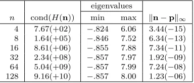
Numerical aspects of the Truncated Newton stepH(n)p=−G(n) (4.19) for the model Har-monic Mapping Problem (5.1), discretized as in (5.3). Heren is the crude initial guess for the upward “escape” solution (5.6) with α = 0.6, and H(n) is the projected Hessian of the Trun-cated Newton Method (4.18). 1-norm condition numbers were estimated using Matlab’scondest() function, and minimum and maximum eigenvalues ofH(n)were computed using Matlab’seigs() function. pis the solution of H(n)p=−G(n)computed using Matlab’s backslash operator (with H(n)stored as a symmetric sparse Matlab array).
eigenvalues
n cond(H(n)) min max kn−pk∞
4 7.67(+02) −.824 6.06 3.44(−15)
8 1.64(+05) −.846 7.52 6.34(−13)
16 8.61(+06) −.855 7.88 7.34(−11)
32 2.34(+08) −.857 7.97 1.92(−09)
64 5.04(+09) −.857 7.99 7.24(−08)
128 9.16(+10) −.857 8.00 1.23(−06)
forn= 4,8, . . . ,128. Also computed were the 1-norm condition number ofH(n) (es-timated by Matlab’s condest()function), the minimum and maximum eigenvalues of H(n) (computed by Matlab’s eigs() function), and the max norm of the dif-ference between the computed solution vector p and the true solution n (for H(n) nonsingular). The results are reported in Table S3.2. The projected Hessian H(n) was found to be indefinite but nonsingular, although ill-conditioned with condition numbers much larger than those of M and ZTAZ in Table 5.5. The condition
num-bers grow with nbut don’t appear to follow a regular scaling law. The relationship between cond(H(n)) andkn−pk∞for the different values ofnis as one would expect (in double precision).
REFERENCES
[1] F. Alouges,A new algorithm for computing liquid crystal stable configurations: the harmonic mapping case, SIAM J. Numer. Anal., 34 (1997), pp. 1708–1726.
[2] S. Chandrasekhar,Liquid Crystals, Cambridge University Press, Cambridge, 2nd ed., 1992. [3] P. G. de Gennes and J. Prost,The Physics of Liquid Crystals, Clarendon Press, Oxford,
2nd ed., 1993.
[4] C. J. Garc´ıa-Cervera,Numerical micromagnetics: A review, Bol. Soc. Esp. Mat. Apl., 39 (2007), pp. 103–135.
[5] E. C. Gartland, Jr., H. Huang, O. D. Lavrentovich, P. Palffy-Muhoray, I. I. Smalyukh, T. Kosa, and B. Taheri,Electric-field induced transitions in a cholesteric liquid-crystal film with negative dielectric anisotropy, J. Comput. Theor. Nanosci., 7 (2010), pp. 709–725. [6] M. Kruˇz´ık and A. Prohl,Recent developments in the modeling, analysis, and numerics of
ferromagnetism, SIAM Review, 48 (2006), pp. 439–483.
[7] A. Prohl,Computational Micromagnetism, Teubner, Stuttgart, 2001.
director modeling, SIAM J. Sci. Comput., 35 (2013), pp. B226–B247.
[9] I. W. Stewart,The Static and Dynamic Continuum Theory of Liquid Crystals: A Mathe-matical Introduction, Taylor and Francis, London, 2004.