ESSAYS ON EMPIRICAL ASSET PRICING USING BAYESIAN METHODS

City, University of London Institutional Repository

Citation

: Rubesam, A. (2009). ESSAYS ON EMPIRICAL ASSET PRICING USING

BAYESIAN METHODS. (Unpublished Doctoral thesis, City University London)

This is the accepted version of the paper.

This version of the publication may differ from the final published

version.

Permanent repository link:

Link to published version

:

Copyright and reuse:

City Research Online aims to make research

outputs of City, University of London available to a wider audience.

Copyright and Moral Rights remain with the author(s) and/or copyright

holders. URLs from City Research Online may be freely distributed and

linked to.

1

ESSAYS ON EMPIRICAL ASSET PRICING

USING BAYESIAN METHODS

by

Alexandre Rubesam

A Thesis Submitted in Partial Fulfilment of the Requirements for

the Degree of

Doctor of Philosophy

CITY UNIVERSITY

Faculty of Finance, Cass Business School

January/2009

Supervisor: Dr. Soosung Hwang

2

List of Tables ... 4

List of Illustrations ... 6

Acknowledgements ... 7

Copyright waiver... 8

Abstract ... 9

Chapter 1 - Introduction... 10

Chapter 2 – Is Value Really Riskier Than Growth? ... 19

2.1. Introduction... 19

2.2. Regime-Switching Model ... 25

2.2.1. Lower Partial Moment CAPM... 25

2.2.2. Higher Moment CAPM... 27

2.2.3. Regime-Switching Model with Alternative Risk Measures ... 28

2.2.4. Estimation Method... 31

2.3. Empirical Results ... 32

2.3.1. Data ... 33

2.3.2. Preliminary Results with Unconditional Models... 35

2.3.3. Is Value Riskier than Growth? Reinvestigation with Market Regimes ... 37

2.3.4. Regime-Switching Risk Measures... 44

2.3.5. Robustness Checks... 50

2.4. Conclusion ... 53

References... 70

Chapter 3 – The Disappearance of Momentum ... 74

3.1. Introduction... 74

3.2. Modelling Structural Changes in Premia ... 78

3.2.1. Multiple Change-Point Model ... 78

3.2.2. Estimation ... 81

3.2.3. Bayes Factors ... 84

3.3. Empirical Results ... 85

3.3.1. Momentum Returns ... 85

3.3.2. A Preliminary Analysis: Momentum in Five-Year Subsamples... 88

3.3.3. Momentum Premium and Structural Breaks... 89

3.3.4. Is the Recent Period Unusual? ... 94

3.3.5. Discussion: Delays in the Disappearance of Momentum ... 96

3.4. Momentum Premium During Boom and Bust ... 98

3

3.6. Appendix... 105

3.6.1. Gibbs Sampling Scheme ... 105

3.6.2. Calculating the Marginal Likelihood ... 109

References... 132

Chapter 4 – Fishing with a Licence: an Empirical Search for Asset Pricing Factors ... 135

4.1. Introduction... 135

4.2. Methodology ... 141

4.2.1. Stochastic Search Variable Selection... 141

4.2.2. Interpreting the Posterior Results... 145

4.2.3. Research Design... 146

4.3. Empirical Results ... 151

4.3.1. Data ... 151

4.3.2. Exploratory Analysis of the Factors ... 154

4.3.3. Selection of Asset Pricing Factors ... 155

4.3.4. Robustness ... 160

4.3.5. Summary and Comparison with Previous Studies... 161

4.4. Conclusion ... 162

4.5. Appendix: Detailed Explanation of Prior and Posterior Distributions... 164

4.5.1. Prior Distributions... 165

4.5.2. Gibbs Sampling Scheme ... 166

4

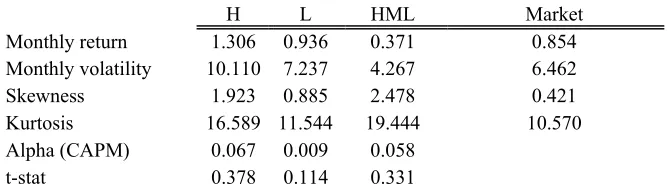
Table 2-1 Descriptive statistics of value, growth and value-minus-growth portfolios

... 55

Table 2-2 OLS regressions of CAPM, LCAPM (Lower Partial Moment CAPM) and

HCAPM (Higher-moment CAPM) ... 56

Table 2-3 Descriptive statistics of value, growth and value-minus-growth portfolios

in different market regimes ... 58

Table 2-4 OLS regressions of CAPM value, growth and value-minus-growth

portfolios in different market regimes... 59

Table 2-5 Estimation results for the regime-switching model with alternative risk

measures... 60

Table 2-6 Average value-minus-growth return and market return per regime ... 61

Table 2-7 Descriptive statistics of additional value, growth and value-minus-growth

portfolios ... 62

Table 2-8 OLS regressions of CAPM, LCAPM (Lower Partial Moment CAPM) and

HCAPM (Higher-moment CAPM) for additional portfolios in different market regimes ... 63

Table 2-9 Estimation results for the regime-switching model with alternative risk

measures for additional portfolios... 64

Table 2-10 Average value-minus-growth return and market return per regime for

additional portfolios ... 65

Table 3-1 Summary statistics of portfolios sorted on past returns ... 114

Table 3-2 Momentum returns in 5-year non-overlapping subsamples... 116

Table 3-3 Log-marginal likelihoods and differences in log-marginal likelihoods of

models with different numbers of change-points... 117

Table 3-4 Parameter estimates - WMLCRSP 6x6 portfolio ... 118

Table 3-5 Log-marginal likelihoods of multiple change-point models for several

momentum portfolios... 119

Table 3-6 Estimation of the multiple change-point model for various momentum

portfolios ... 120

Table 3-7 Bootstrap estimation of the probability of observing the momentum

premium over the period from January 2001 to December 2006 ... 123

Table 3-8 Contribution of different sectors of the economy to momentum returns 124

Table 3-9 The Effect of the Hi-Tech Bubble on the profitability of momentum.... 125

Table 4-1 Summary statistics of candidate factors... 170

Table 4-2 Exploratory Analysis of the Factors Using OLS ... 171

Table 4-3 Marginal posterior probabilities of factors and model posterior probability

5

Table 4-4 Marginal posterior probabilities of candidate factors and model posterior

probabilities for 55 portfolios ... 174

Table 4-5 Marginal posterior probabilities of candidate factors and model posterior

probabilities for 30 industry portfolios ... 176

Table 4-6 Marginal posterior probabilities of factors and model posterior probability

for individual stocks (c = 10) ... 178

Table 4-7 Marginal posterior probabilities of factors and model posterior probability

6

Figure 2-1 Smoothed probabilities of market regimes - Full Sample (July 1926 to

December 2006)... 66

Figure 2-2 Smoothed probabilities of market regimes - Post-Depression Sample

(July 1935 to December 2006)... 66

Figure 2-3 Smoothed probabilities of market regimes - Post-1963 Sample (July 1963

to December 2006)... 67

Figure 2-4 Smoothed probabilities of market regimes - Pre-1963 Sample (July 1926

to June 1963)... 67

Figure 2-5 Smoothed probabilities for the regime-switching model with alternative

risk measures... 68

Figure 3-1 Posterior probabilities of regimes for the WMLCRSP,6x6 strategy... 126

Figure 3-2 Contribution of different sectors of the economy to momentum returns

... 127

Figure 3-3 Contribution of hi-tech, telecom and all other stocks to momentum

returns... 128

Figure 3-4 Average momentum returns excluding the contribution of hi-tech, and

telecom stocks ... 129

Figure 3-5 Average returns of a momentum strategy that does not allow hi-tech and

telecom stocks ... 130

Figure 3-6 Cumulative profits of several momentum strategies through December

7

Acknowledgements

I am very grateful to Dr. Soosung Hwang for his invaluable guidance and support. I would also like to thank the academic and general staff at Sir John Cass Business School.

This research could not have been done without the financial support from the Coordenação de Aperfeiçoamento de Pessoal de Nível Superior (CAPES), a Brazilian governmental agency which sponsored this project. I am thankful to them and to the Brazilian taxpayers, who are ultimately responsible for that support.

I would like to thank my direct and extended family and specially my parents, who have supported my decision to pursue a PhD degree in many ways.

I would like to thank my friend Dr. Helder Parra Palaro, with whom I have shared the experience of higher education over the last 10 years.

8

Copyright waiver

9

Abstract

This thesis is composed of three essays related to empirical asset pricing. In the first essay of the thesis, we investigate recent rational explanations of the value premium using a regime-switching approach. Using data from the US stock market, we investigate the risk of value and growth in different market states and using alternative risk measures such as downside beta and higher moments. Our results provide little or no evidence that value is riskier than growth, and that evidence is specific to pre-1963 period (including the Great Depression). Within the post-1963 sample, there are periods when the value premium can be explained by the CAPM, whilst during other periods the premium is explained by the fact that the returns on value firms increase more than the returns on growth stocks in periods of strong market performance, whilst in downturns growth stocks suffer more than value, and these features are captured by different upside/downside betas or higher moments. These results are not consistent with a risk-based explanation of the value premium.

The second essay of the thesis contributes to the debate about the momentum premium. We investigate the robustness of the momentum premium in the US over the period from 1927 to 2006 using a model that allows multiple structural breaks. We find that the risk-adjusted momentum premium is significantly positive only during certain periods, notably from the 1940s to the 1960s and from the mid-1970s to the late 1990s, and we find evidence that momentum has disappeared since the late 1990s. Our results suggest that the momentum premium has been slowly eroded away since the early 1990s, in a process which was delayed by the occurrence of the high-technology stock bubble of the 1990s. In particular, we estimate that the bubble accounts for at least 60% of momentum profits during the period from 1995 to 1999.

10

C

C

h

h

a

a

p

p

t

t

e

e

r

r

1

1

I

I

n

n

t

t

r

r

o

o

d

d

u

u

c

c

t

t

i

i

o

o

n

n

The ultimate task of asset pricing, as Cochrane (2001) puts it, is “to understand and measure the sources of aggregate or macroeconomic risk that drive asset prices”. Advances in theory over the last 50 years - as well as the ever-increasing availability of large amounts of data and cheap computational power - have expanded our understanding of how asset prices behave enormously. However, one could argue that this task remains unfinished.

11

portfolio (i.e. the CAPM alpha) is significantly positive, the researcher concludes that this is evidence against the CAPM. Three cases in particular have received a vast amount of attention from academic works, namely the so-called size, value and momentum effects, which refer to the inability of the CAPM to price portfolios formed on market capitalisation, the ratio of book to market equity and past returns, respectively.

The presence of these empirical irregularities is interpreted in a variety of ways. Whilst some researchers believe that they indicate the presence of market inefficiencies or biased investor behaviour and perception, others believe that they represent additional sources of risk which are not captured by the CAPM beta. Another possibility is that they are the result of data-snooping, i.e. by looking at thousands of possible firm characteristics, researchers have found some which are related to average returns by sheer chance. The debate about the value premium is illustrative of these different views. Fama and French (1993, 1996), for instance, argue very strongly that the value effect is related to a financial distress risk factor, but other studies (e.g. Lakonishok, Shleifer and Vishny (1994)) argue in favour of the behavioural story. Fama and French further propose a three-factor model including the market return and two additional factors related to the size and value effects. The idea that multiple risk factors are important to determine asset prices is incorporated in the theories of the Intertemporal CAPM of Merton (1973) and the Arbitrage Pricing Theory of Ross (1976). These theories, however, are silent as to which and how many these factors might be, and this is left as a largely empirical issue.

12

whether they are related to non-diversifiable risk. The second is to identify, amongstst many empirical possibilities, which should be used as risk factors in asset pricing models. The first two essays in this thesis are related to the first issue, specifically to the value and momentum anomalies. The third essay is related to the second issue; in particular, which factors should be included in a linear factor model to prices stock returns.

The first essay in this thesis, entitled Is Value Really Riskier Than Growth?,

contributes to the debate surrounding the value premium. It is a commonly-held belief that growth options are riskier than assets in place, because growth options depend more on future and uncertain economic conditions. However, value firms (whose values come mostly from existing assets) earn higher average returns than growth firms (whose values comes mostly from growth options) but have lower betas in the post-1963 period. The value premium has drawn considerable attention from both academics and practitioners alike. Academics would like to definitively explain the source of the premium. If the value premium is, as Fama and French (1993) advocate, related to a real, aggregate, non-diversifiable source of risk, academics would like to understand exactly what this risk is. Practitioners, on the other hand, are concerned with whether, if genuine, this anomaly is going to persist in the future.

13

a role for time-varying risk in explaining the premium, the empirical evidence in that respect is mixed.

14

We investigate a number of value, growth and value-minus-growth portfolios from the US stock market. Our results do not support the risk-based explanation of the value premium. When we identify the market state through regimes extracted from the market return, there is little or no difference in the risk of value-minus-growth portfolios across market states, and this difference does not explain the value premium. The analysis with different risk measures suggests that, in the post-1963 period, there are periods when the value premium can be explained by the CAPM, and other periods when the returns on value stocks increase much more than those on growth stocks, which is captured by different upside/downside betas or higher moments. Our results also suggest that the value premium is likely to be high during periods of bad market performance because of the negative returns of the growth portfolio.

In the second essay of this thesis, entitled Disappearance of Momentum, we

investigate whether momentum strategies have been consistently profitable over time. The momentum anomaly has been a major focus of research since the publication of an influential paper by Jegadeesh and Titman (1993), who documented that simple strategies that buy stocks that had high returns in the previous 3 to 12 months and short stocks that had low returns in the same period earn an abnormal return of approximately 1% per month over a holding period of up to 12 months. How and why such a profitable opportunity appeared to persist for such a long period of time is a perplexing question; in an efficient market, arbitrageurs are expected to quickly drive away these profits.

15

momentum premium is significantly positive only during certain periods of time. Particularly, the last structural break we find occurred around the year 2000, and since then the momentum premium becomes insignificant. Also, although there have been periods of insignificant momentum premium in the past, we find that the momentum premium in this recent period is not probable considering the past distribution of momentum premia, which indicates that the anomaly might have been eroded away.

16

500 to more than 9000, and the assets under management by these funds has risen from 50 billion to over 1.5 trillion US dollars1.

Finally, in the last essay in this thesis, Fishing with a Licence: an Empirical

Search for Asset Pricing Factors, we investigate which factors should be included in

a linear factor model to explain stock returns. We use a Bayesian approach to calculate posterior probabilities of possible factors. Our methodology is based on a Bayesian variable selection procedure from the statistics literature called Stochastic Search Variable Selection (SSSV), introduced by George and McCulloch (1993). We extend their approach to a simple multivariate case with N assets, i.e. we are

interested in calculating the posterior probabilities of factors to explain many assets simultaneously. Our approach has several advantages. First, our method focuses on obtaining the posterior probabilities of the more promising models directly, without the need to estimate the posterior probabilities of all possible models, which can be quite an overwhelming task considering the growing number of possible factors. Second, it allows us to use data on thousands of individual stocks, which is important considering the data-snooping biases inherent when factors created by sorting on variables are tested on portfolios related to these variables (Lo and MacKinlay (1990), Ferson, Sarkissian and Simin (1999) and Berk (2000)).

We test 12 factors that have been reported in the literature. These are: the excess market return, size, value, momentum, asset growth, idiosyncratic volatility, trading volume, long-term reversal, liquidity, coskewness, cokurtosis and downside risk. We apply our methodology to a large number of individual stocks as well as portfolios of stocks from the US market. Our results suggest that a linear factor model for stock returns should contain the excess market return, the size factor and

17

the liquidity factor. We find only weak evidence that the idiosyncratic volatility, the value/growth and the downside risk factors should be included. Also, our results with individual stocks and portfolios of stocks differ dramatically. The posterior probability of the Fama and French (1993) value/growth factor (HML) is high only when it is estimated with portfolios formed using the book-to-market ratio, but the size factors (SMB) has high posterior probability regardless of the assets used.

References

Bawa, Vijay S., and Eric B. Lindenberg, 1977, Capital market equilibrium in a mean-lower partial moment framework, Journal of Financial Economics 5,

189-200.

Berk, Jonathan B., 2000, Sorting out sorts, The Journal of Finance 55, 407-427.

Black, Fischer, 1972, Capital market equilibrium with restricted borrowing, The

Journal of Business 45, 444-455.

Cochrane, John, 2001, Asset pricing (Princeton University Press, Princeton and

Oxford).

Fama, Eugene F., and Kenneth R. French, 1993, Common risk factors in the returns of stocks and bonds, The Journal of Financial Economics 33, 357-384.

Fama, Eugene F., and Kenneth R. French, 1996, Multifactor explanations of asset pricing anomalies, The Journal of Finance 51, 55-84.

Ferson, Wayne E., Sergei Sarkissian, and Timothy T. Simin, 1999, The alpha factor asset pricing model: A parable, Journal of Financial Markets 2, 49-68.

George, Edward I., and Robert E. McCulloch, 1993, Variable selection via gibbs sampling, Journal of the American Statistical Association 88, 881-889.

Harlow, W. V., and K. S., Rao, 1989, Asset pricing in a generalized mean-lower partial moment framework: Theory and evidence, The Journal of Financial

and Quantitative Analysis 24, 285-311.

18

Jegadeesh, N., and Sheridan Titman, 1993, Returns to buying winners and selling loosers: Implications for stock market efficiency, The Journal of Finance 48,

65-91.

Kraus, A., and R. H. Litzenberger, 1976, Skewness preference and the valuation of risky assets, The Journal of Finance 31, 1085-1100.

Lakonishok, Josef, Andrei Shleifer, and Robert W. Vishny, 1994, Contrarian investment, extrapolation, and risk, The Journal of Finance 49, 1541-1578.

Lintner, J., 1965, The valuation of risk assets and the selection of risky investments in stock portfolios and capital budgets, The Review of Economic and

Statistics 47, 13-37.

Lo, A. W., and A. C. MacKinlay, 1990, Data-snooping biases in tests of financial asset pricing models, Review of Financial Studies 3, 431-468.

Markowitz, H., 1952, Portfolio selection, The Journal of Finance 7, 77-91.

Merton, R. C., 1973, An intertemporal asset pricing model, Econometrica 41,

867-887.

Ross, S. A., 1976, An arbitrage theory of capital asset pricing, Journal of Economic

Theory 13, 341-360.

Sharpe, W. S., 1964, Capital asset prices: A theory of market equilibrium under conditions of risk, The Journal of Finance 19, 425-442.

19

C

C

h

h

a

a

p

p

t

t

e

e

r

r

2

2

I

I

s

s

V

V

a

a

l

l

u

u

e

e

R

R

e

e

a

a

l

l

l

l

y

y

R

R

i

i

s

s

k

k

i

i

e

e

r

r

t

t

h

h

a

a

n

n

G

G

r

r

o

o

w

w

t

t

h

h

?

?

2.1.

Introduction

20

Fama and French (1993, 1995) argue that HML is a risk factor which represents financial distress of weak firms with low earnings, which tend to have high book-to-market ratios. On the other hand, Lakonishok, Shleifer and Vishny (1994) suggest investors’ incorrect extrapolation of the past earnings growth of firms as the source of the value premium. Others try to explain the premium in the framework of the CAPM, with mixed results. For example, Jagannathan and Wang (1996) and Ang and Chen (2007) propose conditional CAPM models. Lewellen and Nagel (2006) and Petkova and Zhang (2005) also use conditional CAPM models to investigate the value premium, but their results are not as strong as those of Ang and Chen (2007). Campbell and Vuolteenaho (2004), on the other hand, decompose the beta of a stock into the ‘good’ beta that comes from news about the discount rate and the ‘bad’ beta from news about the future cash flows, and show that value stocks have higher proportion of ‘bad’ betas. Some of these studies, however, have been criticised by Daniel and Titman (2005), who show that their favourable results could be due to the low power of the tests used.

21

provided in the firm or industry level using firm characteristics. Xing and Zhang (2005) show that value firms in the manufacturing sector perform worse than growth firms in the negative business cycle and vice versa, using variables such as earnings growth, sales growth, investment growth, and investment rate, whilst Cooper, Gerard and Wu (2005) investigate the link between the rate of capacity and the degree of investment irreversibility and the book-to-market ratio.

One caveat with the empirical studies above is that they use subsets of stocks, whilst the value premium is calculated using a much larger number of stocks from the whole market. For example, the number of manufacturing firms Xing and Zhang (2005) use in their study is only 21% (37% in market capitalisation) of the firms publicly traded in the market. In addition, the firm characteristics used by these studies may reflect business cycles, but are not necessarily concurrent with the movements in financial markets because the lead and lag relationship between the firm characteristics and the dynamics in the stock market is not likely to be constant.

Some of the studies mentioned above attempt to model time-varying risk and the expected market risk premium directly. We do not follow this path for two reasons. First, as mentioned before, studies based on this approach fail to show conclusive evidence that time-varying risk explains the value premium. Second, the choice to use a conditional model and to estimate the expected market risk premium involves either a subjective decision about which conditioning variables to use, or a high degree of model parameterisation (as in Ang and Chen (2007)).

22

different mean market returns and volatilities. This approach allows us to study the risk of the value-minus-growth strategy in different market conditions, whilst avoiding a high degree of parameterisation and subjective choices of conditioning variables. Specifically, we investigate the risk of value and growth by estimating the CAPM conditioned on the state of the market as inferred from the regime-switching model of the market return. If value is riskier than growth during bad states when the market is doing poorly, there should be an increase in the beta of HML in the corresponding market regime2.

The approach above, however, may be criticised in two points. First, this analysis assumes that the risk of HML is related to the state of the economy as measured by the market regimes. Even if the risk of HML is not related to the different market regimes, there could still be increases (decreases) in this risk over different periods. Second, using beta as the measure of risk might not be adequate, since investors are not likely to have quadratic utility and asset returns do not follow the normal distribution. If the investors’ utility function is better specified by power utility and higher moments such as skewness and kurtosis matter in asset return distribution, asymmetry or fat tails should be priced. These asymmetric risk measures might be particularly relevant, considering that value and growth are expected to react differently to periods of good and bad economic conditions. Therefore we consider the possibility that different risk measures other than the CAPM beta, such as the downside beta and higher moments, matter to explain portfolios’ returns over time, without the explicit assumption that they must be related to the state of the market or economy.

23

Several asset pricing models have been proposed to explain asymmetry and fat tails. Amongst these, we choose two widely known equilibrium asset pricing models in addition to the CAPM: the lower partial moment CAPM (henceforth LCAPM) and the higher moment CAPM (henceforth HCAPM). The LCAPM, which was developed by Bawa and Lindenberg (1977) and Harlow and Rao (1989), includes asymmetric reactions to downside and upside markets separately. Chan (1988), De Bondt and Thaler (1987), and Petkova and Zhang (2005) use it to investigate the value premium but give us mixed results. The HCAPM introduced by Kraus and Litzenberger (1976) prices higher moments. A closely related study is Harvey and Siddique (2000) who model conditional skewness. Higher moments explain asset returns with asymmetry or fat tails, but are not necessarily the same as the upside and downside betas.

One major difference of the approach above from those of previous studies is that any of the three models − CAPM, LCAPM, and HCAPM − can explain asset returns in the regime switching framework we employ. Since these are based on equilibrium models, our approach is still within the rationality framework. Thus we seek explanations on the value premium in the conventional risk-return framework by concentrating on the empirical possibility of changing risk measures and its impact on asset pricing. When there are no differences in upside and downside betas or when higher moments are not priced, the model is equivalent to the conventional CAPM. Therefore the LCAPM or HCAPM are selected only when asymmetries or fat tails matter in asset pricing.

24

asymmetric models should show that the downside beta is higher than upside beta for value-minus-growth portfolios during bear markets or that the coefficients on higher moments should be significant during bear markets such that value firms become riskier.

Our results show that, when we identify the market state through a regime-switching model for the market return, there is little or no difference in the risk of value-minus-growth portfolios across market regimes, and this difference does not explain the value premium, except when the pre-1963 sample (including the Great Depression) is used. Moreover, when we investigate the value premium using different risk measures, we find that there are periods of time when the premium can be explained by the CAPM, whilst during other periods the premium is explained by the fact that the returns of value firms increase more than the returns on growth stocks in periods of strong market performance, whilst in downturns growth stocks suffer more than value stocks. These features are captured by the upside/downside betas in the LCAPM or by the coefficient on the square and cube of the market return in the HCAPM. Overall, our results are not consistent with a risk-based explanation of the value premium.

25

2.2.

Regime-Switching Model

In this section we first explain different risk measures and why they could be used to model the value premium. We then introduce a regime switching model that allows these risk measures to be used over time, and the method used to estimate it.

2.2.1.

Lower Partial Moment CAPM

Previous studies test either betas, consumption betas or conditional betas of value-minus-growth portfolios as the relevant measure of risk. However, the asymmetric reactions of value and growth firms to market conditions, proposed by Zhang (2005), might not be well explained by symmetric models such as the CAPM. An alternative model to test this theory would be the downside/upside CAPM, which allows different response to positive and negative market movements.

This upside/downside CAPM model (the Lower Partial Moment CAPM, LCAPM) initially developed by Bawa and Lindenberg (1977) and Harlow and Rao (1989), has been a popular method to investigate asymmetric reactions to market movements or if downside beta is priced.3 This model suggests that investors react differently to the returns above or below a specified target return:

pt LCAPM mt mt t

r =α +β− −r +β+ +r +ε , (2.1)

26

where r_pt is the excess return on portfolio p, r_mt =R_mt −r_f is the excess market

return, rmt r I rmt

(

)

+ _{= > and}

(

)

target mt mt mt

r− =r I r <r are the positive and negative

components of the excess market return relative to the target return r_target, I(.) is the

indicator variable, and ε_t is an error term with mean zero and standard deviation σ_p. Although the LCAPM has an appealing property for the explanation of asymmetry in asset returns, there are a few issues which remain unclear. First, this model cannot be directly estimated through OLS using equation (2.1), due to the issue discussed in Post and Van Vliett (2005): if the constant is included, the downside and upside betas calculated by OLS are not consistent with what the

LCAPM suggests4.Consequently, throughout this study, we first estimate β− and β+ _{by running a regression without the constant to obtain the estimates that are}

consistent with the LCAPM theory, and then calculate ˆα_LCAPM using these estimates

as the mean and standard error of the residuals αˆ_LCPAM =r_pt −βˆ+ +r_mt −βˆ− −r_mt. Second,

there is no agreement about how we should define the upside and downside markets that are inherently unobservable. Popular methods are setting the target return to zero or to the average market return. Petkova and Zhang (2005) obtain four market states (peak, expansion, recession, and trough) depending on the expected market risk premium calculated with four macroeconomic variables. Although this method is consistent with theory and thus appealing, the estimated market premium could be noisy, and the breakpoints between peak and expansion and between recession and

27

trough, i.e. 10% and -10%, are arbitrary. We will come back to this issue later in Section 2.3.3.

2.2.2.

Higher Moment CAPM

Alternative risk measures could be obtained by generalising the assumption of the CAPM, i.e. the unrealistic mean-variance assumption based on normality or quadratic utility function. Assume that asset returns are non-normal and investors’

utility function is not quadratic, which we believe is more realistic than normality or a quadratic utility function. The utility function can be linearised using the Taylor series expansion assuming compact returns (see Ingersoll (1987)). In equilibrium the expanded utility function is equivalent to the CAPM only when moments higher than the second moment are trivial. In general, for investors whose utility function is linear risk tolerant, asset prices need to be modelled by the CAPM with additional higher moment terms. The requirement of the additional terms depends on the probability density function of asset returns, which changes over time. Although both the HCAPM and LCAPM can model asymmetry in asset returns5, the HCAPM models returns as a non-linear function of the market return, whilst in the LCAPM asset returns are priced linearly with market returns conditioning on up- and down-markets. Therefore the two models are not necessarily the same and in particular, the HCAPM can be used to price kurtosis in addition to skewness in asset returns.

28

There are several different approaches to include higher moments (see for example Kraus and Litzenberger (1976), Friend and Westerfield (1980), Sears and Wei (1985), Barone-Adesi (1985), Harvey and Siddique (2000)). As explained in Kraus and Litzenberger (1976) and Hwang and Satchell (1999), we use the following cubic market model which is consistent with the four moment (coskewness and cokurtosis) CAPM. The specification is:

( )

(

)

(

( )

)

1 2 3

pt HCAPM mt mt mt mt mt t

r =α +βr +β R −E R +β R −E R +ε . (2.2)

2.2.3.

Regime-Switching Model with Alternative Risk Measures

We consider three equilibrium based models, i.e. the traditional CAPM, the LCAPM that allows different responses to up- and down-market states and the HCAPM that models skewness and fat tails in addition to the traditional beta. Empirically, most of the previous studies test one of these models against the other models for certain sample periods and then conclude which one explains assets’ returns better than the others. For example, beta appears to be priced before 1968 (Fama and MacBeth (1973)), but not from 1963 to 1990 (Fama and French (1992)). Lim (1989) reports that skewness is priced in some sub-periods. These empirical results indicate that asset returns are priced with different risk measures for different time periods.

29

decreasing absolute risk aversion as in Arrow (1971). Moreover assume that both the probability density function of asset returns and the investors’ degree of risk aversion change over time (Campbell and Cochrane (1999)). Then, in this generalised framework the choice of risk measures does not lie in selecting one that dominates the others for the entire sample period, but in finding out which one is selected over time. When asset returns are normally distributed for a specific period of time, for example, the CAPM explains asset returns. However, when asset returns become non-normal, i.e. skewed or fat-tailed, and investors become far more risk averse, assets are priced not only by mean and variance but also by higher moments or downside risk. Therefore, different risk measures may be required for different periods of time to explain asset returns.

In order to model asset returns with different risk measures over different periods of time, we assume that there are N regimes defined by S_t, a random

Markov regime variablethat for each time t assigns a value in

{

}

dummy variable S_jt, j=1, 2, …, N, is defined for each regime, that is, S_jt =1when

t

S = jand Sjt =0 otherwise, our model is given by

1 N

pt p jt jt pt

j

r α S m ε

=

= +

∑

where m_jt is a fully-specified relationship between the portfolio return r_pt, and the

set of factors in regime j, and ε_pt ~ 0,

(

)

1 N

pt p j jt j

S

σ σ

=

=

∑

For m_jt the following three models are used. First, for the CAPM we have

1t mt

30

Following the discussion in subsections 2.2.1 and 2.2.2, we allow the LCAPM and the HCAPM to be selected by defining

2t mt mt

m =β− −r +β+ +r (2.5)

and

( )

(

)

(

( )

)

3t 1mt 2 mt mt 3 mt mt

m =βr +β R −E R +β R −E R . (2.6)

When the data generating processes follow equations (2.4), (2.5) and (2.6), they are

equivalent to the CAPM, LCAPM, and HCAPM, respectively. Therefore, our regime

switching model can be presented as:

[

]

( )

(

)

(

( )

)

1 2

2 3

3 1 2 3

pt p t mt t mt mt

t mt mt mt mt mt pt

r S r S r r

S r R E R R E R

α β β β

β β β ε

− − + +

⎡ ⎤

= + + _⎣ + _⎦

⎡ ⎤

+ _⎣ + − + − _⎦+ (2.7)

Note that the transition probability matrix will describe how likely it is to migrate from one regime, say the CAPM, to another, say, the HCAPM. Since we specify a first-order Markov chain, the only information that matters to predict the regime at time t+1 is the regime at time t.

This regime-dependent risk measure model is quite flexible since asset returns can be modelled with time variation in both asset returns’ distribution and investors’ risk aversion. Over different periods of time, any one of the models can dominate the other two, or there may be no dominant model. The estimates of the parameters and probabilities of regimes could provide answers to the questions of whether and when value firms are riskier than growth firms; e.g. by comparing β,

β−_{, and β}+_{of value and growth portfolios. If β}− _>β+ _{in the LCAPM during bear}

31 2 0

β < (β₂ >0) in the HCAPM, the portfolio is expected to show lower returns

(higher returns) and be riskier (less risky) than other portfolios that just follow the CAPM. If β₃>0 (β₃ <0) and market returns are positively skewed, the portfolio is

expected to show higher (lower) returns than the symmetric CAPM and the portfolio is less risky (riskier).

2.2.4.

Estimation Method

We estimate the regime-switching model (2.7) via a Bayesian Markov Chain Monte Carlo (MCMC) Gibbs-sampling approach. As Kim and Nelson (1999) point out, using the Gibbs sampler to estimate unobserved variables as well as parameters allows us to draw from the relevant distributions simultaneously. Moreover, the model has conditioning features that make it simple to implement the Gibbs sampler. Another reason to use an MCMC method is that it provides posterior distributions from which we draw the parameter estimates and conduct significance tests directly. Finally, by averaging the generated values of the regime dummy variables we obtain estimates of the smoothed probabilities of regime selection over time, which are useful to study the implications of our model.

The Gibbs sampling estimation of model (2.7) consists of two steps. Let

(

)

− +

=

θ denote the vector of parameters in the

model. In the first step, conditional on θ, we sample from the distribution of

(

)

T = S ST

S% _K using the multi-move algorithm of Carter and Kohn (1994).

32

breaks, so in the second step each parameter in θ is sampled in turn, conditioned on these structural breaks. We use standard conjugate Gaussian distributions for the regression coefficients and the inverted gamma distribution for the variance, as in Zellner (1971). Given the issue discussed in Section 2.2.1, we take special care to draw β− and β+from the correct distributions (i.e. these parameters are drawn from

the distribution which disregards the constant term, so that correct downside and upside betas are estimated). The transition probabilities are estimated using conjugate beta priors. We allow for a large number of burn-in iterations to guarantee convergence. All results are obtained with 10,000 iterations after 30,000 burn-in iterations.

2.3.

Empirical Results

33

2.3.1.

Data

There are many different ways of constructing value/growth portfolios. Book-to-market, earnings and other firm characteristics have been used with different breakpoints in the literature. We focus on several widely used value, growth and value-minus-growth portfolios.

The main results in this paper are reported for two sets of portfolios. The first set of portfolios are Fama and French’s (1993) H (high book-to-market or value portfolio), L (low book-to-market or growth portfolio), and HML (value-minus- growth) portfolios, which are constructed using a two-by-three sort on size and book-to-market. HML has been used as a standard measure of the value premium since Fama and French (1993), and has been used in many studies, including Petkova and Zhang (2005) and Fama and French (2006a). The second set of portfolios considers size, since the value premium is supposedly stronger amongst smaller firms (Loughran (1997) and Fama and French (2006a)). From a five-by-five sort on size and book-to-market the small-value (Hs) and small-growth (Ls) portfolios can be calculated, and the small value premium HMLs is the small-value portfolio (Hs) minus the small-growth portfolio (Ls). To check the robustness of our results, we also use portfolios based on a decile sort on earnings-to-price ratio6. The excess market return is the CRSP value-weighted portfolio return minus the one-month Treasury bill rate. All the data are obtained from Kenneth French’s data library.7

6 _{Fama and French (2006a) show that the value premium becomes less dependent on size if earnings-to-price ratio is used} instead of book-to-market ratio

34

We consider different subsamples within the period from July 1926 to December 2006: the full sample (1926-2006), the post-depression sample (1935-2006), and the post-1963 sample (1963-2006). We focus more on the post-1963 sample because the value premium is more difficult to explain during this period. The value premium in the period from 1926 to 1963 can be explained using the simple CAPM or the conditional CAPM; see Ang and Chen (2007) and Fama and French (2006a). We consider the post-depression sample because the Great Depression was a remarkably unique event which could alter the results significantly. In our robustness checks we also consider the pre-1963 sample.

The value premium can be measured by average returns or unconditional alphas of value-minus-growth portfolios. Table 2-1 reports several descriptive statistics for our portfolios. Consistent with previous studies, i.e. Fama and French (1992, 1993, 2006) and Davis, Fama and French (2000), the value premium exists and is stronger for small stocks. The value premia from HML and HMLs in the full sample (Panel A) are, in terms of average returns (CAPM alphas), 0.42% and 0.51% (0.32% and 0.48%), respectively. When we exclude the Great Depression (Panel B), the value premia from the HML and HMLs portfolios increase to 0.48% and 0.56% (0.51% and 0.66%) in terms of average returns (unconditional alphas). Finally, in the more recent period from 1963 to 2006 (Panel C), the average returns (unconditional alphas) of the HML and HMLs portfolios still remain high, at 0.45% and 0.62% (0.58% and 0.80%), respectively.

35

value portfolios have larger skewness than the growth portfolios and thus the value-minus-growth portfolios have positive skewness.

2.3.2.

Preliminary Results with Unconditional Models

In this subsection we investigate the value premium with OLS estimation of the CAPM, LCAPM and HCAPM. Panels A, B and C of Table 2-2 report the results using the full, post-depression and post-1963 periods, respectively. From the estimates of the CAPM, there is very little evidence that value is riskier than growth; indeed, the betas of HML and HMLs are positive only when the sample includes the Great Depression (see Panel A), whilst in the post depression and post-1963 samples betas are negative and mostly significant (Panels B and C).

Accounting for different responses to up- and down-markets reduces alpha significantly. The LCAPM alphas are much smaller than the CAPM alphas in all three samples. For instance, in the full sample the LCAPM explains the value

premium ( ˆα_LCAPM = −0.15%, t-stat = -1.39), whilst the CAPM does not

( ˆα_CAPM =0.32%, t-stat = 2.69). This results has been obtained by Chan (1988), De

Bondt and Thaler (1987) and was replicated in Petkova and Zhang (2005). Value stocks seem to benefit from a larger increase in returns in up-markets and a smaller

decrease in returns in down-markets (i.e. β+ >β−), whilst growth stocks behave in

the opposite way (β− >β+). However, value is not riskier than growth in any of the

36

the downside betas are negative and statistically significant. Specifically, in the post-1963 sample, the downside betas of HML and HMLs (-0.36 and -0.50) are roughly double the upside betas (-0.17 and -0.22), so during this period we expect the value-minus-growth strategies to have high and positive returns when the market return is negative, but negative returns when the market return is positive.

Higher moments seem to be significant mostly when the sample includes the Great Depression. In the full sample, the coefficients of HML on the square and cube of the market return are positive and significant. However, they do not represent risk; the positive coefficient on the square market return (b₂) suggests that the return on

HML increases further when the market return is positive, but decreases less when market returns are negative. Also, since the market has positive skewness in the full sample (Panel A, Table 2-1), HML increases even further with the positive b₃. The

HCAPM seems to reduce the size and significance of the premium; for instance over the full sample, the CAPM alpha is 0.32% (t-stat = 2.69) but the HCAPM alpha is lower at 0.25% and borderline significant (t-stat = 2.00). The higher moments are not significant in the post-depression samples, but are significant for the growth portfolios in the post-1963 sample, increasing their risk relative to the CAPM.

37

2.3.3.

Is Value Riskier than Growth? Reinvestigation with Market

Regimes

In this subsection we reinvestigate if value is riskier than growth in different market states. As pointed out earlier, we first show that market states derived from the estimated expected market risk premium may be too noisy. For example, Petkova and Zhang (2005) obtain market states from estimates of the expected market risk premium obtained with macroeconomic variables. Although they argue this is a better measure of the market return than ex-post returns, it is not clear whether the lagged four macroeconomic variables could provide unbiased and noise-free estimates of the expected market risk premium.

To investigate this, as in Petkova and Zhang (2005), we run Center for Research in Security Prices (CRSP) value-weighted market returns in excess of one month Treasury Bill rate (rmt) on the following four lagged macroeconomic

variables: the one month Treasury Bill (TBill), credit spread (CS) (the difference between Moody's AAA and BAA rated corporate bonds), term spread (TS) (the difference between the US 10 year and the 1 year treasury bond rates), and dividend yield (DY) (the CRSP value-weighted dividend yields).8 _{For the period between} January 1963 and December 2004 (504 monthly observations) we have

, 1 0.0004 2.211_{(0.060) (1.432)} 1.461_(2.053) 0.042_(0.178) 0.084_(0.072) ˆ , 1

m t t t t t m t

r ₊ = − TBill + CS + TS − DY +ε ₊ (2.8)

38

where the numbers in brackets are the Newey-West heteroskedasticity consistent t

statistics.9 None of the lagged macroeconomic variables are significant at the 1% level, and only one lagged variable, CS, is significant at 5% level.10 Moreover, the value of R-square is only 1.85%. In other words, less than 2% of ex post market

returns reflects ex ante market returns if the regression is a proper way to estimate

the expected market returns. These results suggest that even though we admit that individual beliefs are not homogeneous (Ross (1978)), the difference between ex post

and ex ante returns appears to be too large to justify using the simple regression to

approximate the expected market returns. In addition, by including variables (such as DY, TS, and TBill) that do not appear to explain next month excess market returns, the estimated market risk premium is likely to have large measurement errors. Although the four macroeconomic variables are economically motivated and thus are widely used in the literature (see e.g. the discussion in Ferson, Sarkissian and Simin (2003)) , we could not conclude that the estimated expected market return from the regression is a good proxy for the expected market risk premium. This is supported by Cooper and Gubellini (2008), who show that the results from conditional models (including the one used by Petkova and Zhang (2005)) are extremely sensitive to the conditioning variables used.

9 _{Further studies on the properties of these four macroeconomic variables suggest that the augmented Dick-Fuller test fails to} reject that TBill and DY have unit root. Thus as shown by Ferson, Sarkissian and Simin (2003), the regression results may be further undermined by the high level of autocorrelation in these independent variables.

39

2.3.3.1.Regime Switching Models for the Market Return

We consider a different approach to identify the market states, which is motivated by the regime-switching literature and the modelling of business cycles. Following Hamilton (1989) and Schwert (1989), Turner, Startz and Nelson (1989) and Hamilton and Susmel (1994) show that there are distinct regimes in the S&P 500 index in terms of mean and volatility. Moreover, Hamilton and Lin (1996) investigate the relationship between stock returns and real output growth in industrial production, and conclude that economic recessions are the primary drivers of fluctuations in market volatility. More recently, Perez-Quiros and Timmermann (2000) use regime-switching models to study the risk of firms with different sizes in expansions and recessions. These studies suggest that regime switching models are an effective tool to identify regimes which are linked to economic conditions.

We model the data-generating process of the market return as a three-state first-order Markov process with switching mean and variance11. Our model for the market return can be described in the following way. Let St be a regime variable

assuming the values of 1, 2 or 3 according to the appropriate regime, and

(

)

jt t

S =I S = j be dummy variables which assume the value of 1 when the market is

in regime ,j j=1, 2,3, where I(.)is the indicator variable. The model is then given by

1 1 2 2 3 3 ,

2 2 2 2

, ,1 1 ,2 2 ,3 3

,

mt t t t m t t

m t m t m t m t

r S S S

S S S

µ µ µ σ ε

σ σ σ σ

= + + +

= + = (2.9)

40

where µ_j and σ_{m j,} are the expected excess market return and volatility, respectively,

in regime j. Following Hamilton (1989), we allow the regime variable S_{t to be}

governed by a first-order Markov chain with a transition probability matrix

{ }

P= p where p_ij =P S

(

)

followed by regime j at time t. We interpret each regime according to estimates of

the mean and volatility of the market.

2.3.3.2.Description of Market Regimes

We estimate the regime-switching model for the three sample periods using the Bayesian MCMC Gibbs-sampling estimation, which is standard from the regime-switching literature (see Kim and Nelson (1999) for example). From the MCMC estimates of the dummy variable S_t, we estimate the smoothed probabilities of the

41

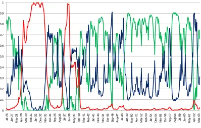
For example, for the full sample, the average monthly market return in the bull and bear markets are 1.26% and -059%, respectively, whilst the volatilities are 2.95% and 11.19% (see the column labelled “Market” in Table 2-3). Figure 2-1 shows that the bear market regime is selected mostly during the Great Depression and during the period from the middle of 1937 through the middle of 1940, which includes the first two years of the Second World War, and then during short periods such as the 1973 oil crisis and the Black Monday month of October 1987. When we exclude the Great Depression period (Figure 2-2), we find that the bear market regime now includes many other periods.

In the post-1963 sample (Figure 2-3), the bear market regime captures periods such as the two oil crises, the Mexican moratorium of 1982, the Black Monday of 1987, the Russian crisis of 1998, the burst of the internet bubble and the period following the terrorist attacks of 2001. The bull regime includes most of the economic expansion of the US economy in the early 1960s, and also most of the early 1990s. The overall picture we obtain with these results is that the return on the aggregate stock market can be modelled as a mixture of longer expansion or bull market periods with high returns and low volatility (the mean market return and volatility in the bull regime are 1.57% and 3.53%), and infrequent and shorter periods of contraction during which the stock market does very poorly and has high volatility (the mean market return and volatility in the bear regime are -1.54% and 6.34%), which agrees with the modelling of regimes and the business cycle using macroeconomic data as in Hamilton (1989).

42

(0.53% in terms of average return) when the market is in the bull market regime and lowest (0.19%) when the market is in the bear regime (the difference in the median HML across regimes is statistically significant at 1%). However, in the more recent post-1963 period, we find that, as expected from the estimates of the LCAPM for this period (Panel C, Table 2-2), the average HML return is higher in the bear market regime, at 1.21% a month) and actually negative in the bull market regime (these differences are also statistically significant). Therefore, over the last 40 years, growth stocks do marginally better than value stocks during bull markets, but do much worse than value stock in the bear market regime. This is contrary to what one expects from the theory of Zhang (2005)12_.

2.3.3.3.The Value Premium in Different Market Regimes

We now proceed to investigate the risk of the value, growth and value-minus-growth portfolios in different market states. We estimate the CAPM conditioned on the state of the market (transition, bull or bear). The purpose of this subsection is to investigate the asymmetric reactions of value and growth firms to market conditions suggested by Zhang (2005).

Panels A, B and C of Table 2-4 report the estimation results for the H, L and HML portfolios using the full, post-depression and post-1963 periods, respectively13_. The risk of the value portfolio increases during bear market only if the sample includes the period of the Great Depression. When we exclude the Great Depression

43

(Panel B), value is not riskier than growth in any of the regimes, whilst alpha is positive and statistically significant in the bull and transition regimes. In the post-1963 sample (Panel C), value is significantly less risky than growth in the bull and bear regimes, whilst in the transition regime beta is not statistically different from zero. Also, as expected, the value premium is very strong in the bear market regime (the bear-market alpha is 0.82%, t-statistic 2.56), but not very strong in the bull regime (the bull-market alpha is only 0.31% and not statistically significant).

44

2.3.4.

Regime-Switching Risk Measures

The results so far have revealed no conclusive empirical evidence supporting Zhang’s (2005) theory or Petkova and Zhang’s (2006) result that value is riskier than growth in bad times. In this subsection we investigate whether or not our regime switching model with different risk measures can capture the asymmetric risk pattern of HML over time. We combine the three models (CAPM, LCAPM and HCAPM) in the regime-switching model in Equation (2.7), so each model has the possibility of being selected in each month. If there are periods when the relationship between the portfolios and the market is symmetric, then the CAPM should be selected. Asymmetries can be modelled by two alternative models: either in dichotomous up and down markets (LCAPM) or in a continuous framework (HCAPM).

We estimate the regime-switching model (2.7) for the H, L, HML, Hs, Ls and HMLs portfolios for the post-1963 sample. We focus on this sample for a few reasons. First, as stated before, the value premium is more difficult to explain during this period. Second, there is a structural break in the early 1960s (see for instance Section 3.1 of Petkova andZhang (2005), and Figure 1 of Fama French (2006)), and thus using a long time series without considering the breaks could be misleading. Our earlier results also confirm that including the Great Depression period could give us wrong inferences about the value premium for the last 40 years. Finally, our regime switching model allows different classes of risks, but not time-varying risks within a regime.

45

probabilities in Figure 2-5 can be interpreted as the probability that, at each month, the CAPM, LCAPM and HCAPM are selected.

It is important to note that the regime switching risk measures explain the value premium in terms of alpha. The posterior distributions of the alphas of HML and HMLs suggest that HML and HMLs can be explained by the model at the 1% significance level. In the next subsection, we show that the value premium is explained by the higher upside betas of the value-minus-growth portfolios, relative to their downside betas, and the positive coefficient on the squared and cubed market returns. This result suggests that it is not increased downside risk during bearish markets which drives the value premium. In the following subsections, we examine the risk of the value portfolio and the value premium in more detail.

2.3.4.1.Is Value Riskier than Growth?

From the estimates in Table 2-5, there is no evidence that value is riskier than growth in any of the regimes. First, the CAPM beta is negative (and significant) for both portfolios: for HML (HMLs) the average posterior beta is -0.16 (-0.28), with a standard deviation of 0.07 (0.05). Second, in the LCAPM regime, the downside betas of both portfolios are also negative and significant. The downside beta of HML (HMLs) is -0.69 (-0.87), with a standard deviation of 0.16 (0.14). Finally, in the HCAPM regime, beta is not significantly different from zero for either of the value-minus-growth portfolios, but the coefficients on the square and cube of the market return are positive and statistically significant14_{. A positive coefficient on the second}

46

moment of excess market return makes HML concave to market movements, increasing returns whilst decreasing risk.

These estimates also suggest that the average HML (HMLs) return might be higher in the LCAPM and HCAPM regimes. In the LCAPM regime, this is expected because even though both the downside and the upside betas are negative, the downside beta is larger than the upside beta, so the return on HML will increase more when the market return is negative than it will decrease when the market return is positive15. In the HCAPM regime, in addition to the increase due to the positive coefficient on the squared market return, the positive coefficient on the third moment of excess market returns increases the returns of HML even further because the market has positive skewness in this regime (not reported).

Table 2-6 displays the average HML and HMLs returns in each of the three regimes. The t-statistics show whether the average return within a regime is significantly different from that of the whole sample. The average value-minus-growth returns in the CAPM regime are significantly lower than those of the whole period: they are only 0.01% and -0.10% for HML and HMLs respectively. As expected, in the LCAPM and HCAPM regimes the average returns are much higher and in some cases significant. We examine whether these differences are significant with a non-parametric median test for robustness, since we do not know the distribution of market returns within a regime. The hypothesis that the median return is the same across regimes is rejected at the 1% significance level for both HML and HMLs. On the other hand, the difference in market returns across regimes is not significant.

47

48

2.3.4.2.Selection of Regimes

In this subsection we study the selection of each regime through time. The transition probabilities tell us how likely it is to remain in each model (i.e. the CAPM, LCAPM or HCAPM) or to move to another one. Also, we analyse the smoothed probabilities that each regime has been selected at each month.

The regimes are persistent for all portfolios except the L portfolio. Figure 2-5 shows that for the L portfolio, the only persistent regime is the LCAPM regime. Since the higher moment coefficients are not significant, and the betas in the CAPM and HCAPM regimes are very close, the L portfolio could be well described by a model with two regimes (CAPM and LCAPM). So there are periods when growth stocks behave similarly in up and down markets, and other periods when downside risk is increased. For the H portfolio, all regimes are persistent, as indicated by the transition probabilities.

The HML and HMLs portfolios tend to exhibit similar (but weaker) patterns to the H and Hs portfolios, respectively (see Figure 2-5). It should be noticed that, in the case of portfolio Hs, the HCAPM regime is quite persistent, even though the higher moments are not significant. The estimate of beta in this regime, though, is much smaller than in the CAPM regime, so we can attribute the persistence to the difference in beta.

49

close to zero (for HML) or negative (for HMLs) when the CAPM regime is selected, that is, when the relationship between the return on the value-minus-growth strategies and the return on the market is symmetrical. This regime is selected over short one or two-year long periods, with the exception of two longer periods, one in the late 1970s and another from 1985 to 1992. Overall, this is the most prevalent regime: it is selected in 241 (249) months when the model is estimated with the HML (HMLs) portfolio, which corresponds to almost half of the whole sample. Therefore, the value premium is close to zero during half of the post-1963 sample.

The LCAPM regime is selected during some turbulent periods, such as the oil crisis of 1973 and a four-year period following the burst of the internet bubble in 2000. The average excess return on the H and L portfolios during this regime are 0.66% and -0.45%, respectively, and thus much of the HML return during this period comes from the negative returns of growth firms.

The HCAPM is the least persistent regime for both HML and HMLs; the probability of remaining in this regime (p₃₃) is 0.84 and 0.82 for the HML and

HMLs portfolios respectively. This regime is selected in 131 (120) months for the HML (HMLs) portfolio, which corresponds to around 25% (22%) of the whole sample. It is selected over short periods, usually less than a year, except for the period from the middle of 2003 until early 2005.

50

2.3.5.

Robustness Checks

So far we have reported results obtained using two sets of portfolios, both of which are based on sorting procedures using market equity and the book-to-market ratio. We have also focused more on the more recent sample period from 1963 onwards. We address the first issue by replicating our results using value, growth and value-minus-growth portfolios based on a decile sort on Earnings/Price ratio. We define the highest decile to be the value portfolio (H_EP) and the lowest decile to be the growth portfolio (L_EP), and the value-minus-growth portfolio (HML_EP) is the H_EP portfolio minus the L_EP portfolio. To address the second issue, we replicate our results for the pre-1963 sample period, using the H, L and HML portfolios.

2.3.5.1.Portfolios Formed on Earning/Price Ratio

51

reported on Table 2-8. Similarly to our previous results in Table 2-4, value (H_EP) is not riskier than growth (L_EP) in any of the market regimes, and alpha is large in the bear and transition regimes (although it is not statistically significant in the bear regime).

Finally, we estimate the regime-switching model with different risk measures for the H_EP, L_EP and HML_EP portfolios. The results are reported in Panel A of Table 2-9 and are quite similar to those obtained before. In Panel A of Table 2-10, we repeat our analysis of the average value premium and market return in each regime, and the results are also similar to those obtained with the HML portfolio: the value premium is highest in the LCAPM regime, at 1.29%, and nearly zero in the CAPM regime at 0.08%. It is also very high in the HCAPM regime, at 0.93%. As with the results for the HML portfolio, the difference in the median HML_EP return across regimes is statistically significant.

2.3.5.2.The Pre-1963 Period