City, University of London Institutional Repository
Citation:
Andrienko, G., Andrienko, N., Bremm, S., Schreck, T., Von Landesberger, T.,
Bak, P. and Keim, D. (2010). Space-in-time and time-in-space self-organizing maps for
exploring spatiotemporal patterns. Computer Graphics Forum, 29(3), pp. 913-922. doi:
10.1111/j.1467-8659.2009.01664.x
This is the unspecified version of the paper.
This version of the publication may differ from the final published
version.
Permanent repository link:
http://openaccess.city.ac.uk/2847/
Link to published version:
http://dx.doi.org/10.1111/j.1467-8659.2009.01664.x
Copyright and reuse: City Research Online aims to make research
outputs of City, University of London available to a wider audience.
Copyright and Moral Rights remain with the author(s) and/or copyright
holders. URLs from City Research Online may be freely distributed and
linked to.
City Research Online:
http://openaccess.city.ac.uk/
[email protected]
Eurographics/ IEEE-VGTC Symposium on Visualization 2010 G. Melançon, T. Munzner, and D. Weiskopf
(Guest Editors)
Volume 29(2010),Number 3
Space-in-Time and Time-in-Space Self-Organizing Maps for
Exploring Spatiotemporal Patterns
G. Andrienko1, N. Andrienko1, S. Bremm2, T. Schreck2, T. von Landesberger2,3, P. Bak4, D.Keim4
1University of Bonn & Fraunhofer IAIS, Germany 2Technische Universität Darmstadt, Germany
3Fraunhofer IGD, Germany 4University of Konstanz, Germany
Abstract
Spatiotemporal data pose serious challenges to analysts in geographic and other domains. Owing to the complex-ity of the geospatial and temporal components, this kind of data cannot be analyzed by fully automatic methods but require the involvement of the human analyst’s expertise. For a comprehensive analysis, the data need to be considered from two complementary perspectives: (1) as spatial distributions (situations) changing over time and (2) as profiles of local temporal variation distributed over space. In order to support the visual analysis of spa-tiotemporal data, we suggest a framework based on the "Self-Organizing Map" (SOM) method combined with a set of interactive visual tools supporting both analytic perspectives. SOM can be considered as a combination of clustering and dimensionality reduction. In the first perspective, SOM is applied to the spatial situations at differ-ent time momdiffer-ents or intervals. In the other perspective, SOM is applied to the local temporal evolution profiles. The integrated visual analytics environment includes interactive coordinated displays enabling various transfor-mations of spatiotemporal data and post-processing of SOM results. The SOM matrix display offers an overview of the groupings of data objects and their two-dimensional arrangement by similarity. This view is linked to a cartographic map display, a time series graph, and a periodic pattern view. The linkage of these views supports the analysis of SOM results in both the spatial and temporal contexts. The variable SOM grid coloring serves as an instrument for linking the SOM with the corresponding items in the other displays. The framework has been validated on a large dataset with real city traffic data, where expected spatiotemporal patterns have been suc-cessfully uncovered. We also describe the use of the framework for discovery of previously unknown patterns in 41-years time series of 7 crime rate attributes in the states of the USA.
Categories and Subject Descriptors(according to ACM CCS): H.1.2 [User/Machine Systems]: Human information processing—Visual Analytics; I.6.9 [Visualization]: Information Visualization—
1. Introduction
Spatiotemporal data pose serious challenges to analysts. Firstly, owing to the complexity of the geographical space, data having a geospatial component cannot be adequately analyzed by fully automatic methods, but require the in-volvement of the human analyst’s sense of the space and place, tacit knowledge of their inherent properties and rela-tionships, and space / place -related experiences [AAD∗08]. These are incorporated into the analysis through the use of an appropriate representation of the space such as a carto-graphic map, which serves as a model of the reality through
The analysis of spatiotemporal data may be, however, too complex for humans: the number of distinct places can be too large, the time period under analysis too long, and/or the attributes depending on space and time too numerous. There-fore, human analysts require a proper support from compu-tational methods capable to deal with large and multidimen-sional data.
Comprehensive analysis of spatiotemporal data requires consideration of the data in a dual way [AA05b]:
• As a temporally ordered sequence of spatial situations. A
spatial situationis a particular spatial distribution of ob-jects and/or values of attributes in some time unit (i.e. mo-ment or interval);
• As a set of spatially arranged places where each place
is characterized by its particular temporal variation of at-tribute values and/or presence of objects. We shall call it
local temporal variation.
Accordingly, there are two high-level (synoptic) subtasks in analysis of spatiotemporal data:
• Analyze the change of the spatial situation over time, i.e. temporal evolution of the situation.
• Analyze the distribution of the local temporal variations over space.
In order to support both tasks, we suggest a framework for analyzing spatiotemporal data with the use of the computa-tional method called Self-Organizing Map (SOM) [Koh01]. SOM combines clustering with dimensionality reduction: objects are not only grouped but also arranged in one- or two-dimensional space according to their similarity in terms of multidimensional attributes. We have built a visual an-alytics environment in which it is possible to apply SOM to spatial situations and temporal variations and explore the results obtained by means of various visual and interactive techniques.
An overview of related research concerning the use of SOM for visual data exploration is given in Section2. Sec-tion3describes our tools for spatiotemporal analysis with the use of SOM. In Section4, we describe an application of the tools to real data about city traffic in Milan with pre-viously expected spatiotemporal patterns. We demonstrate that the tools allowed us to detect these patterns. In Sec-tion5, we show how these tools allow uncovering previously unknown spatiotemporal patterns in another real dataset de-scribing crimes in the USA. This is followed by a discussion of our contribution in comparison to the state of the art and conclusion in Section6.
2. Related work
The SOM methodology is discussed in depth in Kohonen’s
monograph [Koh01]. The Self-Organizing Map is a neural
network type vector projection and quantization algorithm.
By means of a competitive, iterative training process, a net-work of prototype vectors (or neurons, or cells) is trained (adjusted) to the input vector data. The output of the algo-rithm is a network of vectors that is approximately topology preserving w.r.t. the input data. The network can be inter-preted as a set of clusters and simultaneously as a map to lay out the input data elements (e.g., in the nearest neigh-bor sense w.r.t. the prototypes). Typically, two-dimensional rectangular or hexagonal prototype vector networks are as-sumed. The SOM algorithm is usually outperformed in terms of vector quantization capability by algorithms not requiring the network constraint. On the other hand, the capability of SOM to arrange input data in a regular network structure provides good opportunities for visualization. This makes the method very convenient for integration in an environ-ment for interactive visual exploration of multidimensional data. To date, SOM has been successfully used for a number of visual analysis applications.
The SOM method is applicable to any data type that can be represented by vectors. Specifically, complex and multimedia data can be addressed by SOM if represented by appropriate feature vector data. A few example applica-tions to name in this respect include financial data [DK98], text [ND06], images [Bar08], or time-dependent scatter data [SBvLK09]. Vesanto [Ves99] describes the basic analytic tasks that can be addressed with SOM and options for SOM visualization supporting these tasks. The tasks include anal-yses of cluster structure, of prototype vectors, and of overall data distribution.
The SOM method has been successfully applied in the geospatial data analysis domain, where its data aggregation and sorting properties are leveraged. A wealth of applica-tions are described in a recent book on the topic [AS08]. As the SOM network itself represents an abstract map for data, color-coding can be used to link the location of data elements in SOM space with their respective geospatial
co-ordinates [KK08,ST08]. VISSTAMP is a system linking
views based on geospatial maps, SOM maps, parallel coor-dinate and table plots [GCML06]. Besides using simple lin-early scaled two-dimensional color maps, approaches exist for advanced mappings adjusting for non-uniform
distribu-tions of SOM distances [KVK00] and considering
percep-tual issues [GGM∗05]. Variants of the SOM algorithm exist that include also geospatial coordinates in the SOM train-ing process, allowtrain-ing a tradeoff of multivariate and geospa-tial data properties in the obtained SOM [BLP05]. An inter-esting way of linking SOM to geographical space and time is described in [Sku08]. A trajectory made by a person in the geographical space is projected onto the space of SOM where geographical places are arranged according to their similarity in terms of multiple attributes.
G. Andrienko et al. / Space-in-time and time-in-space SOMs 3
values in order to find the archetypal distributions for a re-gion and then looks for certain temporal patterns such as fre-quencies of the archetypes in dry and wet years. Hewitson does not consider the complementary analytic task, analysis of the spatial distribution of the local temporal variations.
In [GCML06], SOM is applied to combinations of val-ues of multiple attributes characterizing pairs <place + time unit>. Assessing similarities and differences among spatial situations is done by visual inspection of multiple maps (one map per time unit) where each place has the color of the SOM cell containing the particular combination of this place and the time unit. Assessing similarities and differ-ences among local temporal variations is done using a re-orderable matrix where the rows correspond to the places, columns to the time units, and cells have the colors of the SOM nodes. Hierarchical clustering groups the rows by sim-ilarity; however, the spatial context is missing. We apply SOM to spatial situations and temporal variations; hence, the results directly match the analytic tasks.
3. Description of the tools
We have integrated the SOMPAK SOM engine [KHKL96]
in a visual analytics environment for spatiotemporal analy-sis. The environment supports transformations of spatiotem-poral data, controlling the work of the SOM algorithm, post-processing of the SOM results, and putting the results in the spatial and temporal contexts for human interpretation.
The Self-Organizing Map method is used for grouping and arranging spatial distributions and temporal variation profiles according to their similarity. The results are pre-sented in the SOM matrix display. Two-dimensional color mapping links the SOM matrix with additional data views for supporting multi-perspective data analysis. Thus, the car-tographic map display represents SOM results in the geo-graphical context. For this purpose, places in the map are colored according to the positions of the respective profiles of local temporal variation in the SOM matrix. Two types of temporal displays, time graph and time arranger, repre-sent SOM results in the temporal context. For this purpose, segments of these displays are colored according to the posi-tions of the respective spatial situaposi-tions in the SOM matrix. The time arranger supports detection of periodic temporal patterns in the occurrence of similar spatial situations.
The system also includes interactive tools for spatiotem-poral aggregation and other data transformations, which may be needed for preparing data to the application of the SOM method and for interpreting the results obtained. Examples of the use of these tools are given in Sections4and5.
3.1. Parameterization of SOM Algorithm
The SOM algorithm requires a number of parameters to be set. We distinguish between the network size (number of
prototype vectors) and training parameters (including learn-ing rate and neighborhood kernel function). Suitable train-ing parameters can be set accordtrain-ing to the empirical rule-of-thumb recommendations [KHKL96]. An alternative is to automatically evaluate a series of different parameterizations and take the best result as judged by an objective SOM qual-ity measure such as quantization or topology error. We re-gard the network size as a user-chosen parameter. Typically, it will depend on the user task and data size. If the data set is large and data reduction is desired, the number of proto-types is set much smaller than the number of data items, thus providing data aggregation. If the data set is rather small, the network size may be set about equal to the number of data items. In this case, the SOM algorithm mainly acts as a similarity-preserving layout method.
In principle, different parameterizations may give differ-ent results in terms of prototype vectors and their layout in the network. However, we practically observe that the results are rather stable even over larger parameter varia-tions. If desired, stability can further be enhanced by data-dependent and supervised training initialization methods (see [Koh01,KHKL96]).
In our system, we apply the rule-of-thumb parameteriza-tions suggested in [KHKL96] for training and let the user select the network size interactively. For simplicity of the implementation, we stick to a rectangular SOM network. While SOMPAK is an efficient implementation, depending on the data size and training parameterization, SOM calcula-tion runtime may not be interactive. While for our data sets, runtimes were quite fast, we note that interactive SOM cal-culation is not a necessity in our application.
3.2. SOM matrix display
We apply the SOM method to two types of complex ob-jects: (1) spatial situations that occurred in different time units, and (2) local temporal variations that occurred in dif-ferent places. Accordingly, there are two variants of SOM
outcomes called ’space-in-time SOM’ and ’time-in-space
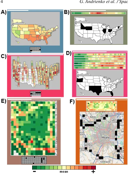
spa-Figure 1: Possible appearances of cells in a SOM matrix. Left: space-in-time SOM (grouping of spatial situations). Right: time-in-space SOM (grouping of places according to temporal variations of attribute values). A,B: one attribute with values for 41 years. C,D: 7 attributes with values for 41 years. E,F: one attribute with values for 7x24 hours. The upper image in each cell is the feature image, the lower im-age is the index imim-age.
tial, temporal, and thematic (attributive) components of the data.
3.2.1. Feature images
Feature imagesrepresent the objects to which the SOM tool has been applied, i.e. spatial situations in a space-in-time SOM and local temporal variations in a time-in-space SOM. Spatial situations are represented by maps (Figure1, left), and local temporal variations by diagrams (Figure1, right);
we call them ’temporal mosaics’. A map image portrays
the attribute values attained in all places in one time unit. A temporal mosaic portrays the attribute values attained in one place in all time units. In both cases, values of space-and time-dependent numeric attributes are represented by color coding. The user may choose one of the multiple color scales available in the system, which include all variants of diverging color scales from Color Brewer [HB03]. Thus, in Figure1, a Color Brewer’s scale is used where shades of green correspond to low values, shades of red to high
val-ues, and yellow stands for values close to the average. In Figure2, a modified variant of one of the Color Brewer’s scales where color brightness is enhanced for more visual salience. Here, shades of blue are used for low values, shades of yellow for medium values, and shades of red for high val-ues. The system also includes some of the palettes suggested in [WVvWvdL08].
It should be noted that feature images are not meant for conveying detailed information about the values of attributes in each particular place and time unit. The system has other tools that enable detailed reading of values. For example, the cartographic map display not only allows the user to de-code the colors by means of the legend but also shows the exact values when the user points on a place in the map. The images in the SOM cells are intended for providing an overview, so that the user can approximately estimate whether the values are low, medium, or high and notice ma-jor differences between cells.
The cartographic representation technique used in the map images depends on the number of attributes selected for the analysis. Values of a single attribute are represented directly by colors of the map elements depicting the places (territory compartments). Examples can be seen in Figure
1A and E. In case of two or more attributes, the map con-tains diagrams, called’multi-attribute mosaics’, which are positioned in the places (Figure1C). Each diagram consists of pixels colored according to the attribute values and ar-ranged in a rectangular layout with user-preferred number of columns. Thus, in Figure1C, the multi-attribute mosaic in each compartment consists of 7 pixels arranged in one col-umn. The pixels correspond to 7 attributes selected for the analysis. Overlapping of the mosaic symbols on the small maps is a serious problem, which is only partly reduced by semi-transparent rendering. Still, the images are adequate for providing an overview: the user can see which colors prevail where.
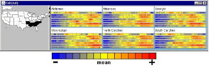
[image:5.595.71.288.66.361.2]G. Andrienko et al. / Space-in-time and time-in-space SOMs 5
Figure 2: An additional window displays the content of a cell of a time-in-space SOM.
7 rows. Although the resulting image is similar to that in Figure1F, the meaning of the rows is different.
In case of multiple attributes, the values of each attribute are color-coded independently of the other attributes while the same color scale is used. Since the same colors may rep-resent different value intervals for different attributes, fea-ture images are not meant to be used for inter-attribute com-parisons. Their role is to give an idea about the relative mag-nitudes of the individual attribute values.
When a SOM matrix cell contains two or more objects, the displayed image represents the best fitting object, that is, the object with the smallest distance to the cell’s prototype vector (nearest neighbor). Images of all objects included in a cell can be seen in an additional window which appears after clicking on the cell (Figure2).
3.2.2. Index images
Index imagesshow the temporal or spatial positions of the objects included in the SOM matrix cells. In a space-in-time SOM,temporal index imagesshow the temporal positions of the spatial situations (Figure1left). An image consists of small squares representing the time units, which are tem-porally ordered and arranged in rows of user-chosen length. The squares representing the objects included in the respec-tive SOM cell are filled in black. Thus, in Figure1A and B, the temporal index images have 10 columns; hence, the rows correspond to decades. In Figure1C, the temporal index im-age has 24 columns corresponding to 24 hours of a day and 7 rows corresponding to 7 consecutive days.
In a time-in-space SOM,spatial index imagesshow the
spatial positions of the local temporal variations. Each image is a map where the spatial positions are marked by black filling of the corresponding territory compartments (Figure1
right). The combination of feature images and index images provides a combined representation of the space, time, and values of one or more attributes. The user may arbitrarily switch on and off the drawing of the feature images and the index images.
3.2.3. Distances between SOM cells
In a SOM, not every single neuron necessarily represents a meaningful cluster. In many cases, it is useful to see a
com-bination of nearby neurons as representation for such a clus-ter. The u-matrix [Ult99], which consists of the pair-wise distances between neighboring cells in the space of the at-tribute values, is a common way to address this problem. In our implementation, the information about the distances may be conveyed in the SOM matrix display through the shading of the cell borders (Figure8). The border of a cell is divided into 8 segments corresponding to the 8 neighbors of this cell. The degree of darkness of each segment between white and black is proportional to the Euclidean distance to the respec-tive neighbor in terms of the attribute values. The distances among the SOM cells are also reflected in the coloring of the SOM cells, as explained below. Therefore, the drawing of the so shaded borders between the cells is optional and can be switched off by the user.
3.2.4. Coloring of SOM cells
Coloring of the cells in the SOM matrix is the primary means for visual linking of the matrix display to the other visual dis-plays and thus for putting SOM results in the spatial and tem-poral contexts. For this purpose, the colors of the cells are assigned to the spatial or temporal positions of the thereby represented objects and used for coloring the corresponding visual elements in the other displays. To enable correct per-ception of the similarities and dissimilarities from the dis-plays linked to SOM, the coloring of the SOM cells must re-flect the distances among them in the attribute values space.
To achieve this, we create for a SOM matrix with m
columns and n rows a two-dimensional color map with
10*m columns and 10*n rows. In the next step, we place
the first neuron in the corresponding corner of the color ma-trix. Then each next neuron is iteratively placed in the color matrix according to the distances to its previously placed neighbors. Using this strategy, neighboring cells with a small distance have more similar colors than cell pairs with a big distance, reflecting the actual data similarity. For a two-dimensional color map, we use the CIELab color space as suggested in [WD08].
4. Validation of the framework: detecting the expected
Figure 3: The space-in-time SOM matrix with the hourly traffic situations in Milan characterized in terms of the mean speeds in the spatial compartments.
each pair <place, time unit> we computed the mean speed of the movement. This attribute is adequate for character-izing traffic conditions. The mean speed is high when the conditions are favorable and low when the movement is ob-structed, e.g. because of traffic congestion. The data were previously cleaned so that the cars that did not move for 10 or more minutes were not taken into account. The combina-tions <place, time interval> in which there were no cars have got zero values of the mean speed.
Hence, the spatial situation in each time unit is character-ized by the mean speeds in all places. The local temporal variation in each place is characterized by the time series of the mean speeds in this place.
4.1. Detection of temporal patterns among spatial situations
The typical temporal patterns of traffic situations in a big city are well known. Thus, there are particular intervals in the mornings of the working days, called "rush hours", when the major streets are crowded with vehicles and the movement is obstructed. Similar situations occur in the afternoons. Be-tween these intervals, the situation may improve but the movement is not as free as in late evenings and nights. The patterns on weekends and holidays are usually quite differ-ent. Situations with heavily obstructed traffic either do not occur or occur in other time intervals. If shops are closed on Sundays, differences between Sunday and Saturday patterns can be expected. We tried to detect these expected temporal patterns by grouping similar spatial situations with the help of SOM.
Figure 4: The Time Arranger exposes periodic temporal patterns in the evolution of the traffic situation in Milan over the week. The columns correspond to the 24 hourly intervals of a day and the rows to the 7 days from Sunday to Saturday. The pixels have the colors of the SOM cells (Figure3) in which the respective time units belong.
We ran SOM with the following parameters: matrix size 5x3, 300,000 iterations, learning radius 2, learning rate 0.02. The resulting space-in-time SOM matrix is shown in Figure
3. As mentioned before, cell colors in a SOM matrix link it to other displays. Colors from a space-in-time SOM can be transmitted, in particular, to a time arranger display (Fig-ure4). It consists of rectangular pixels representing the time units and having the colors of the SOM cells the units be-long in. The pixels are chronologically ordered and arranged in rows. By choosing suitable row length and indention of the first row, the user can detect periodic temporal patterns in the occurrence of the spatial situations. Periodicity is man-ifested by vertical alignments of identically or similarly col-ored pixels. Thus, the pixels in Figure4represent hourly in-tervals within a 7-day period from Sunday to Saturday. They are arranged in rows of the length 24, which corresponds to 24 hours of a day. The prominent vertical alignments of similarly colored pixels mean that the spatial situations were similar in the corresponding hours of different days. It is easy to see that Sunday (first row) and Saturday (last row) differ from the working days. Friday morning is similar to the mornings of the other working days while the color pat-tern of the rest of the day is more similar to that on Saturday. We found out that this was not a typical working Friday but the Good Friday before Easter, which may explain the dif-ference.
[image:7.595.337.502.81.200.2]G. Andrienko et al. / Space-in-time and time-in-space SOMs 7
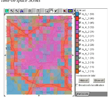
Figure 5:The time-in-space SOM matrix with the local tem-poral variations of the mean speeds in the spatial compart-ments in Milan.
from the interval 5-6AM, the pixels are colored in light blue, which corresponds to the upper right corner of the matrix. The speeds are low almost throughout the whole city. Very close to that are the situations in the middle right cell of the matrix (light violet); only on the west and south of the city the speeds are somewhat higher. Apparently, the inter-val 5-6AM is the beginning of the rush hours, which last till 10AM from Monday to Wednesday and on Friday and till 18 o’clock on Tuesday. From Monday to Wednesday, the obstructed traffic situations repeat from 15 to 17 o’clock. Be-tween and after the rush hours the speeds are higher mainly on the major roads (lower right corner of the matrix). In the evening (from about 20 o’clock), the speeds increase also in other parts of the city (lower left corner).
Hence, we can conclude that our tools allowed us to detect the expected periodic temporal patterns in the weekly traffic in Milan. Periodicity in time-dependent data can also be re-vealed using other arrangements of display elements; thus, in [SDW08], a diagonal arrangement is used.
4.2. Detection of spatial patterns among local temporal variations
[image:8.595.72.289.79.273.2]An obvious spatial pattern that can be expected in the dis-tribution of the local temporal variations is that the traffic on the major roads differs from that in the city center. One can also expect a different profile of the traffic variation in residential areas. To detect such patterns, we group the local temporal variations with the help of SOM using the same pa-rameters as in the previous experiment. The resulting time-in-space SOM matrix is shown in Figure5. In Figure6, the colors of the SOM cells are used for painting the places on
Figure 6: The map of Milan with the places colored as the cells of the time-in-space SOM (Figure5) they belong in.
the map of Milan. The places on the major roads are colored mostly in red, which clearly differentiates them from the re-maining territory. The speeds in these places are high except for the rush hours (see the temporal mosaics in the lower left corner of the matrix). The places in the city center are col-ored in pink. Here the speeds are always quite low. Shades of light blue are in places with little or no movement (many of the mean speed values are zeros). It is highly probable that they are in pedestrian or residential areas. Hence, we can say that our tools, indeed, enabled us to detect the expected spatial patterns. We also noticed something unexpected: the speeds on the belt road on the northeast are much lower than typically on the belt roads (see cell 2,2 of the matrix).
5. Application of the framework: discovering the unexpected
In this experiment, we apply our framework to the USA crime dataset published by the US Department of Justice. We downloaded the data from the URL http://bjsdata.ojp.usdoj.gov/dataonline/ in March 2003. For 50 states of the USA plus District of Columbia, there are annual statistics for the years from 1960 to 2000 including the rates of seven types of crime: Murder and non-negligent manslaughter, Forcible rape, Robbery, Aggravated assault, Burglary, Larceny-theft, and Motor vehicle theft. We want to explore the spatial and temporal patterns of these crime rates. Before starting the analysis, we look at the variation of the values of the attributes using a time graph display (Figure
Figure 7: A fragment of the time graph display of the tem-poral variations of the crime rates.
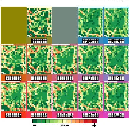
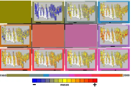
Figure 8:The space-in-time SOM matrix of the yearly crime situations in the USA.
to make the values in the states more comparable, we trans-form the original data into differences from the states’ mean values divided by the respective standard deviations. For this purpose, we use the interactive interface for data transforma-tion integrated in the time graph display. Figure9A shows the result for 4 out of 7 attributes. From now on, we use the transformed data.
5.1. Discovery of temporal patterns among spatial situations
To investigate how the spatial distribution of the crime rates values evolves over time, we apply SOM to the spatial situ-ations in the years from 1960 to 2000 where each situation is characterized by the values of the seven crime rates. We use the following parameters: matrix size 4x3, 200,000 it-erations, learning radius 2, learning rate 0.02. The resulting space-in-time SOM is shown in Figure8. In this case, we used a color scale with enhanced brightness for the color coding of the attribute values in order to increase the visibil-ity of the semi-transparent symbols on the maps. Below the matrix, Figure8shows a fragment of the time arranger dis-play where the pixels are arranged in one row and have the colors of the respective SOM cells. The pixels in the index images are also arranged in one row. It is well visible that
Figure 9: A) A fragment of the time graph display where the original data have been transformed to normalized dif-ferences from the mean values. The background painting of the time intervals uses the cell colors from the space-in-time SOM in Figure8. B) The data have been further transformed to the differences with respect to the previous years. Instead of the lines of the individual states, the 0th, 20th, 40th, 60th, 80th, and 100th percentiles in each year are indicated by the vertical positions of the edges of the alternating stripes with lighter and darker shading, as suggested in [AA05a].
the period 1960-2000 has been divided into continuous in-tervals. The way in which the colors change from interval to interval indicate gradual or abrupt changes of the crime sit-uations. From the feature images in the matrix it is clear that the crime rates were low in the initial interval and then in-creased reaching maximums in 1975-1981. After that, there was some decrease in 1982-1983 and 1984-1989 and then increase during the following intervals but without reaching such extreme values as in 1975-1981. In 2000, many of the values go down again.
In Figure9A the colors of the SOM cells have been trans-mitted to the time graph display. To understand better the character of the changes from one interval to another, we do a further data transformation in the time graph display: the values in each year are replaced by the differences w.r.t. the previous year. In Figure9B the differences are represented in a summarized form as suggested in [AA05a]. The verti-cal lines mark 1973 as a year of substantial change, judg-ing from the remarkable color assigned to the interval 1973-1974. We can see that the burglary and robbery rates (and the larceny-theft rate, which is not shown in Figure9) highly in-creased in 1974 in at least 80% states.
[image:9.595.73.289.223.369.2]G. Andrienko et al. / Space-in-time and time-in-space SOMs 9
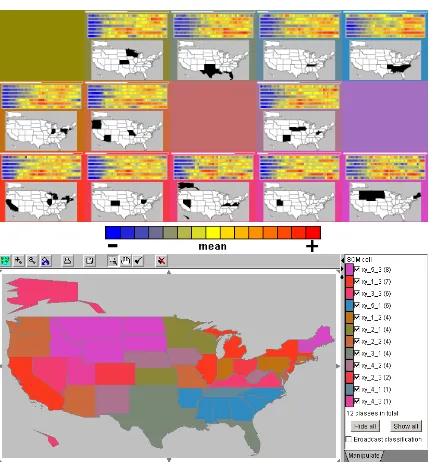
Figure 10: Top: the time-in-space SOM matrix grouping and arranging the states of the USA according to the tempo-ral variations of the values of 7 crime attributes. Bottom: the map of the USA with the states painted in the colors of the matrix cells.
of the states. However, this is not the only possible type of situation change; thus, it seems that the change in 1968 was not of this kind. We additionally look at an animated map display presenting the values of the seven attributes. Like the time graph, the map display allows us to transform the values into the differences with respect to previous years, so that we can see where the values substantially increased or decreased. For instance, in 1968 four out of the seven crime rates highly increased on the northwest of the USA.
5.2. Discovery of spatial patterns among local temporal variations
Now we apply the SOM to the local temporal variations in the states using the parameters: matrix size 5x3, 200,000 it-erations, learning radius 2, learning rate 0.02. We use the index images in the SOM cells and the SOM-linked map dis-play (Figure10) to see how the states with similar temporal variations are distributed in space. There are several spatial clusters formed by neighboring states with identical or simi-lar coloring. Some states are not very simisimi-lar to their neigh-bors; thus, California is more similar to the states near the Great Lakes. The group of states on the southeast, evidently, differs greatly from the states on the northeast, as indicated by a sharp difference in the colors. The commonalities and differences among the states can be understood by inspect-ing the feature images and by transmittinspect-ing the groupinspect-ing and
colors of the states to the time graph display, as described in [AA05b]. Thus, we found that the values of all crime rates except the first one (murders) in the southeastern states (see Figure2) mostly increased during the period 1960-2000 and reached their maximums an the last decade. The variation pattern in the other states is different: the highest values were achieved in the middle of the period (around 1975-1985) but than decreased. Only the group of states Texas, Okla-homa, Louisiana, and Florida (middle top cell of the matrix) is somewhat similar to the southeastern states in terms of the temporal variation patterns.
6. Discussion and conclusion
We have demonstrated how our tools, which combine in-teractive visual interfaces with the computational SOM method, enable comprehensive exploration of multivariate spatiotemporal data and discovery of high-level patterns. Al-though SOM has been previously applied to spatial, tempo-ral, and spatiotemporal data, our framework uses this method in a novel way. Our main innovation with respect to the state of the art is the support of two complementary an-alytic tasks based on two perspectives of spatiotemporal data: as spatial situations changing over time and as tem-poral variation profiles distributed over space. To the best of our knowledge, there are no analogues to our framework in the literature. Previously, SOM has been applied to com-binations of attribute values describing pairs <place + time unit> [GCML06]. We apply SOM to higher level constructs, namely, spatial situations and local temporal variations. As a result, the outcomes of the method match the two high-level analysis subtasks much more closely than in the previous approaches.
We have also developed innovative ways to visualize SOM outcomes. While propagating cell colors from SOM to other displays is a common approach, we use special color scales reflecting the similarity among the cells. We put fea-ture images and index images in SOM matrix cells to give a combined representation of the spatial, temporal, and at-tributive (thematic) components of the data and thereby fa-cilitate understanding of the SOM outcomes. The coordi-nated spatial and temporal displays with integrated tools for interactive visually-supported data transformations help in preparing data to the application of SOM and in interpreting its results.
7. Acknowledgments
[image:10.595.73.288.77.309.2]References
[AA05a] ANDRIENKOG. L., ANDRIENKON. V.: Visual ex-ploration of the spatial distribution of temporal behaviors. In
9th International Conference on Information Visualisation, IV 2005, 6-8 July 2005, London, UK(2005), IEEE Computer So-ciety, pp. 799–806.8
[AA05b] ANDRIENKON., ANDRIENKOG.: Exploratory Anal-ysis of Spatial and Temporal Data: A Systematic Approach. Springer-Verlag, 2005.2,9
[AA08] ANDRIENKOG., ANDRIENKON.: Spatio-temporal ag-gregation for visual analysis of movements. InVisual Analytics Science and Technology, 2008. VAST ’08. IEEE Symposium on
(Oct. 2008), pp. 51–58.5
[AAD∗08] ANDRIENKOG., ANDRIENKON., DYKESJ., FAB
-RIKANTS. I., WACHOWICZM.: Geovisualization of dynamics, movement and change: key issues and developing approaches in visualization research. Information Visualization 7, 3/4 (2008), 173–180.http://dx.doi.org/10.1057/ivs.2008.23.1
[AS08] AGARWALP., SKUPINA. (Eds.):Self-Organising Maps: Applications in Geographic Information Science. Wiley, 2008.2
[Bar08] BARTHELK. U.: Improved image retrieval using au-tomatic image sorting and semi-auau-tomatic generation of image semantics. Image Analysis for Multimedia Interactive Services, International Workshop on 0(2008), 227–230.2
[BLP05] BAÇÃOF., LOBOV., PAINHOM.: The self-organizing map, the geo-som, and relevant variants for geosciences. Com-puters & Geosciences 31, 2 (2005), 155 – 163. Geospatial Re-search in Europe: AGILE 2003.2
[DK98] DEBOECKG., KOHONENT. (Eds.):Visual Explorations in Finance: with Self-Organizing Maps. Springer, 1998.2
[GCML06] GUOD., CHENJ., MACEACHRENA. M., LIAOK.: A visualization system for space-time and multivariate patterns (VIS-STAMP). IEEE Transactions on Visualization and Com-puter Graphics 12, 6 (2006), 1461–1474.2,3,9
[GGM∗05] GUOD., GAHEGANM., MACEACHRENA., , ZHOU
B.: Multivariate analysis and geovisualization with an integrated geographic knowledge discovery approach. Cartography and Geographic Information Science 32, 2 (2005), 113–132.2
[HB03] HARROWERM., BREWERC. A.: Colorbrewer.org: An online tool for selecting colour schemes for maps. The Carto-graphic Journal 40, 1 (2003), 27–37.4
[Hew08] HEWITSONB. C.: Climate analysis, modelling, and regional downscaling using self-organizing maps. In Self-Organising Maps: Applications in Geographic Information Sci-ence, Agarwal P., Skupin A., (Eds.). Wiley, 2008, pp. 137–163.
2
[KHKL96] KOHONENT., HYNNINENJ., KANGASJ., LAAKSO
-NENJ.:SOM_PAK: The Self-Organizing Map Program Package. Tech. Rep. A31, Helsinki University of Technology, 1996.3
[KK08] KOUAE. L., KRAAKM.-J.: An integrated exploratory geovisualization environment based on self-organizing map. In
Self-Organising Maps: Applications in Geographic Information Science, Agarwal P., Skupin A., (Eds.). Wiley, 2008, pp. 45–66.
2
[Koh01] KOHONENT.:Self-Organizing Maps. Springer-Verlag, 2001.2,3
[KVK00] KASKIS., VENNAJ., KOHONENT.: Coloring that re-veals cluster structures in multivariate data. InAustralian Journal of Intelligent Information Processing Systems(2000), pp. 6–82.
2
[ND06] NUERNBERGERA., DETYNIECKIM.: Externally grow-ing self-organizgrow-ing maps and its application to e-mail database visualization and exploration. Applied Soft Computing 6, 4 (2006), 357–371.2
[Peu02] PEUQUETD. J.:Representations of Space and Time. The Guilford Press, 2002.1
[SBvLK09] SCHRECKT., BERNARDJ.,VONLANDESBERGER
T., KOHLHAMMERJ.: Visual cluster analysis of trajectory data with interactive kohonen maps. Information Visualization 8, 1 (2009), 14–29.2
[SDW08] SLINGSBYA., DYKESJ., WOODJ.: Using treemaps for variable selection in spatio-temporal visualization. Informa-tion VisualizaInforma-tion 7, 3-4 (2008), 210–224.7
[Sku08] SKUPINA.: Visualizing human movement in attribute space. InSelf-Organising Maps: Applications in Geographic In-formation Science, Agarwal P., Skupin A., (Eds.). Wiley, 2008, pp. 121–135.2
[ST08] SPIELMANS. E., THILLJ.-C.: Social area analysis, data mining, and gis. Computers, Environment and Urban Systems 32, 2 (2008), 110–122.2
[Ult99] ULTSCHA.: Data mining and knowledge discovery with emergent self-organizing feature maps for multivariate time se-ries. InKohonen Maps(1999), Elsevier, pp. 33–46.5
[Ves99] VESANTO J.: SOM-based data visualization methods.
Intelligent Data Analysis 3, 2 (1999), 111–126.2
[WD08] WOODJ., DYKESJ.: Spatially ordered treemaps.IEEE Trans. Vis. Comput. Graph. 14, 6 (2008), 1348–1355.5
[WVvWvdL08] WIJFFELAARS M., VLIEGEN R., VAN WIJK