The problems of assessing software reliability ...When you really need to depend on it

      

City, University of London Institutional Repository

Citation

:

Littlewood, B. (2000). The problems of assessing software reliability ...When you really need to depend on it. Paper presented at the Conference on Lessons in System Safety.

This is the unspecified version of the paper.

This version of the publication may differ from the final published

version.

Permanent repository link:

http://openaccess.city.ac.uk/1632/

Link to published version

:

Copyright and reuse:

City Research Online aims to make research

outputs of City, University of London available to a wider audience.

Copyright and Moral Rights remain with the author(s) and/or copyright

holders. URLs from City Research Online may be freely distributed and

linked to.

City Research Online: http://openaccess.city.ac.uk/ [email protected]

The Problems of Assessing Software Reliability

....when you really need to depend on it

Bev Littlewood

Centre for Software Reliability, City University London, UK

Abstract

This paper looks at the ways in which the reliability of software can be assessed and predicted. It shows that the levels of reliability that can be claimed with scientific justification are relatively modest

1

Introduction

The question of how safe a critical system needs to be is ultimately determined by what is regarded as an acceptable risk to society (usually as judged by its agents, such as regulators). It will involve an analysis of benefits and costs, particularly those associated with safety-related failures. See, for example, [HSE 1992] for an interesting and accessible discussion of this problem in the context of the safety of nuclear power stations.

Making a system acceptably safe, and demonstrating that this is so, is an

engineering task. This paper addresses the last of these problems; more specifically it is concerned with the difficult job of assessing the contribution that software makes to the safety of a wider system.

Software is now ubiquitous in engineered systems, including safety-critical ones. Not only is it used to replace older, well-understood technologies, it is more and more frequently used to implement completely novel functionality. Some of these new applications (e.g. flight-critical control of unstable aircraft) pose very difficult problems to system designers, and result in considerable design complexity. Novelty, difficulty and complexity tend to militate against reliability of software, and of course this can become a threat to the safety of the overall system.

Reliability requirements for software will depend upon a safety analysis of the wider system of which the software is a part. Not only will the required levels vary from one application to another, but the nature of the reliability claims can differ. In a safety system, such as a nuclear reactor protection system, the requirement might be expressed as a probability of failure on demand (in the case of the software-based Sizewell B Primary Protection System, the requirement was 10-3 pfd). In a continuous control system, for example in aircraft flight control, the reliability requirement might be expressed as a failure rate (e.g. 10-9 probability of failure per flight hour). In some cases there may, in addition, be a requirement to meet an

availability goal (e.g. the requirement for the US AAS air traffic control system was

Some of these reliability levels are extremely demanding - a figure of 10-12 probability of failure per hour has been mentioned in relation to some railway applications. Is it possible to assess reliabilities at these levels with sufficient scientific rigour to satisfy the needs of wider system safety cases? In the main part of the paper this question will be addressed in some detail, identifying the limits to the levels of reliability that can be claimed before a system has been exposed to extensive operational use.

Before coming to this, however, it may be useful to address briefly some misconceptions about the nature of software reliability, and in particular to show the inevitability of a probabilistic approach.

2

The nature of the software failure process

The distinction that is made in reliability engineering between random

failures (meaning, usually, conventional hardware failures) and systematic failures

(e.g. failures arising from design faults, usually - but not necessarily - from software) is very misleading. This terminology appears to suggest that in the former case a probabilistic approach is inevitable, because of the ‘randomness’, but that in the latter it is possible to get away with completely deterministic arguments. In fact this is not the case, and probabilistic arguments seem inevitable in both cases.

The use of the word systematic here refers to the fault mechanism, i.e. the mechanism whereby a fault reveals itself as a failure, and not to the failure process. Thus it is correct to say that if a fault of this class has shown itself in certain circumstances, then it can be guaranteed to show itself whenever these circumstances are exactly reproduced. In the terminology of software, which is usually considered the most important source of systematic failures, it is right say that if a program failed once on a particular input case it would always fail on that input case until the offending fault had been successfully removed. In this sense there is determinism, and it is from this determinism that we obtain the terminology1

.

In fact, of course, interest really centres upon the failure process: what is seen when the system under study is used in its operational environment. There is natural uncertainty in this process, arising from the nature of the operational environment. Specifically, there is uncertainty as to when a member of the set of input cases that trigger a particular fault will next occur. Thus there is uncertainty as to when the next failure of the program will occur. This forces the use of probabilistic measures of reliability even for ‘systematic’ failures.

The important point is that the failure processes are not deterministic for either ‘systematic’ faults or for random faults. The same probabilistic measures of reliability are appropriate in both cases (although the details of the probability models for evaluating software reliability generally differ from those used for hardware [Lyu 1996]).

1

3

Reliability evaluation based on operational

testing

The only ways of directly measuring reliability require that we see the system running in an operational environment. The observed frequency of failures after a certain amount of exposure to this kind of testing (or the absence of failure) allows reliability estimates to be computed using statistical models.

Clearly, the difficulty of constructing a test regime that accurately captures all the relevant features of the actual operational environment will vary from one application domain to another. In some industries accurate simulation of operation has been possible for a long time: examples include the aircraft (flight-critical avionics) and nuclear industries (e.g. the extensive statistical testing used to evaluate the reliability of the Sizewell B PPS software after licensing [May, Hughes et al. 1995]).

The techniques for predicting future reliability from observed behaviour can be divided into two categories, dealing with two different forms of the prediction problem:

•

steady-state reliability estimation uses the results of testing the version of

the software that is to be deployed for operational use (‘as delivered’); the theory underlying this prediction is much the same as used in predicting the reliability of physical objects from sample testing;

•

reliability growth-based prediction uses the series of successive versions of

the software that are created, tested, and corrected after tests discover faults, leading to the final version of the software that is to be evaluated. The data used in this case are the results (series of successful and of failed tests) of testing each successive version. Having observed a trend of (usually) increasing reliability, this trend can be extrapolated into the future.

Steady-state evaluation is the more straightforward procedure, and requires

fewer assumptions. The behaviour of the system in the past is seen as a sample from the space of its possible behaviours. The aspect of interest of this behaviour, i.e., the occurrence of failures, is governed by parameters (typically, a failure rate or a probability of failure per demand) that can be estimated via standard inference techniques. Many projects, however, budget for little or no operational testing of a completed design before its deployment, or reliability requirements are set higher than their budgeted amount of testing can confirm with the required confidence. Reliability growth-based prediction is then an appealing alternative, because it allows the assessor to use the evidence accumulated while the product was ‘debugged’ rather than just evidence about its final version. However, any prediction depends on trusting that the trend will continue. In a macroscopic sense, this requires that no qualitative change in the debugging process interrupts the trend (e.g., a change of the debugging team, or the integration of new functionalities could bring about such a change). It also requires trust that the very last fix to the software was not an ‘unlucky’ one, which decreased reliability: this is particularly relevant in the case of safety-related systems.

necessary that the test case selection mechanism produces cases that are statistically representative of those that present themselves during operational use. This is not always easy, but there is a good understanding of appropriate techniques, as well as some experience of it being carried out in realistic industrial conditions, with the test-based predictions being validated by observation of later operational use [Dyer 1992; Musa 1993].

It is also worth emphasising that, although we often speak loosely of the reliability of a software product, in fact we really mean the reliability of the product

working in a particular environment, since the perceived reliability might vary

considerably from one user to another. It is a truism, for example, that operating system reliability can differ greatly from one site to another. It is not currently possible to test a program in one environment (i.e., with a given selection of test cases) and use the reliability modelling techniques to predict how reliable it will be in another.

3 . 1

Reliability growth assessment and prediction

Reliability growth models are statistical techniques that allow the direct evaluation of the reliability of a software product from observation of its actual failure process during operation. In their simplest form, it is assumed that when a failure occurs there is an attempt to identify and remove the design fault which caused the failure, whereupon the software is set running again, eventually to fail once again. The successive times of failure-free working are the input to statistical models, which use this data to estimate the current reliability of the program under study, and to predict how the reliability will change in the future.

There is an extensive literature on reliability growth modelling, with many detailed probability models purporting to represent the probabilistic failure process. Unfortunately, there is no single model that can be trusted to give accurate results in all circumstances, nor is there any way in which the most suitable model can be chosen a priori for a particular situation. In recent years, however, this difficulty has largely been overcome by the provision of methods for analysing the predictive accuracy of different models on a particular source of failure data [Abdel-Ghaly, Chan et al. 1986; Brocklehurst and Littlewood 1992; Lyu 1996]. The result is that we can now apply many of the available models to the failure data coming from a particular product, and gradually learn which (if any) of the different predictions can be trusted.

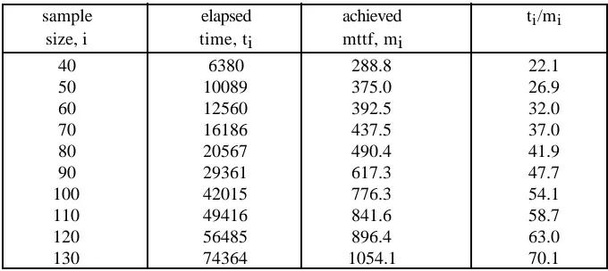
With the reservations stated above about the need for a statistically representative test regime, it is now possible to obtain accurate reliability predictions for software in many cases and, perhaps equally importantly, to know when particular predictions can be trusted. Unfortunately it seems clear that such methods are really only suitable for the assurance of relatively modest reliability goals. This can be seen by considering the following examples.

final column shows a clear law of diminishing returns: later improvements in the

mttf require proportionally longer testing.

sample elapsed achieved ti/mi

size, i _{time, ti mttf, mi}

40 6380 288.8 22.1

50 10089 375.0 26.9

60 12560 392.5 32.0

70 16186 437.5 37.0

80 20567 490.4 41.9

90 29361 617.3 47.7

100 42015 776.3 54.1

110 49416 841.6 58.7

120 56485 896.4 63.0

[image:6.612.121.461.113.265.2]

130 74364 1054.1 70.1

Table 1 An illustration of the law of diminishing returns in

heroic debugging. Here the total execution time (seconds) required to reach a particular mean time to failure is compared with the mean itself.

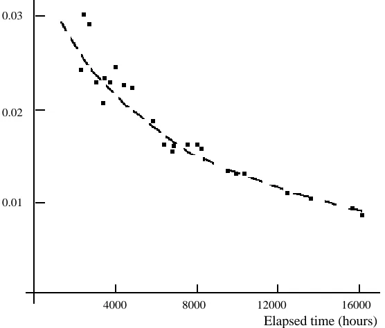
Of course, this is only a single piece of evidence, involving a particular measure of reliability (mttf), and the use of a particular model to perform the calculations, and a particular program under study. However, similar results are observed consistently across different data sources and for different reliability growth models. Figure 2 shows an analysis of failure data from a system in operational use, for which software and hardware design changes were being introduced as a result of the failures. Here the current rate of occurrence of failures (ROCOF) is computed at various times, using a different reliability growth model from that used in Table 1. The dotted line is fitted manually to give a visual impression of what, again, seems to be a very clear law of diminishing returns. Once again, the level of reliability reached here is quite modest: about 10-2 failures per hour of operational use, which is several orders of magnitude short of what we could call ‘ultra-high dependability’ (compare it with the 10–9 per hour requirement of the civil aircraft flight control systems). More importantly, it is by no means obvious how the details of the future reliability growth of this system will look. For example, it is not clear to what the curve is asymptotic: could one expect that eventually the ROCOF will approach zero, or is there an irreducible level of residual unreliability reached when the effects of correct fault removal are balanced by those of new fault insertion?

This empirical evidence of a law of diminishing returns for debugging software, shown by these two examples, seems to be supported by most of the available evidence. Certainly it is a feature of all the data sets that have been analysed within the Centre for Software Reliability. There are convincing intuitive reasons for results of this kind.

overall unreliability of the program: some are ‘larger’ than others. ‘Large’ here means that the rate at which the fault would show itself (i.e. if we were not to remove it the first time we saw it) is large: different faults have different rates of occurrence. Table 2 shows a particularly dramatic example of this based on a large database of problem reports for some large IBM systems [Adams 1984].

4000 8000 12000 16000

0.01 0.02 0.03

Elapsed time (hours)

F i g u r e 2 Estimates of the rate of occurrence of failures for a

system experiencing failures due to software faults and hardware design faults. The broken line here is fitted by eye. Once again, the rate is not recomputed at each data point here: the plotted points represent only occasional recomputation of the rate during the observation of several hundred failures.

During reliability growth we assume that a fix is carried out at each failure. Let us assume for simplicity that each fix attempt is successful (this assumption, whilst thoroughly unrealistic, does not affect the general thrust of the present argument). As debugging progresses, there will be a tendency for a fault with a larger rate to show itself before a fault with a smaller rate: more precisely, for any time t, the probability that fault A reveals itself during time t will be smaller than the probability that B reveals itself during t, if the rate of A is smaller than the rate of B. Informally, large faults get removed earlier than small ones. It follows that the improvements in the reliability of the program due to earlier fixes, corresponding to faults which are likely to be larger, are greater than those due to later fixes.

[image:7.612.150.428.140.377.2]

program is failing is becoming smaller), and the improvements to the reliability

resulting from these fault-removals are also becoming smaller and smaller.

R a t e C l a s s

1 2 3 4 5 6 7 8

Mean time to occurrence in kmonths for rate class

60 19 6 1.9 .6 .19 .06 .019

Product Estimated percentage of faults in rate class

1 34.2 28.8 17.8 10.3 5.0 2.1 1.2 0.7

2 34.3 29.0 18.2 9.7 4.5 3.2 1.5 0.7

3 33.7 28.5 18.0 8.7 6.5 2.8 1.4 0.4

4 34.2 28.5 18.7 11.9 4.4 2.0 0.3 0.1

5 34.2 28.5 18.4 9.4 4.4 2.9 1.4 0.7

6 32.0 28.2 20.1 11.5 5.0 2.1 0.8 0.3

7 34.0 28.5 18.5 9.9 4.5 2.7 1.4 0.6

8 31.9 27.1 18.4 11.1 6.5 2.7 1.4 1.1

[image:8.612.126.463.116.317.2]

9 31.2 27.6 20.4 12.8 5.6 1.9 0.5 0.0

Table 2 Data from [Adams 1984], showing the very

great disparity in ‘sizes’ of software faults. Here size is taken to be the mean time it would take to discover a fault (or alternatively its reciprocal, the rate of occurrence of the fault). Adams classified the faults into eight classes according to their sizes, and the most notable aspect of the above figures is the very large differences between the ‘largest’ and the ‘smallest’. Perhaps most startling is that about one third of faults fall into the 60 kmonth class: i.e. a fault from this class would only be seen at the rate of about once every 5000 years!

3 . 2

Reliability estimation based on failure-free working

In the discussion above, there has been an important implicit assumption that it is possible to fix a fault when it has been revealed during the test, and to

know that the fix is successful. In fact, there has been no serious attempt to model

The difficulty here is that the potential increase in unreliability due to a bad fix is unbounded. The history prior to the last failure, at least as this is used in current models, does not tell us anything about the effect of this last fix. Of course, in principle we could learn about the efficacy of previous fixes (although this would not be easy), and attempt to estimate the proportion of previous bad fixes. Thus we might take this proportion to be a good estimate of the probability that the current fix is a bad one. But in order to have high confidence that the reliability was even as high as it was immediately prior to the last failure, it would be necessary to have high confidence that no new fault had been introduced. There seem to be no good grounds to have such high confidence associated with a particular fix other than to exercise the software for a long time and never see a failure arise from the fix.

This seems to be the most serious objection to the use of software reliability growth models for the assessment of the reliability of safety-critical software, and it applies whatever the required level of reliability. Thus for nuclear safety systems, it is probably more serious even than the practical objection discussed above concerning the law of diminishing returns - after all, these nuclear systems have fairly modest reliability requirements, and it may be possible to test them for long sequences of demands. But even if it were practicable to use a reliability growth model to obtain an estimate of reliability of the order of 10-4 pfd, say, there would remain this residual doubt that the last fix(es) had introduced new sources of unreliability, rendering untrustworthy any estimate based on an extrapolation of earlier growth.

The conservative way forward in this case would be to treat the program following a fix as if it were a new program, and thus take into account only the period of failufree working that has been experienced since the last fix. This re-casts the problem in terms of steady-state reliability assessment. This problem has been studied in some detail in recent years [Littlewood and Strigini 1993; Littlewood and Wright 1997] but, not surprisingly, it turns out that the claims that can be made for the reliability of a system that has worked without failure are fairly modest for feasible periods of observation. Thus, in the case of a demand-based system such as a protection system, if we require to have 99% confidence that the pfd is no worse than 10-3, we must see about 4600 failure-free demands; for 99% confidence in 10-4, the number increases to 46000 failure-free demands: such a test was conducted for the Sizewell PPS [May, Hughes et al. 1995]. In the case of a continuously operating system, such as a control system, a 99% confidence in an MTTF of 104 hours (1.14 years) would require approximately 46,000 hours of failure-free testing; to raise the confidence bound on the MTTF to 105 hours, the testing duration must also increase to approximately 460,000 hours. In summary, high confidence in long failure-free operation in the future requires observing much longer failure-free operation under test. If this amount of test effort is not feasible, only much lower confidence can be obtained. For instance, it can be shown [Littlewood and Strigini 1993] via a simple Bayesian argument that, after seeing a system operating failure-free for t0 hours, one can only claim that it has a 50:50 chance of surviving for a further t0 hours before it

4

Indirect ways of evaluating software

reliability

There are clearly severe limitations to the levels of reliability that can be demonstrated using the direct evaluation approach, based on statistical analysis of operational testing data. Can this problem be overcome by using some other means of assessment? There seem to be three main candidates: claims based on quality of production, fault tolerance, and formal verification.

4 . 1

Reliability claims based on process quality

It seems to be assumed, in some industries, not only that the use of sufficiently good design and development practices can achieve very high reliability, but that the mere fact of their use guarantees that these levels will be met. For example, in [RTCA 1992] there is the statement:

‘ . . techniques for estimating the post-verification probabilities of software errors were examined. The objective was to develop numerical requirements for such probabilities for digital computer-based equipment and systems certification. The conclusion reached, however, was that currently available methods do not yield results in which confidence can be placed to the level required for this purpose. Accordingly, this document does not state post-verification software error requirements in these terms.’

The reader of these guidelines can only assume that the procedures and practices that are recommended in the document are somehow sufficient to justify reliability claims at the levels needed (10-9 probability of failure per hour for flight critical avionics!) without the need for direct measurement. Whilst no-one would deny that good practice is necessary for the development of extremely reliable safety-critical software, there is no evidence that it is sufficient.

The difficulty in claiming any reliability level for a program merely from evidence of the quality of its development process stem from two sources. In the first place, there is surprisingly little empirical evidence available of the operational reliability for software developed using particular development processes. Secondly, even if extensive evidence were available for a particular process, it would merely concern the reliability that might be expected on average. The actual achieved reliabilities would vary from one development to another, and thus there would be uncertainty involved in any reliability claim for a new product.

4 . 2

Fault tolerance based on design diversity

In hardware reliability engineering it is sometimes assumed that the stochastic failure processes of the different components in a parallel configuration are

independent. It is then easy to show that a system of arbitrarily high reliability can

be constructed by using sufficiently many unreliable components.

individual versions (these could be based on the techniques for direct evaluation described above).

Unfortunately, experiments show that design-diverse versions do not fail independently of one another [Knight and Leveson 1986b]. One reason for this is simply that the designers of the different versions tend to make similar mistakes. Another reason is more subtle [Eckhardt and Lee 1985; Littlewood and Miller 1989]: even if the different versions really are independent objects (defined in a plausible, precise fashion), they will still fail dependently as a result of variation of the ‘intrinsic hardness’ of the problem from one input case to another. Put simply, the failure of version A on a particular input suggests that this is a ‘difficult’ input, and thus the probability that version B will also fail on the same input is greater than it otherwise would be. The greater this variation of ‘difficulty’ over the input space, the greater will be the dependence in the observed failure behaviour of versions, and consequently the smaller the benefit gained from the diversity.

On the other hand, the experiments [Anderson, Barrett et al. 1985; Knight and Leveson 1986a] agree that fault tolerance brings some increase in reliability compared with single versions - the problem is knowing how much in a particular case. If independence of failure behaviour cannot be assumed, reliability models for fault-tolerant software require that the degree of dependence must be estimated in each case. Trying to do this using the operational behaviour of the system simply leads to the same infeasible ‘black-box’ estimation problem encountered earlier. There do not appear to be any other convincing procedures.

4 . 3

Formal verification

It is tempting to try to move away from probability-based notions of software reliability towards deterministic, logical claims for complete perfection. Thus if a formal specification of the problem could be trusted, a proof that the program truly implemented that specification would be a guarantee that no failures could arise due to design faults in the implementation. It could be said that the product was ‘perfectly reliable’ with respect to such a class of failures. Whilst such an approach has its attractions, there are some problems.

In the first place, proofs are subject to error. This might be direct human error, in proofs by hand or with the aid of semiautomatic tools, and/or error by the proof-producing software in machine proof. In principle, one could assign a failure probability to proofs, and use this in a probabilistic analysis. However, such probabilities would be difficult to incorporate into a dependability evaluation: in the event that the proof were erroneous, we would not know anything about the true failure rate.

There are also practical difficulties. Although automated approaches to verification have advanced considerably, there are still stringent limits to the size and complexity of problems that can be addressed in this way.

5

Evaluating reliability using several evidence

sources

For real systems, claims for software reliability in safety cases are usually based upon many different kinds of evidence. For example, in the evaluation of the Sizewell PPS software the evidence came from the software production process, from extensive testing, from static analysis using MALPAS [Hunns and Wainwright 1991].

5 . 1

Expert judgement and BBNs

Combining such disparate evidence to make a judgement of the reliability of a program is difficult for two reasons. In the first place, it is often hard to know how much value to give to each strand of evidence. In the case of Sizewell, for example, whilst the MALPAS analysis was impressive in its scope (the largest exercise of its type ever attempted), it fell short of complete verification - indeed some of the more complex parts of the code defied analysis. Similarly, although the testing was intensive, the tests were not statistically representative of operational demands, so it was not possible to make direct reliability claims, in the ways discussed earlier.

Secondly, the very disparate nature of the different evidence strands makes their combination difficult. In particular, it is often hard to tell how dependent they are: if we have seen a large and successful test run, how much should our confidence increase when, in addition, we learn that extensive static analysis has revealed no problems?

Currently, answers to questions like this are provided quite informally by human experts. In the example of the Sizewell PPS, interestingly, the consensus was that the evidence did not support a claim for the originally required reliability of 10-4 pfd, but was sufficient to claim 10-3 (which turned out to be small enough, following a re-examination of the wider plant safety case).

There is considerable research going on to help the expert with these problems. One promising formalism for combining evidence in the face of uncertainty is Bayesian Belief Nets (BBNs) [Fenton, Littlewood et al. 1996]. These assist the expert by ensuring a kind of consistency in the handling of probabilities in complex situations. However, it has to be admitted that they provide little help in ensuring that the expert’s combination of evidence is in accord with objective reality.

5 . 2

The use of both reliability assessment and proof for a

safety system

One of the difficulties of using the types of evidence of the previous section is that most of them do not allow any direct evaluation of reliability in the sense discussed earlier. It could be argued that for safety-critical systems direct evaluation is more rigorous, and thus convincing, than assessment based on indirect evidence. This raises the interesting question: are there some system architectures that make it easier to justify reliability claims?

architecture for safety systems is one in which a primary system providing high functionality (at the price of complexity) is backed up by a simpler (but less functionally capable) secondary system. An example is the Sizewell safety system that comprises a primary system based on 100,000 lines of software code, backed up by a very much simpler, hard-wired secondary system.

In such an architecture, any claim for reliability of the primary system must be probabilistic, since claims for perfection of a complex system will not be believable. The simple secondary, on the other hand, may be open to formal proof. If such a proof could be trusted, i.e. the secondary could never fail, then the overall safety system would have perfect reliability.

More realistically, it might be possible to assign a conservative probability

of perfection to the secondary. It would be further conservative to say that, in the

event that the SPS is not perfect, it will always fail precisely in those circumstances where the PPS fails - in other words, there is then ‘complete’ dependence. We then have the following:

P(safety system fails)

= P(safety system fails|SPS perfect) P(SPS perfect)

+P(safety system fails|SPS not perfect) P(SPS not perfect)

= P(PPS fails|SPS not perfect) P(SPS not perfect)

(1)

If we were prepared to assume that imperfection of the SPS and failure of the PPS were statistically independent, we have

P(PPS fails|SPS not perfect)=P(PPS fails) (2)

and so

P(safety system fails )=P(PPS fails)P(SPS not perfect ) (3)

The ‘trick’ here lies in (2). This independence assumption is very different from, and more plausible than, the assumption of failure independence between two versions (see 4.2), which is known to be unreasonable. Assuming independence would, for example, allow a claim for system reliability of 10-6 pfd based on a PPS reliability of 10-4 pfd, and a probability of 10-2 that the SPS is not perfect. The point here is that the system reliability claim clearly could not be demonstrated by direct evaluation, whereas the claims for the PPS and SPS may be sufficiently modest to be feasible.

6

Summary and conclusions

claims to be made - putting it another way, to make claims for ultra-high reliability this way would require infeasibly large amounts of operational exposure.

Indirect methods do not seem to be an answer to the problem. If anything they are weaker sources of evidence than observations of failure behaviour. Evidence of ‘process quality’, for example, is only weakly indicative of the reliability of a resulting software product.

Methods for evaluating reliability by combining evidence from disparate sources look promising, but much better understanding is needed of the complex interdependencies between different types of evidence before these approaches can be trusted for safety-critical systems.

It seems inevitable that judgements about the dependability of critical systems will continue to rely on human judgement, albeit aided by formalisms such as BBNs. There is after-the-event evidence that competent engineers can do this very well - examples include the in-service safety records of recent civil aircraft that vindicate the claims made for their safety before they went into service. On the other hand, no-less-competent engineers do get it wrong - examples include the recent Ariane V disaster. The question of how much it is reasonable to trust the judgement of experts is one that would repay further study.2

It should be emphasised that the results in this paper concern the limits to the levels of reliability that can be evaluated prior to the deployment of a system. This is different from the question of what levels of reliability can be achieved. It is evident that some systems have demonstrated very high reliability in operational use. Knowing this after-the-fact, however, is very different from making such a claim prior to deployment.

References

[Abdel-Ghaly, Chan et al. 1986] A.A. Abdel-Ghaly, P.Y. Chan and B. Littlewood, “Evaluation of Competing Software Reliability Predictions,” IEEE Trans.

on Software Engineering, vol. 12, no. 9, pp.950-967, 1986.

[Adams 1984] E.N. Adams, “Optimizing preventive maintenance of software products,” IBM J. of Research and Development, vol. 28, no. 1, pp.2-14, 1984.

[Anderson, Barrett et al. 1985] T. Anderson, P.A. Barrett, D.N. Halliwell and M.R. Moulding. “An Evaluation of Software Fault Tolerance in a Practical System,” in Proc. 15th Int. Symp. on Fault-Tolerant Computing

(FTCS-15), pp. 140-145, Ann Arbor, Mich., 1985.

[Brocklehurst and Littlewood 1992] S. Brocklehurst and B. Littlewood, “New Ways to get Accurate Reliability Measures,” IEEE Software, vol. 9, no. 4, pp.34-42, 1992.

2

[Dyer 1992] M. Dyer. The Cleanroom Approach to Quality Software Development, Software Engineering Practice. New York, John Wiley and Sons, 1992.

[Eckhardt and Lee 1985] D.E. Eckhardt and L.D. Lee, “A Theoretical Basis of Multiversion Software Subject to Coincident Errors,” IEEE Trans. on

Software Engineering, vol. 11, pp.1511-1517, 1985.

[Fenton, Littlewood et al. 1996] N. Fenton, B. Littlewood and M. Neil. “Applying Bayesian belief networks in systems dependability assessment,” in Proc.

Safety Critical Systems Symposium, pp. 71-94, Leeds, Springer-Verlag,

1996.

[Henrion and Fischhoff 1986] M. Henrion and B. Fischhoff, “Assessing uncertainty in physical constants,” Americal J. of Physics, vol. 54, no. 9, pp.791-798, 1986.

[HSE 1992] HSE. The Tolerability of Risk from Nuclear Power Stations, London, HMSO, 1992.

[Hunns and Wainwright 1991] D.M. Hunns and N. Wainwright, “Software-based protection for Sizewell B: the regulator's perspective,” Nuclear Engineering

International, pp.38-40, September, 1991.

[Knight and Leveson 1986a] J.C. Knight and N.G. Leveson. “An Empirical Study of Failure Probabilities in Multi-version Software,” in Proc. 16th Int.

Symp. on Fault-Tolerant Computing (FTCS-16), pp. 165-170, Vienna,

Austria, 1986a.

[Knight and Leveson 1986b] J.C. Knight and N.G. Leveson, “Experimental evaluation of the assumption of independence in multiversion software,”

IEEE Trans Software Engineering, vol. 12, no. 1, pp.96-109, 1986b.

[Littlewood 1999 (to appear)] B. Littlewood, “The use of proofs in diversity arguments,” IEEE Trans Software Engineering, 1999 (to appear).

[Littlewood and Miller 1989] B. Littlewood and D.R. Miller, “Conceptual Modelling of Coincident Failures in Multi-Version Software,” IEEE Trans on Software

Engineering, vol. 15, no. 12, pp.1596-1614, 1989.

[Littlewood and Strigini 1993] B. Littlewood and L. Strigini, “Assessment of ultra-high dependability for software-based systems,” CACM, vol. 36, no. 11, pp.69-80, 1993.

[Littlewood and Wright 1997] B. Littlewood and D. Wright, “Some conservative stopping rules for the operational testing of safety-critical software,” IEEE

Trans Software Engineering, vol. 23, no. 11, pp.673-683, 1997.

[May, Hughes et al. 1995] J. May, G. Hughes and A.D. Lunn, “Reliability estimation from appropriate testing of plant protection software,” Software

Engineering Journal, vol. 10, no. 6, pp.206-218, 1995.

[Musa 1993] J.D. Musa. Operational profiles in software-reliability engineering. IEEE Software. 14-32, 1993.

[RTCA 1992] RTCA. Software considerations in airborne systems and equipment

certification, DO-178B, Requirements and Technical Concepts for