A novel semisupervised support vector machine classifier based on active learning and context information

A novel semisupervised SVM classifier based on active learning and

context information

Fei Gao · Wenchao Lv · Yaotian Zhang · Jinping Sun · Jun Wang · Erfu Yang 3

4 5

Abstract This paper proposes a novel semisupervised support vector machine classifier (S3_{VM) based} 6

on active learning (AL) and context information to solve the problem where the number of labeled 7

samples is insufficient. Firstly, a new semisupervised learning (SSL) method is designed using AL to 8

select unlabeled samples as the semilabled samples, then the context information is exploited to further 9

expand the selected samples and relabel them, along with the labeled samples train S3_{VM classifier.} 10

Next, a new query function is designed to enhance the reliability of the classification results by using 11

the Euclidean distance between the samples. Finally, in order to enhance the robustness of the proposed 12

algorithm, a fusion method is designed. Several experiments on change detection are performed by 13

considering some real remote sensing images. The results show that the proposed algorithm in 14

comparison with other algorithms can significantly improve the detection accuracy and achieve a fast 15

convergence in addition to verify the effectiveness of the fusion method developed in this paper. 16

Keywords semisupervised support vector machine · active learning · context information · remote 17

sensing 18

This work was supported by the National Natural Science Foundation of China (61071139; 61471019; 61171122; 61501011), the Aeronautical Science Foundation of China (20142051022), the Pre-research Project(9140A07040515HK01009), the National Natural Science Foundation of China (NNSFC) under the RSE-NNSFC Joint Project (2012-2014) (61211130210) with Beihang University, and the RSE-NNSFC Joint Project (2012-2014) (61211130309) with Anhui University.

Fei Gao • Wenchao Lv • Yaotian Zhang • Jinping Sun • Jun Wang

School of Electronic and Information Engineering, Beihang University, Beijing, China Fei Gao

e-mail: [email protected] Wenchao Lv

e-mail: [email protected] Yaotian Zhang()

e-mail: [email protected] Jinping Sun

e-mail: [email protected] Jun Wang

E-mail: [email protected] Erfu Yang

1 Introduction

1

With the rapid development of remote sensing (RS) technology, RS data has been expanded constantly 2

and used widely in geologic monitoring, environmental protection and disaster relief, where the 3

distinction of the land-cover change(Hansen and Loveland 2012), classification of the land-use(Gong et

4

al. 2015) and assessment of the earthquake influence(Geiß and Taubenböck 2013)can be attributed to 5

the problem of object detection under certain conditions. In these fields, it is a very difficult task to 6

detect useful objects from a large amount of RS images (RSIs), which presents a high requirement to 7

the information extraction ability of the correlated algorithms and increasingly attracts the research 8

interest. 9

The traditional technologies for object detection are mainly based on unsupervised learning and 10

supervised learning. Unsupervised method detects the object from its background via grouping the 11

samples into different clusters and does not require prior knowledge, which reduces the time and cost 12

for human-labeled training samples. However, such methods only consider the characteristic 13

information between the different clusters and lack the effective guidance of the labeled samples, 14

which makes it impossible to extract objects of interest(Anand et al. 2014). Therefore, the supervision 15

method based on the labeled samples is adopted to change the detection problem into classification 16

problem and quickly captures the effective RS information with the high accuracy. However, to train 17

the classifier, the supervised method requires enough labeled samples(Ujjwal Maulik and Chakraborty

18

2012), which are scarce in practice and easily affected by noises. Moreover, it is very difficult to obtain 19

the labeled samples manually because of the limit of the time and cost (Li et al. 2010). In contrast, the 20

unlabeled samples are abundant and contain a wealth of information. By using them, not only the 21

problem of insufficient training samples can be solved, but also the working efficiency is 22

improved(Shahshahani and Landgrebe 1994). Therefore, in recent years the algorithms based on the 23

semisupervised learning (SSL) have been concerned greatly. 24

The SSL based method iteratively selects the unlabeled samples with the labeled samples together to 25

train the classifier(Kawakita and Kanamori 2013), and can reduce human intervention and classify the 26

unlabeled samples more effectively. In general, the SSL can be grouped into the following five 27

categories, i.e.: self-training, cooperative training, generative probability model, semisupervised 28

support vector machine(S3_{VM) and graph based methods(Chapelle et al. 2006; Zhu 2010), where the} 29

key to their effective functioning is the way for screening the unlabeled samples. The progressive 30

S3_{VM with diversity (PS}3_{VM-D) takes γ samples which are within and closer to the margin band, to} 31

define the candidate semilabeled samples, then incrementally selects ρ diverse samples among the γ 32

candidates by considering the kernel cosine-angular similarity(Persello and Bruzzone 2014). The 33

context-sensitive S3_{VM (CS}4_{VM) selects the context patterns of training samples as the semilabeled} 34

samples, then weights them depending on their consistency with the center sample by SVM(Bruzzone

35

and Persello 2009).Junwei et al. (2015a)built a high-level object feature representation using a deep 36

Boltzmann machine(DBM) and applies the proposed Bayesian principle to characterize the objects 37

information, then classifies the objects by the liner SVM to select the semilabeled samples. 38

The performance of the SSL algorithms can still be improved in the following aspects. First, the SSL 39

would seriously hinder the adjustment of the relevant parameters(Munoz-Mari et al. 2012; 1

Gomez-Chova et al. 2008), and the effective strategy for the selection of the semilabeled samples is 2

necessary. The SSL based methods can be greatly affected by initial training set(Didaci et al. 2012), 3

where the validity of samples can't be guaranteed sometimes, leading to random classification result. 4

For the selection strategy of the semilabeled samples, Pasolli et al. (2014) applied the active learning 5

(AL) and the spatial information, including Parzen window, spatial entropy, etc., to process the 6

unlabeled samples, where the semilabeled samples were selected by estimating the probability density 7

distribution function of the random variables and the entropy of the discrete random variables. Demir et

8

al. (2011) applied the AL based on kernel clustering to deal with the unlabeled samples, then designed a 9

new strategy to select the most representative semilabeled samples. Inspired by the above algorithms, 10

the selection strategy was designed utilizing AL in the proposed SSL based algorithm. The AL 11

iteratively extracts the most informative unlabeled samples to be labeled manually and can obtain a 12

higher classification accuracy than other SSL algorithms, reducing the dependence on the labeled 13

samples (Tuia et al. 2011; Persello and Bruzzone 2014).However, the existing feature descriptors are 14

insufficiently powerful to characterize the information of objects, which inevitably leads samples 15

mislabeling and seriously reduces the classification accuracy. To fully describe the sample 16

characteristics, Junwei et al. (2015b)proposed a novel framework via the deep learning methods for the 17

salient object detection, which extracts four neighborhood image boundaries of the object as a 18

reference, then applied the stacked de-noising auto-encoder(SDAE) with the deep learning 19

architectures to model image background. The robustness of the mislabeled patterns is improved by 20

exploiting spatial information. Inspired by the above method, the structure of the AL is modified by 21

using the context information, which can expand the amount of semilabeled samples and improve the 22

accuracy to a certain extent when labeling them. 23

The reason why the S3_{VM is chosen to process the selected samples is detailed in the following. The} 24

support vectors of S3_{VM make the decision rather than many redundant samples to improve the} 25

operational efficiency and the robustness to the polluted samples. The nonlinear mapping based S3_VM 26

can map the samples into a high dimensional characteristic space to make them linearly separable. The 27

functional margin that is the distance between the sample and the optimal hyper plane decided by the 28

S3_{VM, can be used as the confidence-based decision marking to make the S}3_{VM be effectively} 29

exploited by the SSL based methods(Hearst et al. 1998; U. Maulik and Chakraborty 2014). 30

For the uncertainty of the initial training set, the fusion is an effective method. The downsampling is 31

commonly used to obtain different data models by generating the images at different resolutions(Bazi

32

et al. 2010). However, the progressively downsampling is not suitable to deal with the image with large 33

difference in areas, because it can lose them with scanty pixels. The initial sets in the SSL does not 34

require many labeled samples, so they can be directly selected from the image to reduce the complexity 35

of the preprocessing. Their SSL results as different models were fused to decrease the influence of the 36

random distribution of the initial set and obtain stable classification result. 37

In this paper, a novel S3_{VM algorithm is proposed to address the classification problems of the RSIs} 38

when the available labeled samples are not sufficient. To guarantee the decision-making ability of the 39

samples (semilabeled samples), which are combined with the labeled samples together to train the 1

S3_{VM. The novelty of this paper lies in the following aspects. First, a new query function is designed} 2

based on the Euclidean distance among samples. Second, the amount of the semilabeled samples are 3

increased by exploiting their contextual patterns. Last, the selected samples are relabeled by exploiting 4

the correlation between the sample and context. Hence, the comprehensive utilization of the context 5

information ensures the reliability of the selected samples and increases the classification credibility of 6

the S3_VM. 7

The rest of this paper is organized as follows. Section 2 describes the proposed SSL based method in 8

detail, and the necessity of the fusion is also analyzed to design new fusion rules. Section 3 presents the 9

three data sets and experiments for the RSIs change detection. Section 4 draws the conclusion of this 10

paper. 11

2 Proposed method

12

The algorithm consists of two parts: the proposed S3_{VM based on AL and context information, and the} 13

fusion method. 14

2.1 Proposed SSL-based method 15

Assuming that the training set Lis composed of n pairs (xi,yi) available, where xi denotes the training 16

samples and yi∈ {+1, −1}denotes the label for the binary classifier. We assume that a learning set U

17

with m unlabeled samples (xj). They are defined as 18





  

L (1)

19

{x_j| j 1 m}

   

U (2)

20

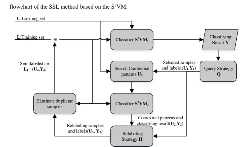
In order to expand L, the semilabeled samples are selected from U iteratively. Fig. 3 shows the 21

flowchart of the SSL method based on the S3_VM. 22

Classifier S3_VM 1

Eliminate duplicate samples L:Training set

Semilabeled set

L1= (U4,Y4) Query Strategy

Q Search Contextual

patterns U2

Classifier S3_VM 2

Selected samples and labels (U1,Y1)

Relabeling samples and labels(U3, Y3)

U:Learning set

⊕

Relabeling Strategy H

Classifying Result Y

Contextual patterns and classifying result(U2,Y2)

23

First, L is processed by the S3_VM

1,during which the label Y of the U is obtained. The subset (U1, Y1) is

1

selected by the query function Q. Then, the context patterns U2of the U1 is found from the U and

2

classified by the S3_VM

2.U2along with the central pattern (U1,Y1) are relabeled by H to get the

3

semilabeled set (U3,Y3). Last, the repeated samples between Land (U3,Y3) are eliminated to obtain the

4

ultimate semilabeled set L1= (U4, Y4)to be added into L. The entire process is iterated until the

5

predefined convergence condition is satisfied, e.g., the total number of the semilabeled samples or the 6

classification accuracy is reached (Pasolli et al. 2014). 7

Next, the implementation of the S3_{VM, the query function Q, the search contextual patterns and} 8

relabeling strategy H are described. 9

2.2S3_{VM method} 10

The S3_{VM is the expansion of the SVM. A standard SVM is based on the structural risk minimization} 11

to classify the learning set by extracting the support vectors from the training set to find the optimal 12

hyper plane(Scholkopf et al. 1997). In case of the binary SVM, given the training set Land the testing 13

set U, it is limited to the following constrained optimization problem (Izquierdo-Verdiguier et al.

14

2013): 15

 

Subject t 1

min ( ) ( )

2

[ 1 1, ,

0 o ] n T i i T i i i C

y b i n

            



w w w

w x

： (3)

16

Where xi is the training sample and yi is the corresponding label,(xi,yi)∈ 𝐋;Φ(∙) maps the data into the 17

feature space; w is the orthogonal vector between xi and the hyper plane; b is the bias to measure 18

the distance between L and the hyper plane; ξi is the slack variable to represent offset of xi; Cis the cost 19

factor to measure the weight between the optimal hyper plane and the minimum offset; n is the number 20

of the training samples. 21

After the initialization, the iterative process is operated and the semilabeled samples (selected from U

22

in the previous step) are added to L. Their confidence is diverse in different iterative steps and they are 23

given different cost factors(Bovolo et al. 2008), which leads to the following cost function for the 24

classifier learning : 25

 

 

1 1

1

min ( ) ( )

2

[ ] 1

ˆ [ ˆ ]

Subject t 1 0 1, , 1, , o , 0 n m T

i j j

i j

T

i i i

T

j j j

i j

C C

y x i n

j n

b

y x b

                          

 

w w w

w

w

： ₍₄₎

26

where𝑥̂𝑗is the semilabled sample selected from U, with the slack variable(εj),cost factor (Cj) and 27

semilabel(𝑦̂𝑗), and nis the number of the semilabeled samples.

28

Applying the Lagrange Duality, the equation (4) can be transformed into the dual problem, which can 29

, 1 1 , 1 , 1 1 1

1 1

1 1

ˆ ˆ ˆ

Subject t

ˆ ˆ ˆ

( , ) ( , ) ( , )

2 2

ˆ 0

0 1, ,

:

0 o

max

i

n m n m n m

i j i j i j i j i j i j i j i j i j i j

i j i j i j i j

n m

i j j

i j

i

j

y y K x x y y K x x y y K x x

y y

C i n

                                     















C j m

 

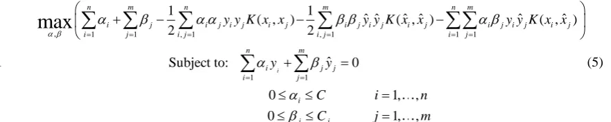
(5) 1

where K=(xi,𝑥̂𝑗𝑗)is a kernel function to calculates the inner product<Φ(xi)∙Φ(𝑥̂𝑗)>;αi and βj are the 2

Lagrange multipliers corresponding to the labeled sample (xi) and the semilabeled sample (𝑥̂𝑗)

3

respectively. When αi and βj are solved by(5), b is solved by 4 1 1 ˆ ˆ ( ) ( ) ( , ) ( , ) n m T

i i i j j j

i j

f x





 

 

   _  _







w (6)

5

Finally, the unlabeled sample x(x∈U) can be labeled by the following decision function: 6

1 1

ˆ ˆ

sgn{( ) } sgn ( , ) ( , )

n m

T

i i i j j j

i j

y x b a y K x x  y K x x b

                     





w (7)

7

It is worth noting that with the increase of iteration, the previous semilabeled samples are more 8

convincing and the corresponding Cj would get bigger. The S3VM can deal with the nonlinear problem 9

using many different kernel functions, such as Gauss kernel function, radial kernel function or 10

exponential kernel function. 11

The basic structure of the S3_{VM is described above. The learning set U and the result Y classified by} 12

the S3_VM

1 are the inputs to Q that is described next. 13

2.3Query Strategy Q 14

Fig. 2 shows the structure of the query strategy Q consisting of two parts Q1 and Q2. Q1is used to screen 15

(U, Y) from (U, Y).Then, (U, Y) is refined by Q2using the proposed rules f1 and f2, and the output 16

is(U1, Y1).

17

Query Strategy Q2 Query Method：f1 Query

Strategy Q1 Learning set and

labels (U,Y)

Query Method：f2

Selected samples and labels (U1,Y1)

Temporary result (U',Y')

18

Fig. 2Structure of Q 19

2.3.1 The implementation of Q1 and Q2 20

Q1is designed on the basis of the MS. The MS is conducive to the convergence of the algorithm 21

because the samples within the margin band are more informative than others. Therefore, Uis selected 22

within the margin band, where the absolute value of the decision function is limited between the ρ and 23





Subject to ( )

i i i

T

i i i

x x abs value i m

value f x x b



     

  

U U

w

： (8)

1

Q2is designed by using the Euclidean distance between the samples and the screening samples from the 2

Uby applying the rules f1and f2.The implementation is shown as follows: 3

I. The distance (D) between the sample of Uand the training set L is calculated by 4

{d_ij|d_ij norm( ,x x_{i j}),x_i ,x_j }

   

D U' L (9)

5

II. The minimum, maximum and their ratios between Uand L are calculated by 6





min d di| i min (j dij),dij

D D (10)

7





max d di| i max (j dij),dij

D D (11)

8





  min

max

D D

 (12)

9

III. The rulef1 is used to select x1 from U: 10

1 1

Subjected to

: ( )

( ) max( ), 1,..., :

f x i

i i k

 

 

max max

U

D D (13)

11

IV. The rulef2 is used toselectx2fromU: 12

2 2

Subjected to

: ( )

( ) max( )

: , 1,...,

f x i

i i k

 

 

U

  (14)

13

V. Finally, update U1:

14

1 2

=  x x

1 1

U U (15)

15

Through the loop running I-V, U1 is updated continuously until the number of samples in U1 reaches

16

the threshold. 17

The implementation of Q has been introduced. Next, the significance off1 and f2is described to prove 18

the rationality of Q. 19

2.3.2 Significance of f1 andf2 20

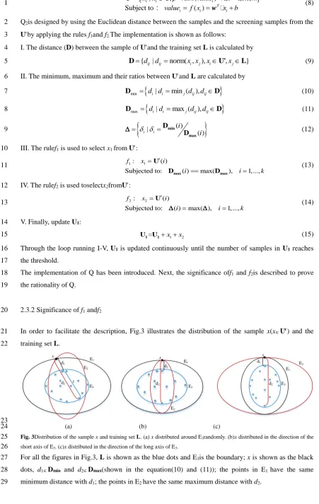
In order to facilitate the description, Fig.3 illustrates the distribution of the sample x(xU) and the 21

training set L. 22 d2 d1 E1 E3 E2 x d2 d1 E1 E3 E2 x d2 d1 E1 E3 E2 x t 23

(a) (b) (c)

24

Fig. 3Distribution of the sample x and training set L. (a) x distributed around E3randomly. (b)x distributed in the direction of the 25

short axis of E3. (c)x distributed in the direction of the long axis of E3. 26

For all the figures in Fig.3, L is shown as the blue dots and E3is the boundary; x is shown as the black 27

dots, d1Dmin and d2Dmax(shown in the equation(10) and (11)); the points in E1 have the same 28

For thef1, Fig. 3(a) shows that the bigger d2generates a longer distance between x and L, and a smaller 1

probability of x belonging to L, so more information is contained in xwhich can decrease the amount 2

of the semilabeled samples used by the SSL. Therefore, f1canselectthe informative sample and reduce 3

the semilabeled samples to the greatest extent. 4

For the f2,Fig. 3(a) shows that the δ (δ∈Δ,in (12))in x can be written as 5

δ= d1/d2 (16)

6

In order to facilitate the description of f2, the expression of δ needs to be changed. 7

Let: d1= d2-t (17)

8

Where t is the secant of x in E3, then substitute (17) into (16): 9

δ = (d2-t)/d2 (18)

10

Get: δ = 1-t/d2 (19)

11

where it can be seen that: when d2 is invariant, the bigger δ is, the smaller t is, which means that x 12

would be closer to the short axis of E3(shown in Fig. 3(b)) and can make distribution of L more 13

uniform (compared with Fig. 3(c));when t is constant, the bigger δ is, the smallerd2is, and the longer 14

distance between x and Lis, which means that the smaller of the probability of x belonging to the L, so 15

the more information that x contains. Therefore, f2cannot only reduce the semilabeled samples by 16

selecting informative ones, but also make the distribution of L better. 17

2.4Search contextual patterns 18

This function makes the current pixel x(x∈U1) as the center sample to find the context patterns U2 from

19

the neighborhood. There are many choices forU2. Espinola et al. (2015)introduced the most

20

common types shown in Fig.4, where Von Neumann neighborhood and Moore neighborhood are called 21

the first-order system and the second-order system(Bruzzone and Persello 2009), and Von Neumann 22

neighborhood is also called the four-directly neighbored pixels (Zhao et al. 2013). 23

24

(a) (b) (c)

25

Fig. 4 Examples of neighborhood systems. (a) Von Neumann neighborhood, (b) Moore neighborhood and (c) Extended Moore 26

neighborhood 27

Context information is very significant. Firstly, the center sample and the context patterns are close in 28

the space, which makes their characteristics exist great relevance that can be applied to calculate the 29

image texture feature(D'Elia et al. 2014)or generate the classification map(Bruzzone and Persello 2009). 30

More semilabeled samples are found using context information, which can improve the convergence 31

speed for the SSL. Secondly, their labels can also provide very important information. In(Espinola et al.

32

2015), the cell automaton distinguishes the different pixels (such as the boundary, noise, or common) at 33

properly using the context information of labels. The next section describes the way to relabel samples 1

by using the information of labels. 2

2.5 H: Relabeling samples 3

Q selects the samples between the maximum margin bands, where the selected samples are more likely 4

to be contaminated and mislabeled manually. To increase the reliability of the selected samples, the 5

central samples (U1,Y1) and the context patterns (U2,Y2)are relabeled by the function H with the

6

following rules: 7

I. When Y2are consistent with Y1, they are left;

8

II. When Y2are inconsistent with Y1, Y1 is incorrect. To make L representative, the corresponding

9

central sample is discarded and the context patterns are left. 10

III. When a part of Y2 is consistent withY1, forY2, the inconsistent context patterns are removed; for Y1,

11

the proportion of consistent part to context patterns is calculated: if the proportion is greater than 12

the threshold, rules A would be followed, else rules B would be chosen. 13

The semilabeled set (U3,Y3) is obtained after being relabeled by H. Then, those samples repeated with

14

L are eliminated, which generates the semilabeled set L1= (U4,Y4)to add to L.

15

Section 2.1-2.5 describes the proposed SSL based method. In order to overcome the influence of the 16

randomness of the learning set L, the classification results are fused in the next section. 17

2.6Fusion method 18

Data fusion is a very popular data processing technology to make up for the defects caused by the 19

missing data or noise pollution. It can be used in many methods. The principal component analysis 20

(PCA) extracts the principal components to fuse the training set, and the spectral information and 21

spatial information are combined together to fuse images. Our fusion method is shown in Fig.5,where 22

the part in the dashed rectangular box is the SSL based method proposed in Section 2.1: 23

Select learning set L' by manual DATA

Proposed Method Select learning

set L by manual

Proposed Method

Fusion Classifying result Y

Classifying result Y' 24

Fig. 5Fusion method 25

Firstly, because only a few labeled samples are needed to initialize the training set, the initial L (L' and 26

etc.) are selected from the DATA manually and would not cost a lot. Then, L is processed by the 27

proposed method to classify the learning set U for obtaining the classification result Y. The other initial 28

sets are processed by the same way. Finally, the different classification results (Y,Yand etc.) are treated 29

3 Experiments

1

In this section, the related experiments are designed to measure the performance of the proposed 2

algorithm (Method Proposed, PM) in three aspects. Firstly, to compare PM with the supervised 3

algorithm, the experiments on PM and SVM are carried out. Secondly, to compare PM with the 4

semisupervised algorithm, the experiments on PM, CS4_{VM and PS}3_{VM-D are carried out. Finally, to} 5

further improve the performance of PM, the different experimental results are fused. 6

3.1 Dataset description and parameters setting 7

3.1.1 Dataset Description 8

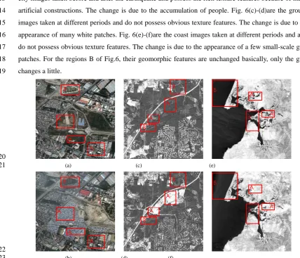
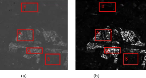
Our experiments on change detection are performed on real RSIs, as shown in Fig. 6, where the regions 9

A and regions B indicate the changed regions and unchanged regions respectively. The aim of change 10

detection is to distinguish the changed part and unchanged part of images (Habib et al. 2009; Celik

11

2010), and can be regarded as the binary classification problem. For the regions A: Fig. 6(a)-(b) are the 12

city images taken before and after the earthquake and possess the rich texture features because of many 13

artificial constructions. The change is due to the accumulation of people. Fig. 6(c)-(d)are the ground 14

images taken at different periods and do not possess obvious texture features. The change is due to the 15

appearance of many white patches. Fig. 6(e)-(f)are the coast images taken at different periods and also 16

do not possess obvious texture features. The change is due to the appearance of a few small-scale gray 17

patches. For the regions B of Fig.6, their geomorphic features are unchanged basically, only the gray 18

changes a little. 19

20

(a) (c) (e)

21

22

(b) (d) (f)

23

Fig. 6 Remote sensing images ofthe city (a) before earthquake and (b) after earthquake, the ground (c) before change and (d) 24

after change, and the coast (a) before change and (b) after change. A represents the changed areas, B represents the unchanged 25

After all the images are processed by the geometric registration and radiometric calibration, then the 1

ratio map of grayscales is generated. To characterize the images, for Fig. 6(a)-(b) the gray level 2

co-occurrence matrix is calculated as the DATA1; for Fig. 6(c)-(d) and Fig. 6(e)-(f), the sample texture

3

featuresare calculated as the DATA2 and DATA3 respectively. All the experimental data are normalized

4

and divided into the training set and the learning set respectively. 5

3.1.2Parameters setting 6

The cost factor C of the PM is nonlinear, defined as follows: 7

2 1

• ( -1)

C N C (20)

8

Where N is the number of iterations; C1 is the initial cost factor; αis the weight coefficient. α and C1are 9

set to 1, and the change range of C is [1,100]. With the increase of iterations, the reliability of the 10

selected samples would increase, and the corresponding C would become larger than the previous one. 11

For the PS3_{VM-D, C is shown in (20), whereC}

1 is set to 2 andαis calculated by 12

2 max min

(C -C ) / (r 1)

  (21)

13

Where Cmax and Cmin are the maximum and minimum of C; r is designed artificially, with r = 10 herein. 14

For the CS4_{VM, C is defined as:} 15

1

2 ( 1)

C  N C (22)

16

where N is also the number of iterations; The initial value of C1 is 2. C is weighted by the K 17

K=C/C=2 (23)

18

When the label of the contextual pattern is the same as the center sample, C is exploited, otherwise C

19

is explored. 20

All the methods are performed using the Gauss kernel function, with the radial width set 0.6. The Von 21

Neumann neighborhood is applied by the PM and CS4_VM. 22

3.2 Comparison with SVM 23

Considering the DATA1, the performance of the SVM and PM is compared. Fig. 7 shows the detection

24

grayscales of the two algorithms. 25

26

(a) (b) 27

Fig. 7 Detection grayscales achieved on DATA1in terms of (a) SVM and (b) PM.A represents the changed areas, B represents the

28

unchanged areas 29

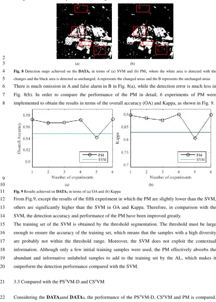
Through the threshold processing, the detection maps are obtained, as shown in Fig. 8 where the 30

changed areas and the B represents the unchanged areas. 1

2

(a) (b) 3

Fig. 8 Detection maps achieved on the DATA1 in terms of (a) SVM and (b) PM, where the white area is detected with the

4

changes and the black area is detected as unchanged; A represents the changed areas and the B represents the unchanged areas 5

There is much omission in A and false alarm in B in Fig. 8(a), while the detection error is much less in 6

Fig. 8(b). In order to compare the performance of the PM in detail, 6 experiments of PM were 7

implemented to obtain the results in terms of the overall accuracy (OA) and Kappa, as shown in Fig. 9. 8

9

(a) (b)

10

Fig. 9 Results achieved on DATA1 in terms of (a) OA and (b) Kappa

11

From Fig.9, except the results of the fifth experiment in which the PM are slightly lower than the SVM, 12

others are significantly higher than the SVM in OA and Kappa. Therefore, in comparison with the 13

SVM, the detection accuracy and performance of the PM have been improved greatly. 14

The training set of the SVM is obtained by the threshold segmentation. The threshold must be large 15

enough to ensure the accuracy of the training set, which means that the samples with a high diversity 16

are probably not within the threshold range. Moreover, the SVM does not exploit the contextual 17

information. Although only a few initial training samples were used, the PM effectively absorbs the 18

abundant and informative unlabeled samples to add to the training set by the AL, which makes it 19

outperform the detection performance compared with the SVM. 20

3.3 Compared with the PS3_{VM-D and CS}4_VM 21

Considering the DATA2and DATA3, the performance of the PS3VM-D, CS4VM and PM is compared.

22

1

(a) (b) (c)

2

Fig. 10 Detection grayscales achieved on DATA2 in terms of (a) CS4VM, (b) PS3VM-D and (c) PM.A represents the changed

3

areas, B represents the unchanged areas 4

5

(a) (b) (c)

6

Fig. 11 Detection grayscales achieved on DATA3 in terms of (a) CS4VM, (b) PS3VM-D and (c) PM.A represents the changed

7

areas, B represents the unchanged areas 8

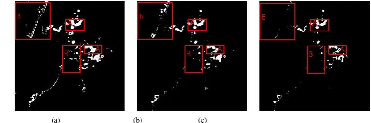
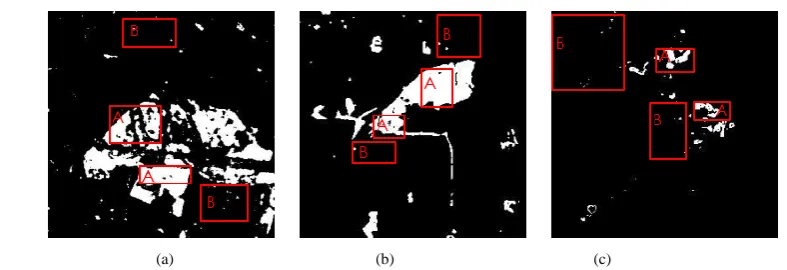
Through the threshold processing, the detection maps of DATA2 and DATA3are obtained, as shown in

9

Fig. 12 and Fig. 13 respectively, where the white area is detected with the changes and the black area is 10

detected as unchanged; A represents the changed areas and B represents the unchanged areas. 11

12

(a) (b) (c)

13

Fig. 12 Detection maps achieved on DATA2 in terms of (a) CS4VM, (b) PS3VM-D and (c) PM, where the white area is detected

14

with the changes and the black area is detected as unchanged; A represents the changed areas and the B represents the unchanged 15

areas 16

17

(a) (b) (c)

18

Fig. 13 Detection maps achieved on DATA3 in terms of (a) CS4VM, (b) PS3VM-D and (c) PM, where the white area is detected

with the changes and the black area is detected as unchanged; A represents the changed areas and the B represents the unchanged 1

areas 2

In Fig. 12, the omission of PS3_{VM-D is the least and that of the PM is the greatest in A; the false alarm} 3

of PM is the least and that of the CS4_{VMisthegreatest in B. It can be seen that the performance of the} 4

three algorithms is ideal and that of PM is more accurate than others for DATA2. In Fig.13, the false

5

alarm of PM is significantly less than that of the other algorithms in B, followed by thePS3_{VM-D. The} 6

omission of three algorithms is almost the same in A. Therefore, the detection result of PM is the best 7

for DATA3.

8

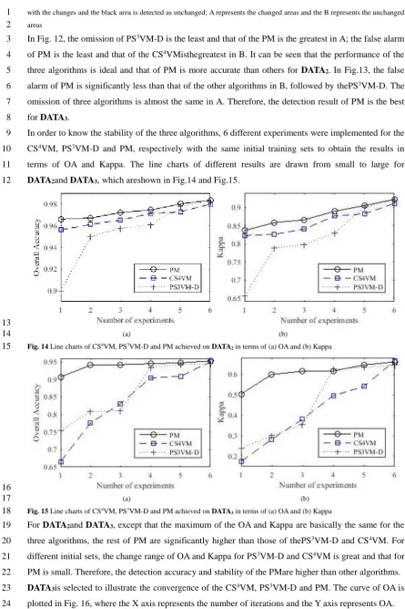
In order to know the stability of the three algorithms, 6 different experiments were implemented for the 9

CS4_{VM, PS}3_{VM-D and PM, respectively with the same initial training sets to obtain the results in} 10

terms of OA and Kappa. The line charts of different results are drawn from small to large for 11

DATA2and DATA3, which areshown in Fig.14 and Fig.15.

12

13

(a) (b)

14

Fig. 14 Line charts of CS4_{VM, PS}3_{VM-D and PM achieved on DATA}

2 in terms of (a) OA and (b) Kappa

15

16

(a) (b) 17

Fig. 15 Line charts of CS4_{VM, PS}3_{VM-D and PM achieved on DATA}

3 in terms of (a) OA and (b) Kappa

18

For DATA2and DATA3, except that the maximum of the OA and Kappa are basically the same for the

19

three algorithms, the rest of PM are significantly higher than those of thePS3_{VM-D and CS}4_{VM. For} 20

different initial sets, the change range of OA and Kappa for PS3_{VM-D and CS}4_{VM is great and that for} 21

PM is small. Therefore, the detection accuracy and stability of the PMare higher than other algorithms. 22

DATA3is selected to illustrate the convergence of the CS4VM, PS3VM-D and PM. The curve of OA is

23

1

Fig. 16 Line charts of PM achieved on DATA3

2

With the increase of iterations, the OAs of the three algorithms all change, where the OA of the CS4_VM 3

increases from 0.64 to 0.79, the OA of thePS3_{VM-D increases from 0.64 to 0.82 and the OA of PM} 4

increases from 0.64 to 0.94. The curve of the PM rises fastest, which suggests that the PM can get the 5

faster convergence speed than other algorithms. 6

The CS4_{VM can increase the relevance of the training samples by searching the contextual samples,} 7

but it does not consider whether those samples are beneficial to improve the convergence rate. The 8

PS3_{VM-D guarantees the information of the selected samples by searching them within the margin} 9

band, but the probability that these samples are polluted is also great. Compared to the CS4_{VM and the} 10

PS3_{VM-D, the PM uses the AL to select the informative samples, then use the context information to} 11

increase the samples correlation, which improves the detection accuracy and ensures the reliability of 12

the selected samples. We use a new query function Q to make the distribution of the training samples 13

more uniform for improving the detection efficiency and accuracy. Moreover, the convergence of the 14

PM is further improved by applying the semilabeled samples. 15

3.4Fusion for PM 16

To obtain the more accurate results and verify the effectiveness of the fusion for the SSL methods, the 17

experimental results of the PM are fused. The OA and Kappa are listed in Table 1, and the fusion 18

detection maps are shown in Fig. 17, where the white area is detected with the changes and the black 19

area is detected as unchanged. A represents the changed areas and B represents the unchanged areas. 20

21

(a) (b) (c)

22

Fig. 17 Fusion detection maps achieved on (a) DATA1, (b) DATA2and (c) DATA3for PM, where the white area is detected with

23

the changes and the black area is detected as unchanged; A represents the changed areas and the B represents the unchanged areas 24

Table 1OA and Kappa of different experiments for DATA1, DATA2 and DATA3

1 2 3 4 5 6 Fusion OA Kappa OA Kappa OA Kappa OA Kappa OA Kappa OA Kappa OA Kappa DATA1 0.9718 0.8955 0.9662 0.8839 0.9668 0.8760 0.9717 0.8997 0.9413 0.8045 0.9724 0.8977 0.9744 0.9060 DATA2 0.9659 0.8582 0.9721 0.8661 0.9835 0.9225 0.9800 0.9053 0.9670 0.8365 0.9744 0.8894 0.9837 0.9250 DATA3 0.9475 0.6155 0.9420 0.6139 0.9409 0.6447 0.9451 0.5991 0.9072 0.5031 0.9528 0.6599 0.9534 0.6638

In TABEL 1, both the OA and Kappa get higher after fusion. By comparing Fig. 17(a), Fig. 17(b) and 1

Fig. 17(c) with Fig. 8(b), Fig. 12(c) and Fig. 13(c) respectively, it is found that the false alarm in B and 2

the omission in A reduces a lot after the fusion for DATA1 and DATA3. The false alarm in B region and

3

the omission in A decreases slightly for DATA2. Obviously, the data fusion could effectively

4

compensate the detection error, reduce the risk caused by the different initial training sets and improve 5

the detection accuracy. 6

4. Conclusion

7

In this paper, a novel method is proposed for the change detection of RS images. It fully incorporates 8

the methods and concepts in the SSL, and adopts them to fit the situation where the labeled samples are 9

insufficient. 10

The novelty of this paper lies in: a) By considering the advantages of the AL and the context 11

information, a novel semisupervised method is designed; b) by analyzing the distribution of the 12

samples, a new query function is designed to select the semilabeled samples using the Euclidean 13

distance; c) Based on the idea of data fusion, the discrete results of the PM are effectively fused. In the 14

experiments of change detection for actual RSIs, the PM has made a significant improvement in the 15

detection accuracy, convergence rate, and the stability in comparison with other existing methods. It 16

can be further improved by using other effective fusion methods. 17

References

18

Anand, S., Mittal, S., Tuzel, O., & Meer, P. (2014). Semi-Supervised Kernel Mean Shift Clustering. Pattern Analysis and

19

Machine Intelligence, IEEE Transactions on, 36(6), 1201-1215, doi:10.1109/TPAMI.2013.190. 20

Bazi, Y., Melgani, F., & Al-Sharari, H. D. (2010). Unsupervised change detection in multispectral remotely sensed imagery with 21

level set methods. Geoscience and Remote Sensing, IEEE Transactions on, 48(8), 3178-3187. 22

Bovolo, F., Bruzzone, L., & Marconcini, M. (2008). A Novel Approach to Unsupervised Change Detection Based on a 23

Semisupervised SVM and a Similarity Measure. Geoscience and Remote Sensing, IEEE Transactions on, 46(7), 24

2070-2082, doi:10.1109/TGRS.2008.916643. 25

Bruzzone, L., & Persello, C. (2009). A Novel Context-Sensitive Semisupervised SVM Classifier Robust to Mislabeled Training 26

Samples. Geoscience and Remote Sensing, IEEE Transactions on, 47(7), 2142-2154, 27

doi:10.1109/TGRS.2008.2011983. 28

Celik, T. (2010). Change Detection in Satellite Images Using a Genetic Algorithm Approach. Geoscience and Remote Sensing

29

Letters, IEEE, 7(2), 386-390, doi:10.1109/LGRS.2009.2037024. 30

Chapelle, O., Schölkopf, B., & Zien, A. (2006). Semi-supervised learning. 31

D'Elia, C., Ruscino, S., Abbate, M., Aiazzi, B., Baronti, S., & Alparone, L. (2014). SAR Image Classification Through 32

Information-Theoretic Textural Features, MRF Segmentation, and Object-Oriented Learning Vector Quantization. 33

Selected Topics in Applied Earth Observations and Remote Sensing, IEEE Journal of, 7(4), 1116-1126, 34

doi:10.1109/JSTARS.2014.2304700. 35

Demir, B., Persello, C., & Bruzzone, L. (2011). Batch-Mode Active-Learning Methods for the Interactive Classification of 36

Remote Sensing Images. Geoscience and Remote Sensing, IEEE Transactions on, 49(3), 1014-1031, 37

Didaci, L., Fumera, G., & Roli, F. (2012). Analysis of Co-training Algorithm with Very Small Training Sets. In G. Gimel’farb, E. 1

Hancock, A. Imiya, A. Kuijper, M. Kudo, S. Omachi, et al. (Eds.), Structural, Syntactic, and Statistical Pattern

2

Recognition (Vol. 7626, pp. 719-726, Lecture Notes in Computer Science): Springer Berlin Heidelberg. 3

Espinola, M., Piedra-Fernandez, J. A., Ayala, R., Iribarne, L., & Wang, J. Z. (2015). Contextual and Hierarchical Classification of 4

Satellite Images Based on Cellular Automata. Geoscience and Remote Sensing, IEEE Transactions on, 53(2), 795-809, 5

doi:10.1109/TGRS.2014.2328634. 6

Geiß, C., & Taubenböck, H. (2013). Remote sensing contributing to assess earthquake risk: from a literature review towards a 7

roadmap. Natural Hazards, 68(1), 7-48, doi:10.1007/s11069-012-0322-2. 8

Gomez-Chova, L., Bruzzone, L., Camps-Valls, G., & Calpe-Maravilla, J. Semi-Supervised Remote Sensing Image Classification 9

based on Clustering and the Mean Map Kernel. In Geoscience and Remote Sensing Symposium, 2008. IGARSS 2008.

10

IEEE International, 7-11 July 2008 2008 (Vol. 4, pp. IV - 391-IV - 394). doi:10.1109/IGARSS.2008.4779740. 11

Gong, C., Junwei, H., Lei, G., Zhenbao, L., Shuhui, B., & Jinchang, R. (2015). Effective and Efficient Midlevel Visual 12

Elements-Oriented Land-Use Classification Using VHR Remote Sensing Images. Geoscience and Remote Sensing,

13

IEEE Transactions on, 53(8), 4238-4249, doi:10.1109/TGRS.2015.2393857. 14

Habib, T., Inglada, J., Mercier, G., & Chanussot, J. (2009). Support Vector Reduction in SVM Algorithm for Abrupt Change 15

Detection in Remote Sensing. Geoscience and Remote Sensing Letters, IEEE, 6(3), 606-610, 16

doi:10.1109/LGRS.2009.2020306. 17

Hansen, M. C., & Loveland, T. R. (2012). A review of large area monitoring of land cover change using Landsat data. Remote

18

Sensing of Environment, 122, 66-74, doi:http://dx.doi.org/10.1016/j.rse.2011.08.024. 19

Hearst, M. A., Dumais, S. T., Osman, E., Platt, J., & Scholkopf, B. (1998). Support vector machines. Intelligent Systems and their

20

Applications, IEEE, 13(4), 18-28, doi:10.1109/5254.708428. 21

Izquierdo-Verdiguier, E., Laparra, V., Gomez-Chova, L., & Camps-Valls, G. (2013). Encoding Invariances in Remote Sensing 22

Image Classification With SVM. Geoscience and Remote Sensing Letters, IEEE, 10(5), 981-985, 23

doi:10.1109/LGRS.2012.2227297. 24

Junwei, H., Dingwen, Z., Gong, C., Lei, G., & Jinchang, R. (2015a). Object Detection in Optical Remote Sensing Images Based 25

on Weakly Supervised Learning and High-Level Feature Learning. Geoscience and Remote Sensing, IEEE

26

Transactions on, 53(6), 3325-3337, doi:10.1109/TGRS.2014.2374218. 27

Junwei, H., Dingwen, Z., Xintao, H., Lei, G., Jinchang, R., & Feng, W. (2015b). Background Prior-Based Salient Object 28

Detection via Deep Reconstruction Residual. Circuits and Systems for Video Technology, IEEE Transactions on, 25(8), 29

1309-1321, doi:10.1109/TCSVT.2014.2381471. 30

Kawakita, M., & Kanamori, T. (2013). Semi-supervised learning with density-ratio estimation. Machine Learning, 91(2), 31

189-209, doi:10.1007/s10994-013-5329-8. 32

Li, J., Bioucas-Dias, J. M., & Plaza, A. (2010). Semisupervised Hyperspectral Image Segmentation Using Multinomial Logistic 33

Regression With Active Learning. Geoscience and Remote Sensing, IEEE Transactions on, 48(11), 4085-4098, 34

doi:10.1109/TGRS.2010.2060550. 35

Maulik, U., & Chakraborty, D. (2012). A novel semisupervised SVM for pixel classification of remote sensing imagery. 36

International Journal of Machine Learning and Cybernetics, 3(3), 247-258, doi:10.1007/s13042-011-0059-3. 37

Maulik, U., & Chakraborty, D. (2014). Fuzzy Preference Based Feature Selection and Semisupervised SVM for Cancer 38

Classification. NanoBioscience, IEEE Transactions on, 13(2), 152-160, doi:10.1109/TNB.2014.2312132. 39

Munoz-Mari, J., Tuia, D., & Camps-Valls, G. (2012). Semisupervised Classification of Remote Sensing Images With Active 40

Queries. Geoscience and Remote Sensing, IEEE Transactions on, 50(10), 3751-3763, 41

doi:10.1109/TGRS.2012.2185504. 42

Pasolli, E., Melgani, F., Tuia, D., Pacifici, F., & Emery, W. J. (2014). SVM Active Learning Approach for Image Classification 43

Using Spatial Information. Geoscience and Remote Sensing, IEEE Transactions on, 52(4), 2217-2233, 44

doi:10.1109/TGRS.2013.2258676. 45

Persello, C., & Bruzzone, L. (2014). Active and Semisupervised Learning for the Classification of Remote Sensing Images. 46

Geoscience and Remote Sensing, IEEE Transactions on, 52(11), 6937-6956, doi:10.1109/TGRS.2014.2305805. 47

Schohn, G., & Cohn, D. Less is more: Active learning with support vector machines. In ICML, 2000 (pp. 839-846): Citeseer 48

Scholkopf, B., Kah-Kay, S., Burges, C. J. C., Girosi, F., Niyogi, P., Poggio, T., et al. (1997). Comparing support vector machines 49

2758-2765, doi:10.1109/78.650102. 1

Shahshahani, B. M., & Landgrebe, D. A. (1994). The effect of unlabeled samples in reducing the small sample size problem and 2

mitigating the Hughes phenomenon. Geoscience and Remote Sensing, IEEE Transactions on, 32(5), 1087-1095, 3

doi:10.1109/36.312897. 4

Tuia, D., Volpi, M., Copa, L., Kanevski, M., & Munoz-Mari, J. (2011). A Survey of Active Learning Algorithms for Supervised 5

Remote Sensing Image Classification. Selected Topics in Signal Processing, IEEE Journal of, 5(3), 606-617, 6

doi:10.1109/JSTSP.2011.2139193. 7

Yi, Y., Wu, J., & Xu, W. (2011). Incremental SVM based on reserved set for network intrusion detection. Expert Systems with

8

Applications, 38(6), 7698-7707. 9

Zhao, C., Li, X., Ren, J., & Marshall, S. (2013). Improved sparse representation using adaptive spatial support for effective target 10

detection in hyperspectral imagery. International Journal of Remote Sensing, 34(24), 8669-8684, 11

doi:10.1080/01431161.2013.845924. 12

Zhu, X. (2010). Semi-Supervised Learning. In C. Sammut, & G. Webb (Eds.), Encyclopedia of Machine Learning (pp. 892-897): 13

Springer US. 14

Author Biographies

15

FeiGao received the B.S. and M.S. degree from the Xi’an Petroleum Institute, Xi’an, China, in 1996 16

and 1999, respectively, and the Ph.D. degrees from Beijing University of Aeronautics and Astronautics 17

(BUAA), Beijing, China, in 2005. He is currently an Associate Professor with the School of Electronic 18

and Information Engineering, BUAA. He is interested in radar signal processing, moving target 19

detection and image processing. 20

21 22 23

Wenchao Lv received the B.S. degree in electronic and information engineering fromBeijing 24

University of Posts and Telecommunications, Beijing, China, in 2014. He is currently pursuing the 25

M.E. degree in electronic and communication engineering at Beijing University of Aeronautics and 26

Astronautics, Beijing, China. His current research activity is in machine learning and synthetic aperture 27

radar image classification. 28

29 30

31

Yaotian Zhang received the B.S. degree in Electronic Engineering from BeihangUniversityin 2003. He 32

was awarded Ph.D degree in Signal Processing from Beihang University in 2009. Since2010, he has 33

worked in School of Electronic and Information Engineering of Beihang University as an assistant 34

professor. His research interest covers image understanding, target detection and Micro-Doppler signal 35

analysis. 36

37 38 39

Jinping Sun received the M.Sc. and Ph.D. degrees from the Beijing University of Aeronautics and 40

Astronautics (BUAA), Beijing, China, in 1998 and 2001, respectively. He is currently a Professor with 41

the School of Electronic and Information Engineering, BUAA. His research interests include 42

high-resolution radar signal processing, image understanding, and robust beamforming. 43

44 45 46 47

Jun Wang received the B.S. degree from the Northwestern Polytechnical University, Xi’an, China, in 48

(BUAA), Beijing, China, in 1998 and 2001, respectively. He is currently a Professor with the School of Electronic and 1

Information Engineering, BUAA. He is interested in signal processing, DSP/FPGA real-time architecture, target recognition and 2

tracking, and so on. His research has resulted in 38 papers in journals, books, and conference proceedings. 3

4 5

Erfu Yang is a Lecturer in the Department of Design Manufacture and Engineering Management 6

(DMEM) at the University of Strathclyde, Glasgow, UK. His main research interests include robotics, 7

autonomous systems, mechatronics, manufacturing automation, computer vision, image/signal 8

processing, nonlinear control, process modelling and simulation, condition monitoring, fault diagnosis, 9

multi-objective optimizations, and applications of machine learning and artificial intelligence including 10

multi-agent reinforcement learning, fuzzy logic, neural networks, bio-inspired algorithms, and cognitive 11

computation, etc. He has over 60 publications in these areas, including more than 30 journal papers and 12