Estimation of particle size distribution and aspect ratio of non-spherical particles from chord length distribution

Estimation of Particle Size Distribution and Aspect

Ratio of Non-Spherical Particles From Chord Length

Distribution

Okpeafoh S. Agimelena,∗, Peter Hamiltonb, Ian Haleyc, Alison Nordonb, Massimiliano Vasiled_{, Jan Sefcik}a_{, Anthony J. Mulholland}e

a_{Department of Chemical and Process Engineering, University of Strathclyde, James}

Weir Building, 75 Montrose Street, Glasgow, G1 1XJ, United Kingdom.

b_{WestCHEM, Department of Pure and Applied Chemistry and Centre for Process}

Analytics and Control Technology, University of Strathclyde, 295 Cathedral Street, Glasgow, G1 1XL, United Kingdom

c_{Mettler-Toledo Ltd., 64 Boston Road, Beaumont Leys Leicester, LE4 1AW, United}

Kingdom

d_{Department of Mechanical and Aerospace Engineering, University of Strathclyde, James}

Weir Building, 75 Montrose Street, Glasgow, G1 1XJ, United Kingdom.

e_{Department of Mathematics and Statistics, University of Strathclyde, Livingstone}

Tower, 26 Richmond Street, Glasgow G1 1XH, United Kingdom

Abstract

Information about size and shape of particles produced in various manu-facturing processes is very important for process and product development because design of downstream processes as well as final product properties strongly depend on these geometrical particle attributes. However, recovery of particle size and shape information in situ during crystallisation processes has been a major challenge. The focused beam reflectance measurement (FBRM) provides the chord length distribution (CLD) of a population of particles in a suspension flowing close to the sensor window. Recovery of size and shape information from the CLD requires a model relating particle size and shape to its CLD as well as solving the corresponding inverse problem.

This paper presents a comprehensive algorithm which produces estimates of particle size distribution and particle aspect ratio from measured CLD

∗_{Corresponding author}

data. While the algorithm searches for a global best solution to the in-verse problem without requiring further a priori information on the range of particle sizes present in the population or aspect ratio of particles, suitable regularisation techniques based on relevant additional information can be im-plemented as required to obtain physically reasonable size distributions. We used the algorithm to analyse CLD data for samples of needle-like crystalline particles of various lengths using two previously published CLD models for ellipsoids and for thin cylinders to estimate particle size distribution and shape. We found that the thin cylinder model yielded significantly better agreement with experimental data, while estimated particle size distribu-tions and aspect ratios were in good agreement with those obtained from imaging.

Keywords: Chord Length Distribution, Particle Size Distribution, Particle Shape, Focused Beam Reflectance Measurement.

1. Introduction

sen-sitive to particle shape, extracting accurate shape information has been chal-lenging since appropriate models need to be used and corresponding inverse problems need to be solved. Suspensions also need to be relatively dilute for laser diffraction measurements in order to avoid multiple scattering effects.

Reflectance techniques, such as FBRM, are particularly suitable for in situ monitoring of particles in suspensions during the manufacturing pro-cess. FBRM measures chord length distribution (CLD), which depends on both size and shape of particles present in a suspension. There has been con-siderable efforts [3–15] devoted towards obtaining useful information about particle geometrical attributes from this technique, leading to the develop-ment of suitable models [3–9,11–15] for CLDs for particles of various shapes in order to obtain particle size distributions from FBRM data.

However, the inverse problem of retrieving size and shape information from FBRM data is non-trivial [2]. The inverse problem is well-known to be ill-posed, i.e., there are potentially multiple solutions in terms of particle size distributions and shape which give essentially the same CLD within the accuracy of experimental data. Several regularisation approaches have been proposed to deal with this problem [8, 9] but there is still a challenge of finding a global best solutions for physically reasonable combinations of particle size distribution and shape. One important factor which can be used to constrain inverse problem solutions is the size range of particles used in the calculations. In the work by Ruf et al [4] information about particle size range was obtained by a laser diffraction technique and microscopy, while Worlitschek et al. [8], Li et al. [10], Li et al. [16, 17] and Yu et al. [18] obtained particle size range information by sieving. Also, Kail et al. [14] obtained information about particle size range in their population of particles from the manufacturer. However, information about particle size range may not be readily available or it may not be convenient to obtain this information a priori (for example in a manufacturing process).

When moving from modelling of CLD of single particles to a population of particles of various sizes, it is necessary to properly account for size effects. It has been previously shown [11,19,20] (see also section 3 of the supplementary information) that probability of larger particles to be detected by the FBRM probe is proportional to their characteristic size. While this effect has been taken into account in some cases [4, 8] it has been neglected in some other cases [9,10] in the previous literature, which may introduce significant errors if the size range of particles in the population is relatively large.

spherical particles 1_{. While these models can give reasonable estimates of}

particle sizes from measured CLD data, if appropriate approaches are used for solving corresponding inverse problems, they are not suitable for parti-cles whose shape deviate significantly from spherical. Even though there has been some progress in retrieving size and shape information from CLD data for populations of particles with different degrees of variation from spherical [4,8–10, 24,25], there has been no previous attempt (although Czapla et al. [26] calculated the CLD of needle shaped particles using a numerical model, the inverse problem was not solved) to obtain size and shape information for populations of needle shaped particles which are commonly present in pharmaceutical manufacturing. This is despite the fact that there are suit-able geometrical models [9,11] available in the literature which can be used to obtain useful size and shape information for needle shaped particles from experimental CLD data.

In this paper, we present an algorithm for estimating of size and shape information for needle shaped particles from experimental CLD data. We use 2 D geometrical CLD models available in the literature which are suitable for opaque particles. However, the method presented here can be extended to different 2 D and 3 D geometrical and optical CLD models for parti-cles of arbitrary shape and optical properties. Such models would need to account for possible discontinuities along the particles’ boundaries if the par-ticles’ boundaries contain strong concavities (for example the case of particle clusters). More general models would also need to account for the optical properties of the particles if the particles are not opaque.

The optimum size range of particles in a population providing the best fit with the experimental CLD data can be directly determined by the algorithm in the case when no further information is available, although any external information on particle size range or shape can be utilised in the algorithm as needed. We compare results from our calculations with data obtained by dynamic image analysis and laser diffraction in order to assess suitability and validity of models used.

1_{The problem is significantly simplified for spherical particles due to the symmetry}

Figure 1: Microscope images (magnification factor of ×150) of samples of COA after undergoing different drying conditions in the vacuum agitated drier [27]. The samples in (a) to (e) are labelled Sample 1 to Sample 5 in Figs. 2 and3. The white horizontal line on the bottom right of (a) indicates a length of 100µm. Reproduced by permission of The Royal Society of Chemistry (View Online).

100 101 102 103

0 100 200 300 400 500 600

Chord Length(µm)

C

o

u

n

ts

Sample# 1 2 3 4 5

100 101 102 103

0 0.5 1 1.5 2 2.5

Particle Diameter(µm)

V

o

l

.

D

e

n

s

it

y

(

µ

m

)

−

1

Sample# 1

2

3

4

5

(b) (a)

Figure 2: (a) Volume based particle size distribution obtained with the Malver Mastersizer and (b) unweighted number based chord length distribution from the FBRM probe for the samples in Fig. 1.

2. Experimental Data

101 102 103 0 5 10 15 20

EQPC(µm)

V o l . D e n s it y ( µ m ) − 1 Sample# 1 2 3 4 5

101 102 103

0 1 2 3 4 5 6

Feret Max(µm)

V o l . D e n s it y ( µ m ) − 1 Sample# 1 2 3 4 5

101 102 103

0 10 20 30 40 50

Feret Min(µm)

V o l . D e n s it y ( µ m ) − 1 Sample# 1 2 3 4 5

1 2 3 4 5

0 0.1 0.2 0.3 0.4 Samples FM in / FM a x (c) (a) (b) (d)

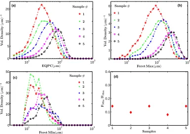
Figure 3: (a) Volume based EQPC diameter, maximum Feret diameter (b), and minimum Feret diameter (c) obtained by dynamic image analysis for the samples in Fig. 1. (d) A measure of the degree of elongation (aspect ratio) of the needles in Fig. 1.

LIXELL wet dispersion unit. Further experimental details for the particle size analysis techniques employed can be found in the previous study [27].

The particle size distribution (volume weighted) estimated by laser diffrac-tion, which assumes that the particles are spherical, for samples 1 to 5 is shown in Fig. 2(a). The CLD data obtained by FBRM for the five samples is shown in Fig. 2(b). The equivalent projected circle EQPC diameter (which is the diameter of a circle of equal area to the 2 D projection of a particle) distribution obtained by dynamic image analysis is shown in Fig. 3(a). The maximum Feret diameter (Feret Max)2 _{obtained using dynamic image}

anal-ysis, which was shown to be a good indicator of needle length [27], is shown in Fig. 3(b). In addition, the Feret Min diameter (Feret Min) which is an

2_{See section 7 of the supplementary information and [27]for further description of the}

indication of needle width is shown in Fig. 3(c). The degree of elongation (aspect ratio) of the needles can be estimated by computing the ratio of the modes of the Feret Min distributions to the modes of the Feret Max distri-butions. The result (Fmin/Fmax) of this calculation is shown in Fig. 3(d).

The data in Figs. 2 and 3 will be used to compare against estimated PSDs and aspect ratios obtained from CLDs data in Fig. 2(b) using the algorithm described in section 4.

3. Modelling Chord Length Distribution

The FBRM technology involves a laser beam which is focused onto a spot by a system of lenses. The focus spot is located near a sapphire window and it is rotated along a circular path at a speed of about 2ms−1 _{[2, 7, 12, 13].}

The assembly of lenses is enclosed in a tubular probe which is inserted into a slurry of dispersed particles. Particles passing near the probe window reflect light back into the probe which is then detected. It is assumed that the particles are much smaller than the diameter of the circular trajectory of the laser beam, and the particles move much more slowly than the speed of the laser spot [2]. Hence the length of arc (taken to be a straight line) made by the laser spot on a particle from which light is back scattered is just a product of the speed of the laser spot and the duration of reflection [2], and the corresponding chord length is recorded. Since the beam does not always pass through the centre of the particle, a range of chord lengths is recorded as a given particle encounters the beam multiple times. The FBRM device accumulates chord lengths across different particles present in the slurry for a duration pre-set by the user, after which it reports a chord length histogram, and this data is referred to as chord length distribution (CLD).

3.1. Calculating CLD from PSD

this function depends on the shape of the particle [11]. For example, in the case of a population of spherical particles of different sizes the characteristic size is D = 2as, where as is the radius of a sphere. Thus the relationship

between the CLD and PSD can be written as [20]

C(L) =

Z ∞

0

A(D, L)DX(D)dD, (1)

where C is the CLD of the particle population, L is chord length and X is the PSD expressed as a normalised number distribution. Equation (1) can be discretised and written in matrix form as [9, 20]

C=A ˜X, (2)

whereAis a transformation matrix. The column vectorCis the chord length histogram or CLD, while the column vector X˜ is defined as

˜

Xi =DiXi, i= 1,2,3, . . . , N, (3)

where D is the vector of characteristic sizes and X is the unknown PSD. The characteristic sizes Di make up the bin boundaries of the PSDXi, and

the characteristic size of the particles bounded by the bin boundariesDi and Di+1 is given asDi =

√

DiDi+1. Equation (2) can be rearranged so that each

component of D multiplies a column of A to give

C=AX˜ , (4)

where

˜

Aj = [aj,1D1 aj,2D2 . . . aj,iDi . . . aj,NDN], (5)

represents column j of A˜.

The matrixA is of dimension M ×N, where M is the number of chord length bins in the histogram Cand N is the number of particle size bins in the histogram X [9]. The columns of matrix A are constructed as [9]

Aj = [aj,1 aj,2 . . . aj,i . . . aj,N], (6)

where

aj,i=pDi(Lj, Lj+1) (7)

for different particle sizes and chord length bins are calculated from appro-priate probability density functions (PDF). The PDFs employed in this work are those given by the Vaccaro-Sefcik-Morbidelli (VSM) [11] model and the Li-Wilkinson (LW) model [9].

The forward problem of calculating the CLD from a known PSD using Eq. (4) is trivial as it is mere matrix multiplication. However, the inverse problem of calculating the PSD from a known CLD is non trivial. The solution vector

X must meet the requirement of non negativity, hence different techniques have been used in the past [8, 9] to fulfil this requirement. There could also be errors in the solution vector X if the transformation matrix A is inaccurate. The accuracy of the matrix Adepends on the particle size range and the model used in calculating the probabilities in Eq. (7). Here we shall describe a technique to select the most appropriate particle size range. The method employed here also guarantees the non negativity requirement of the solution vectorX. Appropriate models then need to be chosen based on any available information about the overall particle shape. In the case of needle-like particles considered here, we can use two analytical models available in the literature as discussed below.

3.2. The VSM model

The microscope images in Fig. 1 suggest that the shape of the particles could be represented by thin cylinders. The 2 D projections of these thin cylinders will look like the shapes in Fig. 1. The cylindrical VSM model [11] gives a PDFXc

p which defines the relative likelihood that a chord taken

from a cylindrical particle has a length between L and L+dL. To this end, the model considers all possible 3 D orientations of each cylindrical particle and calculates chord lengths from each 2 D projection. The characteristic size of a cylinder is calculated by equating to the diameter of a sphere of equivalent volume. For a thin cylinder of height ac, base radius bc, aspect

ratiorc=bc/acand characteristic sizeDc=ac 3 p

3r2

c/2, the VSM model gives

the probability Xc

p (for bc/ac1) as [11]

a∗X_pc(L) =



    

     1 2

L √

r2

ca2c−L2

1−p1−r2 c

, ∀L∈[0, rcac[

1 π

r2

c

q

1−_(acL₎2 +

1 2π

ac

L

L ac

q 1−₍L

ac)

2

+cos−1₍L ac) L

rcac

q

( L rcac)

2

−1 ∀L∈]rcac, ac[

0 ∀L∈[ac,∞[,

where

a∗ = ac 4 +

1 2rcac

1−p1−r2 c +

1 2rc

1− 4 πsin

−1

(rc)

(9)

is a normalisation factor. Then the probability that the length of a measured chord from a particle of size Dc falls in the bin bounded by Lj and Lj+1 is

calculated as

p_cD

i(Lj, Lj+1) =

Z Lj+1

Lj

X_pc(L)dL. (10)

The integration in Eq. (10) is performed numerically.

3.3. The LW model

In this case, we approximate the shape of the needles in Fig. 1 by thin ellipsoids. The model considers 2 D projections of each of ellipsoid with its major and minor axes parallel to the projection plane, so that all projections will be an ellipse of semi major axis length ae, semi minor axis lengthbe and

aspect ratio re=be/ae. The length of a chord on this ellipse depends on the

angle α between the chord and the xaxis (where the projection plane is the

x−y plane) [9]. Hence the PDF for such an ellipse is angular dependent. The PDF for different values of α are given by the LW model as [9]:

for α= 0 or π

p_eD

i(Lj,α, Lj+1,α) =

           r

1− Lj

2aei

2 −

r

1−Lj+1 2aei

2

, forLj < Lj+1 ≤2aei

r

1− Lj

2aei

2

, forLj ≤2aei < Lj+1

0, for 2aei < Lj < Lj+1,

(11) for α=π/2 or 3π/2

p_eD

i(Lj,α, Lj+1,α) =

           r

1− Lj

2reaei

2 −

r

1−Lj+1 2reaei

2

, for Lj < Lj+1 ≤2reaei

r

1− Lj

2reaei

2

, for Lj ≤2reaei < Lj+1

0, for 2reaei < Lj < Lj+1,

for other values of α

p_eD

i(Lj,α, Lj+1,α) =

                     r

1− re2+s2

1+s2

Lj

2reaei

2

− r

1− re2+s2

1+s2

_L

j+1 2reaei

2

, for Lj < Lj+1 ≤2reaei q

1+s2 r2

e+s2

r

1− re2+s2

1+s2

_L

j

2reaei

2

, for Lj ≤2reaei q

1+s2 r2

e+s2 < Lj+1

0, for 2reaei

q 1+s2 r2

e+s2 < Lj < Lj+1,

(13) where s= tan (α). The angle independent PDF is then given as

p_eD

i(Lj, Lj+1) =

1 2π

Z 2π

0 p_eD

i(Lj,α, Lj+1,α)dα. (14)

Equation (14) allows the construction of the transformation matrixAin Eq. (2) which can be converted to the matrix ˜A as described in Eq. (5). The matrix ˜A is then used to solve the inverse problem.

The LW model constructs the PDF of an ellipsoidal particle by consider-ing only one 2 D projection of the ellipsoid where the major axis is parallel to the projection plane. Hence the monotonic function which gives the char-acteristic size De of the resulting ellipse is obtained from the area of a circle

of equivalent area. Hence, using re = be/ae, the characteristic size is given

as De = 2ae √

re.

4. Inversion Algorithm

As mentioned in the introduction, one important factor which can be used to constrain inverse problem solutions is the size range (Dmin toDmax)

of particles used in the calculations, where Dmin is the smallest particle size

andDmaxis the largest particle size in the population. Since this information

is not always readily available, we introduce an inversion algorithm which is capable of automatically determining the best values of Dmin and Dmax to

solve the inverse problem. We use the bin boundaries of the chord length histogram to specify the size range boundaries Dmin andDmax. A numberS

Figure 4: Pictorial representation of the bins and bin boundaries of the CLD histogram showing a window of size S at the first two positions set by p= 1 andp= 2 shifted by q. The window is moved in such a way that some of the bins contained in the window at p= 1 overlap some of the bins of the window atp= 2.

the first two bin boundaries of a window is taken as Dmin and the geometric

mean of the last two bins of a window is taken as Dmax. The procedure is

outlined below.

The boundaries of the chord length histogram are labelled as

Lj, j = 1,2,3, . . . , M + 1 (15)

as illustrated in Fig. 4. The characteristic chord length Lj of bin j is the

geometric mean of the chord lengths of its boundaries

Lj = p

LiLj+1. (16)

At the beginning of the calculation, the first w bins of the chord length histogram are chosen, so that S = w, Dmin = L1 and Dmax = Lw. After

boundaryL1 to bin boundaryL4. At this position, the window contains bins L1 to L3 so that the width of the window is S = 3. At the end of the first

iteration, a new set of bins are chosen, this time starting from bin boundary

L3 and ending at bin boundary L6 as in Fig. 4. The number of bins in the

new set of bins (or window) is the same as beforeS = 3. Each window (or set of bins) is identified by its position index p. In the case shown in Fig. 4, the value of the first position index is p= 1 and the value of the second position index is p= 2. There are two bins between the beginning of the window at

p = 1 and the beginning of the window at p= 2 so that q = 2< S. At the end of the second iteration, the window is shifted to the right again, while maintaining fixed values ofS andq. This process continues until the last bin boundary of the chord length histogram is reached.

Each time a set of bins are chosen, the values of Dmin and Dmax are

calculated as

Dmin =L1β(p−1)q (17a)

Dmax =Dminβ(S−1), (17b)

where β =Lj+1/Lj. The position index of the windows take values

p= 1,2,3, . . . ,

M q

, (18)

where the floor function b·c returns the value of the largest integer that is less than or equal to M/q.

Once the values of Dmin and Dmax have been calculated from Eq. (17),

then particle size bins are constructed. The bin boundaries Di of the particle

size bins are calculated as

Di =Dminµi−1, i= 1,2, . . . , N + 1 (19)

where

µ=

Dmax Dmin

_N1

, (20)

where N is the chosen number of particle size bins. The characteristic size of a particle size bin is calculated as

Di = p

Once the characteristic particle sizes [D1, DN] have been constructed, then

the transformation matrix ˜A can be constructed (for a chosen aspect ratio) as in Eq. (5). The chord lengths reported by the FBRM sensor run from 1µm to 1000µm. However, the particle size range [D1, DN] set by a window

will not necessarily cover the entire size range of 1µm to 1000µm. To account for the other sizes that may not be covered by a window, the length weighted transformation matrix ˜A is augmented with columns of ones as appropriate. Then the particle sizes are extended to the left ofD1down to 1µm and to the

right of DN up to 1000µm as appropriate. This ensures that the recovered

PSD covers the entire particle sizes from 1µm to 1000µm. The process of augmenting the transformation matrix with columns of ones corresponds to the addition of slack variables in an optimisation problem [29] (see also section 1 of supplementary information).

To guarantee non negative PSD the vectorX is written as [30]

Xi =eγi, i= 1,2,3, . . . , N, (22)

where γi are arbitrary fitting parameters. Then Eq. (4) is rewritten as

C=AX˜ +, (23)

where is an additive error between the model prediction and the actual measurement. The vector X(r) at the chosen aspect ratior is then obtained by searching for γi which minimises the objective function f1 given as3

f1 = M X

j=1 "

C_j∗− N X

i=1

˜

AjiXi #2

, (24)

where C_j∗ is the experimentally measured CLD. This nonlinear least squares problem was solved with the Levenberg-Marquardt (LM) algorithm (imple-mented in Matlab in this work). Then starting with an initial value4 _{for the}

vectorγi the LM algorithm performs a successive iteration until an optimum γi is reached. The iterations are terminated when a specified tolerance in the

difference between successive function evaluations is reached. In this case we

3_{In all the calculations here a value ofN = 70 was used for both VSM amd LW models}

(section 2 of the supplementary information).

4_{Different choices of initialγ}

used a tolerance of 10−6_{since the results did not change for values of tolerance}

below 10−4. An initial value ofγ = 0 was used in the LM algorithm. The solution vector X obtained this way (using Eq. (22)) is dependent on the chosen aspect ratio r (henceX =X(r)), window size S and window position p. Thus, starting with a window of a chosen size5 _{and at position}

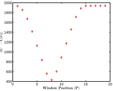
set at p= 1, a solution vector X(r) is obtained for the chosen aspect ratio. Then the forward problem is solved to obtain a CLD C(r) at that aspect ratio and window position p= 1. The window position is advanced one step forward and the calculation repeated until the last bin of the chord length histogram is reached. The window position at which the L2 norm

kC∗−C(r)k (25)

is minimized is the optimum window position for that window size. This optimum window then sets the particle size range to construct the optimum transformation matrix A˜ at that window size. The case of S = 20 applied to the CLD from Sample 1 (using the LW model) is shown in Fig. 5. The procedure is repeated using windows of different sizes and eventually the optimum window size and position which set the particle size range for the chosen aspect ratio is obtained. The whole process is repeated at different aspect ratios, and for each aspect ratio the particle size range is obtained from the optimum window size and position.

The key parameters of the algorithm are the quantitiesr,S,qandN. An extensive study (see section 2 of the supplementary information) has shown that a value ofN = 70 is suitable for the two models implemented here. The algorithm starts with an initial window size S after which the window size is increased. In section 2 of the supplementary information it was demonstrated that initial values of S from 2 up to 50 give consistent results for N _& 60. However an initial value of S = 6 was used in all the calculations here for more accuracy. The smallest value of q that can be used is q= 1, however a value of q = 2 was used here since there is no significant change in the level of accuracy obtained at q = 1. The value of q = 1 will only lead to greater resolution as can be seen in Fig. 5. Once the initial value of S, the values of q and N have been fixed, then the algorithm loops through subsequent values of S at all desired values of r as summarised below:

5_{The valuesq= 2, and initial window sizeS= 6 were used for both the VSM and LW}

0 5 10 15 20 400

600 800 1000 1200 1400 1600 1800 2000

Window Position(P)

k

C

*−

C

(

r

)

k

Figure 5: An example of the minimisation of theL2 norm in Eq. (25) when a window of

a given size approaches and passes its optimum position along the bin boundaries of the chord length histogram.

1. Choose an aspect ratio r.

2. Choose a number S of bins of the chord length histogram.

3. Start at window positionp= 1.

4. Obtain the values of Dmin and Dmax dictated by the window at the

position set by p.

5. Construct matrix ˜A corresponding to the values of Dmin and Dmax in

step 4.

6. Augment matrix ˜A with columns of ones and extend the particle size range as necessary.

7. Implement the LM algorithm to calculate γ starting with γ = 0, and then calculate X(r) from Eq. (22).

8. CalculateC(r) from Eq. (4).

9. Calculate theL2 norm in Eq. (25) for the given values of r, S and p.

11. Choose the best window position (the window position with the mini-mum L2 norm as in Fig. 5) for the given values of r and S.

12. Update the window size S and repeat steps 3 to 11.

13. For a given r obtain the window position and size at which the L2

norm in Eq. (25) attains its minimum. Record the particle size range corresponding to this window position and size.

14. Update r and repeat steps 2 to 13.

The values ofS used in the algorithm will depend on the desired level of accuracy. Using closely spaced values of S will result in greater accuracy but with the consequent increase in computational time. However widely spaced values of S will lead to lower computational times but less accurate results. The window sizes are calculated as

Sk=S0+

(k−1) M

Nw

, (26)

where b·cis the floor function discussed in Eq. (18),S0 is the initial window

size andNw < M is the desired number of windows. A value ofNw = 50 was

used in the calculations here. The values of r chosen depends on the desired range of aspect ratios to explore.

Having obtained the optimum particle size ranges at different aspect ra-tios for a particular sample, then the optimum aspect ratio for that sample can be chosen using a suitable procedure. The simplest procedure would have been to pick the aspect ratio at which the L2 norm reaches its global

minimum. However, the simulations show (see section 6 of supplementary information) that when the number of particle size bins is large enough the

L2 norm in Eq. (25) does not show a clear global minimum. Instead it

decreases with increasing aspect ratio and then levels off after some critical aspect ratio. Hence unique shape information cannot be obtained using the objective function in Eq. (24).

This problem of non uniqueness can be removed if the shape of the re-covered PSD (Xi in Eq. (24)) is taken into account. As the aspect ratio

To address this issue, one can introduce a modified function which reduces these oscillations by minimising the total variation in the PSD. Here we use a new objective function f2 given as

f2 = M X

j=1 "

C_j∗− N X

i=1

˜

AjiXi #2

+λ N X

i=1

X_i2, (27)

where the parameter λ sets the level of the penalty function imposed on the norm of the PSD. The value of λis chosen by comparing the relative magni-tude of the two sums of squares in Eq. (27) (see section 6 of supplementary information for more details). The optimum particle size ranges at differ-ent aspect ratios obtained using the inversion algorithm above are used to construct the transformation matrix ˜A (in Eq. (27)) at the corresponding aspect ratios. The optimum aspect ratio is chosen as the value of r at which the objective function f2 reaches its global minimum for a carefully chosen

value of λ. The corresponding PSD at which f2 reaches its global minimum

is then chosen as the optimum PSD.

For a meaningful comparison of calculated PSD with experimentally mea-sured PSD from laser diffraction and imaging, it is necessary that the cal-culated PSD be cast as a volume based distribution. This is because some instruments report PSD in terms of a volume based distribution for example Figs. 3(a), 3(b) and3(c). The volume based PSDXv given by [31]

X_iv = X

o iD

3 i

PN

i X o iD

3 i

, (28)

(whereXo is the optimum number based PSD which minimises the objective functionf2 in Eq. (27)) could lead to artificial peaks at large particle sizes if

there are small fluctuations in the right hand tail of the number based PSD estimates (see section 5 of supplementary information). These fluctuations are usually very small with an amplitude of the order of 0.1% of the peak of the number based PSD Xi in Eq. (27). Because the amplitude of the

as follows:

Calculate the CLD C_jo given by

C_jo = ˜Ao_jiXˆ_io, (29)

where ˜Ao

ji is the optimum transformation matrix obtained by the inversion

algorithm and

ˆ

X_io = X

o i

PN

i X o i

. (30)

If the volume based PSD Xv

i was known, then the CLD Cjo can also be

calculated from

C_jo =Ao_jiXv_i, (31)

where

Ao_ji = ˜

Ao_ji

D3_i

(32a)

X_iv = ˆ

Xo iD

3 i

PN

i Xˆ o iD

3 i

(32b)

Xv_i =

" _N X

i

X_ioD3_i #

X_iv. (32c)

Equation (31) is the forward problem for the volume based PSD similar to the case of Eq. (4) for the number based PSD. However, since the volume based PSD is not known, then an objective function similar to f2 in Eq. (27) can be formulated to recover the volume based PSD. This objective function

f3 is given as

f3 = M X

j=1 "

C_jo− N X

i=1

Ao_jiXv_i #2

+λ N X

i=1

Xv_i2. (33)

This allows Xv_i (obtained to some weighting factor due to Eq. (32)(c)) to be calculated as

Xv_i =eγiv, i= 1,2, . . . , N, (34)

where γv

i is an arbitrary parameter which is used to minimise the objective

0.05 0.1 0.15 0.2 0.25 0.3 0.35 0.4 20

50 100 500

rc

P j

[

C

*−j Cj

]

2+

λ

P i

X

2 i

1 2 3 4 5

0 0.1 0.2 0.3 0.4

Sample#

M

in

rc

0.2 0.4 0.6 0.8 1

103 104 105

re

P j

[

C

*−j Cj

]

2+

λ

P i

X

2 i

1 2 3 4 5

0 0.1 0.2 0.3 0.4

Sample#

M

in

re

(a) (c)

(d) (b)

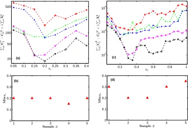
Figure 6: (a) The minimum values of the objective function in Eq. (27) versus the aspect ratio (the minimum values of the objective function for all window sizes and positions for each sample indicated with symbols as: Sample 1 - red pentagrams, Sample 2 - green crosses, Sample 3 - blue asterisks, Sample 4 - magenta squares, Sample 5 - black circles) obtained with the VSM model. (b) The aspect ratios (M in rc) at which the objective

func-tion reaches a global minimum for each Sample obtained with the VSM model. (c) Similar to (a) obtained with the LW model. (d) Similar to (b) with the LW model.

normalised and made grid independent as

˜

X_iv = X

v i

(Di+1−Di)PN_i X v i

. (35)

5. Results and Discussion

Once the optimum particle size ranges at the different aspect ratios have been obtained using the inversion algorithm, then the optimum aspect ratio for each sample can be determined by selecting the aspect ratio at which the objective functionf2 (in Eq. (27)) reaches its global minimum. The objective

1 is shown in Fig. 6(a) for the case of the VSM model6_{. The function f}

2

reaches its global minimum at rc ≈ 0.2 as in Fig. 6(b). The calculations

with the VSM model was restricted to the range rc ∈ [0,0.4] because the

thin cylindrical VSM model is only valid for rc1 [11].

Figure 6(c) shows a similar result to Fig. 6(a) for the same samples in Fig. 1 for the case of the LW model. The function f2 reaches its global minimum for re≈0.3 as in Fig. 6(d). In this case, the aspect ratiosre cover

a broader range re ∈ [0,1] since the LW model is valid for re ∈ [0,1]. The

aspect ratios predicted by the VSM and LW models in Figs. 6(b) and 6(d) are comparable to the aspect ratios estimated from image data in Fig. 3(d), although the calculated aspect ratios appear slightly higher.

The aspect ratios predicted by the VSM model in Fig. 6(b) are closer to the estimated aspect ratios in Fig. 3(d) when compared with the aspect ratios predicted by the LW model in Fig. 6(d). This could be because the cylindrical shape used in the VSM model is closer to the shape of the particles in Fig. 1 than the ellipsoidal shape used in the LW model. We also note that the VSM model gives much lower error norm than the LW model for the same aspect ratio as seen in Figs. 6(a) and 6(c), and this is also the case when λ= 0 (see section 6 of supplementary information). The effect of shape on the level of accuracy reached in the calculations is demonstrated by the fact that when the LW model is applied to a system of spherical particles (section 6 of supplementary information), the error norm obtained in that case is comparable to the error norm obtained when the VSM model is applied to the needle particles.

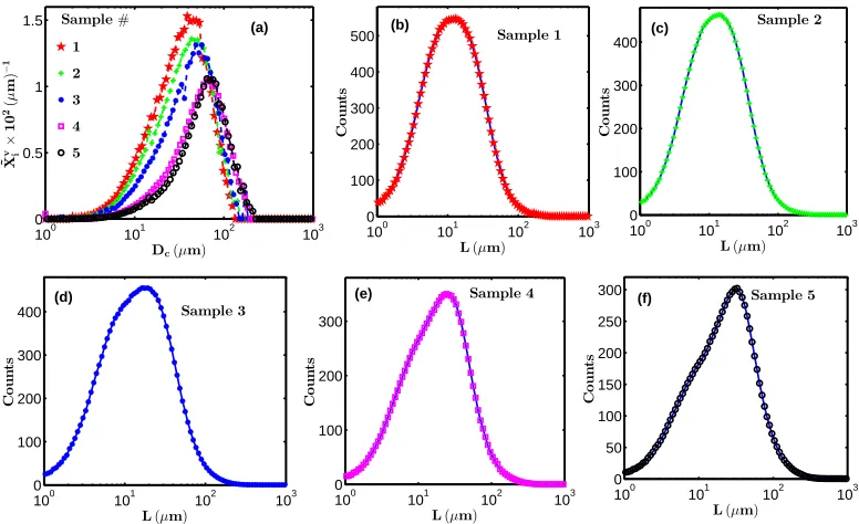
Figure 7(a) shows the recovered volume based PSD calculated by min-imising the objective functionf3 in Eq. (33) using the optimum aspect ratios

in Fig. 6(b)7 for the case of the VSM model. The transformation matrix ˜Ao

used in Eq. (32) was constructed using the optimum particle size range ob-tained by the inversion algorithm and aspect ratios shown in Fig. 6(b). The matrix ˜Ao is then weighted as in Eq. (32)(a) to obtain the matrix Ao. The volume based PSD ˜Xv _{normalised and rescaled as in Eq. (35) are shown in}

Fig. 7(a).

The PSDs in Fig. 7(a) are shown as a function of the characteristic

6_{The values ofλ= 0.01 andλ= 0.2 were used in Eq. (26) for the VSM and LW model}

respectively (section 6 of the supplementary information)

7_{The values of λ= 0 andλ= 8×10}−15 _{were used in Eq. (33) for the VSM and LW}

100 101 102 103 0

0.5 1 1.5

Dc(µm)

˜ X

v×i

1 0 2( µ m ) − 1 Sample# 1 2 3 4 5

100 101 102 103 0 100 200 300 400 500

L(µm)

C o u n ts Sample 1

100 101 102 103 0

100 200 300 400

L(µm)

C o u n ts Sample 2

100 101 102 103 0

100 200 300 400

L(µm)

C o u n ts Sample 3

100 101 102 103 0

100 200 300

L(µm)

C o u n ts Sample 4

100 101 102 103 0 50 100 150 200 250 300

L(µm)

C o u n ts Sample 5

(a) (b) (c)

(d) (e) (f)

Figure 7: (a) The recovered volume based PSDs calculated from the objective function in Eq. (33) for λ = 0 (with the VSM model) at the minimum aspect ratios (shown in Fig. 6(b)) for each Sample. (b)-(f) Calculated (symbols) and measured (solid line) Chord Length Distributions for the Samples indicated in each Figure. The calculated CLDs were obtained by solving the forward problem in Eq. (4) using the number based PSD which minimise the objective function in Eq. (23) forλ= 0.01.

particle sizeDc. This PSD can be compared to the data from laser diffraction

in Fig. 2(a) and EQPC diameter in Fig. 3(a). The particle sizes in Fig. 7(a) cover a range of Dc ≈7µm to Dc≈ 200µm. The modes of the distributions

cover a range of Dc ≈ 40µm to Dc ≈ 70µm, with the sizes increasing from

sample 1 to sample 5. This is consistent with the data from laser diffraction in Fig. 2(a) where the diameters cover a range of about 2µm to about 200µm. The modes of the distributions cover a range of about 10µm to about 30µm with the particle sizes increasing from sample 1 to sample 5. Similarly, the EQPC diameters in Fig. 3(a) cover a range of about 10µm to about 200µm with the modes running from about 30µm to about 100µm, and the sizes increasing from sample 1 to sample 5. The peaks of the PSDs from the laser diffraction in Fig. 2(a) and EQPC diameters in Fig. 3(a) decrease from sample 1 to sample 5 which is consistent with the results reported in Fig.

The symbols in Figs. 7(b) to 7(f) show the calculated (using the VSM model) CLDs for the five samples in Fig. 1. The CLDs were calculated from Eq. (4) using the number based PSD which minimises the objective function

f2 in Eq. (27). The calculations were done at the optimum aspect ratios in

Fig. 6(b). The blue solid lines in Figs. 7(b) to 7(f) are the experimentally measured CLDs for the five samples shown in Fig. 2(b). The agreement between the calculated CLDs and the experimentally measured CLDs in Figs. 7(b) to 7(f) is near perfect. This level of agreement between the calculated PSD and CLD with the experimentally measured PSD and CLD demonstrates the level of accuracy that can be achieved with this algorithm.

100 101 102 103 0

0.5 1 1.5 2

De(µm) ˜ X

v×i

1 0 2( µ m ) − 1 Sample# 1 2 3 4 5

100 101 102 103 0 100 200 300 400 500

L(µm)

C o u n ts (b)

100 101 102 103 0

100 200 300 400

L(µm)

C o u n ts Sample 2

100 101 102 103 0

100 200 300 400

L(µm)

C o u n ts Sample 3

100 101 102 103 0

100 200 300

L(µm)

C o u n ts Sample 4

100 101 102 103 0 50 100 150 200 250 300

L(µm)

C o u n ts Sample 5 (a)

(d) (e) (f)

(c) (b)

Figure 8: Similar to Fig. 7obtained with the LW model. In this case the volume weighted PSDs were obtained at λ= 10−14 _{from Eq.(33), while the CLDs correspond to number}

based PSD obtained atλ= 0.2 from Eq. (27).

Figure 8(a) shows the volume based PSDs for the five samples in Fig.

1 calculated with the LW model. The calculations were done in a similar manner as in Fig. 7(a). The distributions are plotted as a function of the characteristic size De which are comparable to the laser diffraction data in

100 101 102 103 0

0.2 0.4 0.6 0.8 1

lc=ac(µm)

˜ X v×i

1

0

2(

µ

m

)

−

1

Sample#

1

2

3

4

5

100 101 102 103

0 0.2 0.4 0.6 0.8 1 1.2

le=2ae(µm)

˜ X v×i

1

0

2(

µ

m

)

−

1

(a) (b)

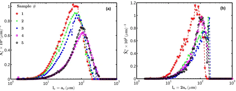
Figure 9: Particle lengths for the five samples calculated with (a) the VSM model and (b) the LW model.

similar to the case of Fig. 7(a). The range of particle sizes in Fig. 8(a) and the modes of the distributions in Fig. 8(a) are close to the measured data in Figs. 2(a) and 3(a). However, the calculated PSDs in Fig. 8(a) show some oscillations. This is also reflected in the fact that the error norms between the measured CLD and calculated CLD with the LW model is higher than the corresponding error norm of the calculations with the VSM model as seen in Figs. 6(a) and 6(c).

The symbols in Figs. 8(b) to 8(f) show the calculated (using the LW model) CLDs for the samples in Fig. 1. The calculations were done in a manner similar to the case of Figs. 7(b) to 7(f). However, the calculated CLDs in Figs. 8(b) to 8(f) show a slight mismatch with the experimental data unlike the case of Figs. 7(b) to 7(f) where the match is near perfect.

A likely reason for the different levels of agreement between calculated data with the two models and experimental data is that different kinds of approximations were made in the formulation of the models. The VSM model considers all possible 3 D orientations of the cylinder in the computation of the cylindrical PDF [11]. However, the LW model considers only one 2 D projection of the ellipsoid where the major and minor axes are parallel to the x−y plane [9]. Also, the cylindrical shape of the VSM model is closer to the needle shape of the particles than the ellipsoidal shape of the LW.

Figure9(a) shows the volume based PSD calculated with the VSM model plotted as a function of the characteristic length lc = ac (the length of the

samples 4 and 5, and about 10µm to about 500µm for samples 1 to 3. The characteristic lengths predicted by the VSM model in Fig. 9(a) are short of the Feret Max data in Fig. 3(b) because the aspect ratios predicted by the VSM model in Fig. 6(b) are higher than the estimated aspect ratios in Fig.

3(d). This implies that the VSM model predicts needles that are slightly thicker and shorter than the actual needles in the samples. However, the needle lengths calculated with the VSM model cover a range of about 10µm to about 300µm which are still comparable to the Feret max measurements in Fig. 3(b).

A similar situation holds for the LW model where the predicted ellipsoid heights (le in Fig. 9(b)) are short of the Feret Max measurements in Fig. 3(b). Similarly, the aspect ratios predicted by the LW model in Fig. 6(d) are higher than the estimated aspect ratios in Fig. 3(d). This again shows that the LW model predicts needles which are slightly thicker and shorter than the actual needles in the samples. The range of needle lengths calculated with the LW model are reasonable when compared with the measured Feret Max in Fig. 3(b).

Even though the predicted lengths (lcandle) do not have a perfect match

with the measured Feret Max data, the trend in the lengths of needles from sample 1 to sample 5 in Fig. 3(b) are consistent with the trend in needle lengths from sample 1 to sample 5 in Fig. 9(a). However, the trend in needle lengths in Fig. 9(b) are not so consistent with the trend in needle lengths in Fig. 3(b) moving from sample 1 to sample 5. This is because the LW model predicts smaller aspect ratios for sample 2 and sample 3 in Fig. 6(d) resulting in a shift of the distributions to higher values for sample 2 and sample 3 in Fig. 9(b).

6. Conclusions

properties. In the case considered here the particles were treated as opaque and assumed to have convex shapes (that is cylindrical or ellipsoidal). This representation is suitable for the CoA particles considered here as can be seen in Fig. 1. A more detailed discussion of the possible errors that can occur from using this representation is presented in Section 8 of the supplementary information. Also in the supplementary information is a detailed analysis of sensitivity of resulting estimates to choice of algorithm parameters to validate accuracy and robustness of algorithm outcomes.

We applied the algorithm to previously collected CLD data for slurries of needle shaped crystalline particles of COA with different particle size distri-butions. COA slurries were characterised using FBRM (to measure CLD), imaging (to measure EQPC, maximum and minimum Feret diameters) and laser diffraction (to measure PSD based on equivalent sphere diameter ap-proximation). Measured CLD data were used in the algorithm without any further information input, using two different CLD geometrical models, one for ellipsoids and the other one for thin cylinders. Best estimates for particle aspect ratios and corresponding PSDs were obtained with each model and these were compared to experimental data from imaging and laser diffraction. Estimated aspect ratios from the thin cylinder model were in good agree-ment with those obtained from the ratio of maximum and minimum Feret diameters, while those from the ellipsoid model were somewhat higher. Cor-responding to this, there was a good agreement between measured and fitted CLDs for the thin cylinder model, but some discrepancies could be seen for the ellipsoid model. Ranges and modes of particle size distributions deter-mined for both models were in a good agreement with those obtained by imaging. Although it was possible to estimate aspect ratios of needle like particles from CLD data reasonably accurately for the system analysed here, the optimisation problem of finding most appropriate PSD and aspect ra-tio would be greatly simplified if addira-tional informara-tion about particle size range or shape is available, for example from a suitable imaging or scattering technique, especially in the case of systems with significant polydispersity or multimodality in terms of particle shape or size.

Acknowledgement

Supplementary Information

1. Slack Variables

The concept of slack variables in optimisation problems is described in previous literature [29]. The idea of introducing columns of 1s to the transfor-mation matrix is based on the following argument. Consider the optimisation problem:

find β which minimises the objective function φ where

φ=

M X

i=1

[yi−gi(β)]2, (1)

where y ∈ _RM_{, β ∈}

RN and g : RN → R. The optimisation problem in Eq.

(1) is equivalent to

minimise

M X

i=1 zi

subject to zi = [yi−gi(β)] 2

.

(2)

Since [yi−gi(β)]2 ≥0, then zi ≥yi−gi(β). Hence the optimisation problem

in Eq. (2) is equivalent to

minimise

M X

i=1 zi

subject to yi−gi(β)−zi ≤0.

(3)

There exist slack variablessi ≥0, j = 1,2, . . . , M such that yi−gi(β)−zi+ si = 0. Hence the optimisation problem in Eq. (3) is equivalent to

minimise

M X

i=1 zi

subject to yi−gi(β)−zi+si = 0 si ≥0.

Substituting for zi in Eq. (4) gives the following equivalent formulation for

the optimisation problem in Eq. (1):

minimise

M X

i=1

yi−gi(β) +si

subject to si ≥0 .

(5)

2. Choice of Algorithm Parameters

10 20 30 40 50 60 70 80

0 50 100 150 200 250 300

N

k

C

*−

C

(

r

)

k

re=0_.1 re=0_.3

re=0_.5 re=0_.7

100 101 102 103

0 20 40 60 80 100

De

C

o

u

n

t

s

re=0_.3 N=20 N=40 N=60 N=80

100 101 102 103

0 100 200 300 400 500 600

L

C

o

u

n

t

s

re=0_.3

N=20 N=40

N=60

N=80

(a) (b)

(c)

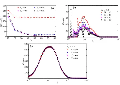
Figure 1: (a) Variation of theL2 norm in Eq. 25 of the main text (from the LW model)

with the number of size binsN at the different aspect ratiosre(indicated in the Figure) for

Sample 1. (b) Recovered number distributed PSDs (from the LW model) at the specified values ofreandN. The quantityDeis the characteristic size for the LW model described

in the main text. (c) Chord length distributions corresponding to the PSDs in (b). The parameterLis the chord length described in the main text.

10 20 30 40 50 60 70 80 0

200 400 600 800

N

k

C

*−

C

(

r

)

k

rc=0_.1 rc=0_.2

rc=0_.3 rc=0_.4

100 101 102 103

0 20 40 60 80

Dc

C

o

u

n

t

s

rc=0_.3

N=20

N=40

N=60

N=80

100 101 102 103

0 100 200 300 400 500 600

L

C

o

u

n

t

s

rc=0_.3

N=20 N=40 N=60 N=80

(a) (b)

(c)

Figure 2: Similar to Fig. 1obtained with the VSM model.

2.1. Number of size bins N

The solution vector X which minimises the objective function f1 in Eq.

(24) of the main text varies slightly with different numbers of particle size bins N. This in turn leads to a variation in the vector C obtained from the forward problem in Eq. (4) of the main text. Hence different values of

N were used and each time the L2 norm in Eq. (25) of the main text was

calculated in order to determine the optimum number of fitting parameters. The variation of the L2 norm with the number of particle size bins N at

different aspect ratios for the LW model is shown in Fig. 1(a). As the value of N increases, theL2 norm decreases gradually and then begins to level off

at large values ofN. The result is the same for different aspect ratiosre as in

Fig. 1(a). For a fixed aspect ratio re (for examplere = 0.3 in Fig. 1(b)) and

100 101 102 103 0

10 20 30 40 50 60 70

De

C

o

u

n

t

s

re=0.1

re=0.3

re=0.5

re=0.7

100 101 102 103

0 10 20 30 40 50 60 70

De

C

o

u

n

t

s

re=0.1

re=0.3

re=0.5

re=0.7

100 101 102 103

0 10 20 30 40 50 60 70

De

C

o

u

n

t

s

re=0.1

re=0.3

re=0.5

re=0.7

(a) _(b)

(c) N=60, LW

N=70,LW

N=80,LW

Figure 3: Particle size distributions recovered (using the LW model at the aspect ratios reindicated) by minimising the objective function f1 in the main text using the different

number of particle size bins N indicated in each figure.

Fig. 1(b). However, the oscillations in the corresponding CLD decrease as in Fig. 1(c). As N is increased further, the oscillations in the recovered PSD become more severe as in Fig. 1(b) for N = 80. The corresponding CLD for

N = 80 shows very little change from that obtained at N = 40.

A similar situation holds for the VSM model where theL2 norm levels off

with increasingN as in Fig. 2(a) for different aspect ratiosrc. The behaviour

of the recovered PSDs for different values of N in Fig. 2(b) is similar to the case of Fig. 1(b). Also, the behaviour of the corresponding CLDs for different values of N in Fig. 2(c) is similar to the case of Fig. 1(c).

100 101 102 103 0

10 20 30 40 50

Dc

C

o

u

n

t

s

rc=0.1

rc₌0

.2

rc=0.3

rc₌0_.4

100 101 102 103

0 10 20 30 40 50

Dc

C

o

u

n

t

s

rc=0.1

rc₌0_.2

rc₌0

.3

rc=0.4

100 101 102 103

0 10 20 30 40 50 60

Dc

C

o

u

n

t

s

rc=0.1

rc₌0

.2

rc=0.3

rc₌0_.4

N=60, VSM

N=70, VSM

N=80, VSM

(c)

(a) (b)

Figure 4: Same as in Fig. 3 with the VSM model.

more clearly in Figs. 3 and 4.

Figure 3(a) shows the recovered PSD (with the LW model) at the indi-cated aspect ratios re for N = 60. The PSD for re = 0.1 is fairly smooth

except the long spike atDe≈1. However, the PSDs begin to develop

oscilla-tions as the aspect ratiore increases as seen in the cases ofre = [0.3,0.5,0.7]

in Fig. 3(a). A similar situation holds for N = 70 (Fig. 3(b)) and N = 80 (Fig. 3(c)). However, the oscillations for the case of N = 80 is much more severe.

Figure4 is similar to Fig. 3 but calculated with the VSM model. For a fixed N, the fluctuations in the PSDs increase as the aspect ratiorc increases

as seen in Figs. 4(a), 4(b) and 4(c). The level of fluctuations at N = 80 in Fig. 4(c) is much more severe when compared with the cases ofN = 60 (Fig.

4(a)) and N = 70 (Fig. 4(b)). For N = 60 (Fig. 4(a)) the small particle sizes of Dc ≈ 2 for rc >0.1 are not fully resolved when compared with the

10 20 30 40 50 50

100 150 200 250

S0

k

C

*−

C

(

r

)

k N=20,LW

re=0.1

re=0.3

re=0.5

re=0.7

10 20 30 40 50

0 50 100 150 200

S0

k

C

*−

C

(

r

)

k

N=40,LW

re=0.1

re=0.3

re=0.5

re=0.7

10 20 30 40 50

0 50 100 150 200

S0

k

C

*−

C

(

r

)

k

N=60,LW

re=0.1

re=0.3

re=0.5

re=0.7

(a)

(b) (c)

Figure 5: Variation of theL2norm in Eq. 25 of the main text with different initial values

of window sizeSw. The calculations were done with the LW model at the different aspect

ratiosreand number of particle size bins N indicated in each figure.

of accuracy in the calculations does not increase significantly for N > 70. Instead, using a larger value of N only leads to severe fluctuations in the calculated PSDs and longer computational times. The value of N = 70 also gives a better resolution of small particle sizes for both models. Hence a value of N = 70 was used in all the calculations in the main text.

2.2. Window size S and spacing q

The inversion algorithm described in Section 4 of the main text places a window of size S on the bins of the chord length histogram. This win-dow starts with an initial size S0, then slides along the bins of the chord

10 20 30 40 50 400

450 500 550 600 650

S0

k

C

*−

C

(

r

)

k

N₌20,VSM

rc=0.1

rc=0.3

10 20 30 40 50

55 60 65 70 75 80 85

S0

k

C

*−

C

(

r

)

k

rc=0.1

rc=0.3

N₌40,VSM

10 20 30 40 50

0 5 10 15 20 25

S0

k

C

*−

C

(

r

)

k rc=0.1

rc=0.3

N=60,VSM

(a)

(b)

(c)

Figure 6: Same as in Fig. 5 with the VSM model.

appropriate number of size bins at which the accuracy of the calculations become independent of the initial window size?

Figure 5(a) shows that for N = 20 (calculations with the LW model), the L2 norm in Eq. 25 of the main text (calculated at the optimum window

size and position) shows a dependence on S0 at different aspect ratios. This

dependence reduces significantly at N = 40 as in Fig. 5(b) and becomes nearly independent at N = 60.

A similar situation holds for calculations with the VSM model where the large dependence of the L2 norm (at different aspect ratios) on S0 seen in

Fig. 6(a) (for N = 20) decreases as N increases to 40 in Fig. 6(b). The

L2 norm becomes nearly independent of S0 at N = 60 as in Fig. 6(c). The

values of the L2 norm obtained with the VSM model for N & 40 (Fig. 6)

are significantly less than the values of the L2 norm obtained with the LW

geometry of the LW for sufficiently large N.

The results in Figs. 5 and 6 suggest that any value of S0 from 2 up

to 50 (corresponding to a particle size range of about 1µm to about 43µm) could be used in the calculations for N _& 60. However, a value of S0 = 6

(corresponding to a particle size range of 1µm to 1.5µm) and N = 70 were used in all the calculations in the main text. The spacing between consecutive positions (that is, q in Eq. 17 of the main text) was kept at q= 2 in all the calculations in the main text. The smallest value of q = 1 did not yield any significant increase in accuracy of the calculations.

3. Length Weighting

In this section we present a simple numerical simulation which demon-strates the effect of particle size on detection probability. It had already been suggested [11,19,20] that larger particles have a higher probability of being encountered by the FBRM laser. Here we represent the laser beam in the focal plane by the red circle in Fig. 7(a). The circular window of the probe is represented by the black circle in Fig. 7(a). We simulate spherical particles (represented by the blue circles in Fig. 7(a)) falling at random positions on the plane of the laser spot. We assume that all particles regardless of size have equal probability of falling in the focal plane. Each time the boundary of a particle intersects the trajectory of the laser beam a ‘hit’ is recorded. The idea behind the simulation is to see how the number of hits scales with the particle size (diameter of each circle).

Since each event of a particle falling on the focal plane is independent of another particle falling on the focal plane, then we simulate Nr realisations

of a single particle of size Ds falling on the focal plane separately from the

same number of realisations of another particle of a different size.

The FBRM probe reports chord lengths between 1µm and 1000µm (for example Fig. 2(b) of the main text). Hence we set the particles sizes Ds ∈

[10−3_{,1]mm. The radius R}

L of the laser beam is set at 4 mm [2], while the

radius of the circular window RW is set in multiples of RL.

0 0.2 0.4 0.6 0.8 1 0

0.5 1 1.5

2x 10

5

Ds(mm)

H

it

s

RW=2RL

RW=4RL

RW=6RL

RW=8RL

RW=10RL

(a)

R

W

R_L

D_s

(b)

Figure 7: (a) Pictorial representation of the viewing window (black circle) of the FBRM probe, the laser beam (in the focal plane) is represented by the red circle while spherical particles are represented by the blue circles. (b) Variation of the frequencies of hits of the laser beam with different particles of sizesDsand different sizes of the viewing window as

indicated in the Figure.

4. Single Particle and Population CLD

In this section we show the single particle CLD realised with the LW and VSM models. Then we demonstrate the effect of length weighting on the population CLD.

4.1. Single Particle CLD of LW and VSM models

Different mathematical approximations were made in the formulation of the LW and VSM models [9, 11] as already noted in the main text. These different approximations give rise to different CLDs for a single particle of similar geometrical shape. The single particle CLDs (for different aspect ratios) realised for an ellipsoid (an ellipse in 2D) of length le = 2ae = 100µm

(ae is the length of the semi major axis) is shown in Fig. 8(a). The peaks of

the single particle CLDs shift to the left as the aspect ratiore=be/ae(where beis the semi minor axis length) is decreased. The single particle CLDs of the

LW model increase slowly at small chord lengths before reaching their peaks at 2be and then decrease to zero at le. They have a right shoulder which gets

broader as re is decreased. The LW model approximates the single particle

100 101 102 103 0

0.05 0.1

Particle Size

X

s,

X

t

100 101 102 103

0 0.01 0.02 0.03 0.04 0.05

Chord length

C

5 10

C

+

C+

C

100 101 102 103

0 0.1 0.2 0.3 0.4

Chord length

C

L

D

LW,re=0.1

LW,re=0.2

LW,re=0.3

VSM,rc=0.1

VSM,rc=0.2

VSM,rc=0.3

10 20 30

X

f

Xs

Xt

Xf

(a)

(b)

(c)

Figure 8: (a) Single particle CLDs for an ellipsoid (for the LW model with aspect ratios indicated asre) of lengthle= 2ae= 100µm (ae= semi major axis length of ellipsoid) and

a cylinder (for the VSM model with aspect ratios indicated as rc) of heightac = 100µm.

(b) Simulated PSDXs_{, recovered PSDsX}t_{(with length weighted transformation matrix)}

and Xf (with unweighted transformation matrix). (c) Weighted CLD C+ from Xs due to weighted transformation matrix and unweigthed CLD C fromXs due to unweighted transformation matrix.

what the effects of the other orientations of the ellipsoid will have on the single particle CLD as these orientations were not considered.

The single particle CLDs of the cylindrical (for a cylinder of height

ac = 100µm) VSM model shown in Fig. 8(a) are less sensitive to small

chord lengths as they rise very quickly to their peaks at 2bc (bc is the radius

of the cylinder). They then decrease more slowly (in a manner similar to the LW case) to zero at ac. The low sensitivity of the single particle cylindrical

cylindrical VSM match those of the LW for the same aspect ratio as seen in Fig. 8(a).

4.2. Effect of Length Weighting on Population CLD and Recovered PSD

The effect of the size of a particle to its detection probability has been demonstrated in section3. This length bias could have a substantial effect on the calculations if it is not incorporated in some way. Consider the simulated PSDXsshown by the solid line in Fig. 8(b). The PSD was made by randomly drawing 106_{particle sizes from the normal distribution with mean size 500µm}

and standard deviation 100µm. Then the particle sizes were shifted to ensure non negativity. Finally the PSD was made from a normalised histogram of 30 bins. The solid line in Fig. 8(c) shows the CLD C calculated from the normalised PSD Xs _as

C =AXs, (6)

where A8 _{is the transformation matrix in Eq. (6) of the main text without}

any length weighting. The symbols in Fig. 8(c) show the CLDC+calculated from the normalised PSD Xs _as

C+=AX˜ s, (7)

whereA˜ is the transformation matrix in Eq. (5) of the main text with length weighting. Figure8(c) shows that the CLDC+_{calculated with length}

weight-ing is substantially higher than the correspondweight-ing CLD C without length weighting and slightly shifted to the right. This shows that the experimen-tally measured CLD could be substantially biased due to the length weighting effect demonstrated in section 3. Hence the length weighting effect needs to be incorporated into the calculations to account for this length bias.

The red diamonds in Fig. 8(b) show the PSD obtained by minimising the objective function φ (similar to the function f1 in Eq. 24 of the main text)

given as

φ =

M X

j=1 "

C_j+− N X

i=1

˜

AjiXit #2

, (8)

whereM is the number of chord length bins,N is the number of particle size bins and Xt _{is the optimum PSD which minimises the objective function.}

The recovered PSD Xt _{matches the original PSD X}s _{because the length}

weighting effect has been incorporated into the matrix A˜. However, when the objective function is formulated as

φ=

M X

j=1 "

C_j+− N X

i=1 AjiX

f i

#2

, (9)

the optimum PSD Xf is substantially higher than the original PSD Xs and slightly shifted to the right as seen in Fig. 8(b). This again demonstrates the need to account for the length bias that comes with the experimentally measured CLD to reduce its effect on the calculated PSD.

5. Number and Volume Based PSD

Some particle sizing instruments report the PSD in terms of a volume distribution for example Figs. 2(a), 3(a), 3(b) and 3(c) of the main text. Hence it becomes necessary to calculate a volume based PSD that is compa-rable to the experimentally measured PSDs. The volume based PSD Xv can be calculated from [31]

X_iv = XiD

3 i

PN

i=1XiD 3 i

, (10)

where X is the number based PSD and D is the characteristic size of the population of particles. This is equivalent to

X_iv = XˆiD

3 i

PN

i=1XˆiD 3 i

, (11)

where

ˆ

Xi = Xi

PN

i=1Xi

. (12)

100 101 102 103 0

0.02 0.04 0.06 0.08 0.1 0.12 0.14 0.16

De

P

S

D

Sample 1

X

Xv

1

Xv

2

re=0.3

100 101 102 103

0 0.01 0.02 0.03 0.04 0.05 0.06 0.07

Dc

P

S

D

Sample 1

X

Xv

1

Xv

2

rc=0.2

100 101 102 103

0 0.02 0.04 0.06 0.08 0.1 0.12

Particle Size

P

S

D

Xs

Xv

1

Xv

2

Simulated data

(c) (b)

(a)

Figure 9: (a) The simulated PSDXsin Fig. 8(b), volume based PSDsXv₁(calculated from Eq. (10) usingXs) andXv₂(calculated from Eq. (13)). (b) Normalised number based PSD

X obtained by minimising the function f1 in the main text using the LW model at the

aspect ratiore indicated in the figure. Volume based PSD Xv1 calculated from Eq. (10)

using the PSD X. Normalised volume based PSDXv2 obtained from the functionf3 (at

λ= 0) in the main text. (c) Same as in (b) with the VSM model.

fluctuation at De ≈ 200µm. This leads to the peak at De ≈ 200µm in

the volume based PSD Xv₁ calculated from Eq. (10). This peak is clearly artificial as the number based PSDX in Fig. 9(b) shows a near zero particle size count at De ≈ 200µm. This problem led to the formulation of a new

method for calculating the volume based PSD which allows the application of a suitable regularisation to remove these artificial peaks.

To demonstrate that the method summarised in Eqs. 29 to 33 of the main text reproduces the correct volume based PSD, consider the simulated PSD

Xs _{in Fig. 9(a) which is the same normalised PSD X}s _{in Fig. 8(b). The}

red squares in Fig. 9(a) show the volume based PSD Xv

1 calculated froom

Eq. (10) using the PSD Xs. The black pentagrams in Fig. 9(a) show the normalised volume based PSD Xv