Stabilization of hybrid systems by feedback control based on discrete-time state and mode observations

–Regular Paper–

STABILIZATION OF HYBRID SYSTEMS BY FEEDBACK CONTROL

BASED ON DISCRETE-TIME STATE AND MODE OBSERVATIONS

Jianqiu Lu1∗_{, Yuyuan Li}2_{, Xuerong Mao}1_{, Qinwei Qiu}2

ABSTRACT

Recently, Mao [1] proposed a kind of feedback control based on discrete-time state observations to stabilize continuous-discrete-time hybrid stochastic systems in mean-square sense. We find that the feedback control there still depends on the continuous-time observations of the mode. However, it usually costs to identify the current mode of the system in practice. So we can further improve the control to reduce the control cost by identifying the mode at discrete times when we make observations for the state. In this paper, we aim to design such a type of feedback controls based on the discrete-time observations of both state and mode to stabilize the given unstable hybrid stochastic differential equations (SDEs) in the sense of mean-square exponential stability. Moreover,

a numerical example isgiven to illustrate our results.

Key Words: Brownian motion, Markov chain, mean-square exponential stability, discrete-time feedback control.

1. INTRODUCTION

Hybrid stochastic differential equations (SDEs) (also known as SDEs with Markovian switching), usually used to model practical systems where they may experience abrupt changes in their structure and parameters, have been attracting a lot of attention in recent years. Particularly, as the most fundamental problem in engineering, the asymptotic stability has been studied extensively [2,3,4,6,12,13,14,18,20,

21,22,23,24,26,27,28,29,30]. Here we mention that [10,11] are two of the most cited papers while [17] is the first book in this area.

One classical topic in this field is the problem of stabilization, i.e. designing a control function

u(x(t), r(t), t) which usually appears in the drift part

∗_{Manuscript received 11 February 2016 and accepted on 8}

February 2017.

∗_{The authors are with} 1

Department of Mathematics and Statistics, University of Strathclyde, Glasgow G1 1XH, U.K.

2 _{College of Information Sciences and Technology, Donghua}

Univerisity, Shanghai 201620, China.

∗_{Jianqiu Lu (corresponding author, e-mail:}

[email protected]).

such that the controlled system

dx(t) =[f(x(t), r(t), t) +u(x(t), r(t), t)]dt

+ g(x(t), r(t), t)dw(t) (1.1)

will be stable though the original system (1.1) with

u(x(t), r(t), t) = 0 is unstable, where t≥0, r(t) is a Markov chain, x(t)∈Rn _{is the state, w(t) =}

(w1(t),· · · , wm(t))T is an m-dimensional Brownian

motion and the SDE is in the Itˆo sense.

Wang et al. in [25] designed a state feedback controller to stabilize bilinear uncertain time-delay stochastic systems with Markovian jumping parameters in mean square sense. In [5], the problem of almost sure exponential stabilization of stochastic systems by state-feedback controls was discussed. A robust delayed-state-feedback controller that exponentially stabilizes uncertain stochastic systems was proposed in [15]. It is observed that the state feedback controllers in these papers require continuous observations of the system state x(t) for all time t≥t0. Recently, Mao [1] first proposed to design a discrete-time feedback control

system

dx(t) =[f(x(t), r(t), t) +u(x(δ(t, t0, τ)), r(t), t)]dt

+g(x(t), r(t), t)dw(t)

(1.2)

become exponentially stable in mean square. Hereτ > 0is a constant and

δ(t, t0, τ) =t0+ [(t−t0)/τ]τ, (1.3)

in which [(t−t0)/τ] is the integer part of(t−t0)/τ.

The advantage of such a discrete-time feedback control is that it requires only state observations x(t0+kτ)

at discrete times t0, t0+τ, t0+ 2τ,· · · and hence it will cost much less and more realistic. Despite this advantage, we can take a further step to make it even better. We observe that the feedback control in Mao [1] is based on the discrete-time observations of the state x(t0+kτ)(k= 0,1,2,· · ·) but still depends on the continuous-time observations of the mode r(t)on

t≥t0. This is perfectly fine if the mode of the system can be fully observed at no cost. However, it usually costs to identify the current mode of the system in practice. So we can further improve the control to reduce the control cost by identifying the mode at discrete times when we make observations for the state. Therefore, in this paper, we will consider an n -dimensional controlled hybrid system

dx(t) =[f(x(t), r(t), t)

+u(x(δ(t, t0, τ)), r(δ(t, t0, τ), t)]dt

+g(x(t), r(t), t)dw(t)

(1.4)

ont≥t0, where our new feedback control is based on the discrete observations of statex(t0+kτ)and mode

r(t0+kτ).

Due to the difficulties arisen from the discrete-time Markov chainr(t0+kτ), the analysis in this paper will be much more complicated in comparison with the related previous papers and new techniques will be developed. Our main results will be formed in Section 3 and Sections 4 after giving preliminaries in Section 2. We will discuss an example in Section 5 to verify the effectiveness of the results and conclude our paper in Section 6.

2. Notation and Problem Statement

In this paper, we use the following notation. Let

(Ω,F,{Ft}t≥0,P)be a complete probability space with a filtration{Ft}t≥0satisfying the usual conditions (i.e.

it is increasing and right continuous withF0 contains

all P-null sets). Let w(t) = (w1(t),· · · , wm(t))T be an m-dimensional Brownian motion defined on the probability space. If A is a vector or matrix, its transpose is denoted by AT_{. If x∈R}n_{, then |x| is} its Euclidean norm. If A is a matrix, we let |A|=

p

trace(AT_{A)be its trace norm andkAk= max{|Ax|:} |x|= 1} be the operator norm. If A is a symmetric matrix (A=AT_{), denote byλ}

min(A)andλmax(A)its

smallest and largest eigenvalue, respectively. ByA≤0

and A <0, we mean A is non-positive and negative definite, respectively. Denote byL2

Ft(R

n_{)the family of}

allFt-measurable Rn-valued random variables ξsuch thatE|ξ|2<∞, whereEis the expectation with respect to the probability measureP.

Letr(t),t≥0, be a right-continuous Markov chain on the probability space taking values in a finite state spaceS ={1,2,· · · , N}with generatorΓ = (γij)N×N given by

P{r(t+ ∆) =j|r(t) =i}

=

(

γij∆ +o(∆) ifi6=j,

1 +γii∆ +o(∆) ifi=j,

where∆>0. Hereγij ≥0is the transition rate fromi tojifi6=jwhile

γii=− X

j6=i

γij.

We assume that the Markov chainr(·)is independent of the Brownian motionw(·). It is known that almost all sample paths ofr(t)are piecewise constant except for a finite number of simple jumps in any finite subinterval of R+ (:= [0,∞)). We stress that almost all sample

paths ofr(t)are right continuous.

Consider an n-dimensional uncontrolledunstable linear hybrid SDE

dx(t) =A(r(t))x(t)dt+

m X

k=1

Bk(r(t))x(t)dwk(t)

(2.1) ont≥0, with initial datax(0) =x0∈L2_F

0(R n₎

. Here

A, Bk :S→Rn×n and we will often write A(i) =

Ai and Bk(i) =Bki. Now we are required to design a feedback control u(x(δ(t)), r(δ(t))) based on the discrete-time state and mode observations in the drift part so that the controlledlinearSDE

dx(t) =[A(r(t))x(t) +u(x(δ(t)), r(δ(t)))]dt

+

m X

k=1

Bk(r(t))x(t)dwk(t)

(2.2)

c

will be mean-square exponentially stable, whereuis a mapping fromRn_×StoRn_{,τ >0and}

δ(t) = [t/τ]τ fort≥0, (2.3)

in which[t/τ]is the integer part oft/τ. As the given SDE (2.1) is linear, it is natural to use a linear feedback control. One of the most common linear feedback controls is the structure control of the formu(x, i) = F(i)G(i)x, where F and G are mappings from S to

Rn×landRl×n, respectively, and one of them is given while the other needs to be designed. These two cases are known as:

• State feedback: designF(·)whenG(·)is given; • Output injection: designG(·)whenF(·)is given.

Again, we will often write F(i) =Fi and G(i) =Gi. Then the controlled system (2.2) becomes

dx(t) =[A(r(t))x(t) +F(r(δ(t)))G(r(δ(t)))x(δ(t))]dt

+

m X

k=1

Bk(r(t))x(t)dwk(t). (2.4)

It is observed that equation (2.4) is in fact a stochastic differential delay equation (SDDE) with a bounded variable delay (see e.g. [1]). So equation (2.4) has a unique solution x(t) such that _E|x(t)|2_{<∞ for all} t≥0(see e.g. [17]).

3. Stabilization of linear hybrid SDEs

We will first denote F(r(δ(t)))G(r(δ(t))) = D(r(δ(t))) and discuss the stability of the following hybrid stochastic system

dx(t) =[A(r(t))x(t) +D(r(δ(t)))x(δ(t))]dt

+

m X

k=1

Bk(r(t))x(t)dwk(t)

(3.1)

in this section. And then design eitherG(·)givenF(·)

orF(·)givenG(·)in order for the controlled SDE (2.4) to be stable.

Let us first give two lemmas for preparation.

Lemma 3.1 Letx(t)be the solution of system (3.1). Set

MA= max i∈S kAik

2_{, M}

D= max i∈S kDik

2_,

MB= max i∈S

m X

k=1

kBkik2

and define

K(τ) = [6τ(τ MA+MB) + 3τ2MD]e6τ(τ MA+MB) (3.2)

forτ >0. Ifτis small enough for2K(τ)<1, then for

anyt≥0,

E|x(t)−x(δ(t))|2≤ ₁₋2K(τ)_2K(τ)E|x(t)|2. (3.3)

Proof. Fix any integerv≥0. Fort∈[vτ,(v+ 1)τ), we

haveδ(t) =vτ. It follows from (3.1) that

x(t)−x(δ(t)) =x(t)−x(vτ)

=

Z t

vτ

[A(r(s))x(s) +D(r(vτ))x(vτ)]ds

+

m X

k=1

Z t

vτ

Bk(r(s))x(s)dwk(s).

Using the fundamental inequality |a+b+c|2_≤ 3|a|2_{+ 3|b|}2_{+ 3|c|}2_{as well asHolder¨} 0_{sinequality and}

Doob’s martingale inequality, we can then derive

E|x(t)−x(δ(t))|2

≤3(τ MA+MB) Z t

vτ

E|x(s)|2ds

+3τ2MDE|x(vτ)|2

≤6(τ MA+MB) Z t

vτ

E|x(s)−x(δ(s))|2ds

+[6τ(τ MA+MB) + 3τ2MD]E|x(vτ)|2.

By the well-known Gronwall inequality, we have

E|x(t)−x(δ(t))|2≤K(τ)E|x(vτ)|2. Consequently

E|x(t)−x(δ(t))|2 ≤2K(τ)

E|x(t)−x(δ(t))|2+E|x(t)|2

.

This implies that (3.3) holds fort∈[vτ,(v+ 1)τ). But

v≥0 is arbitrary, so the desired assertion (3.3) must hold for allt≥0. The proof is complete.2

Lemma 3.2 For anyt≥0, v >0andi∈S,

P(r(s)6=ifor somes∈[t, t+v]|r(t) =i) ≤1−e−γv¯ , (3.4)

where

¯ γ= max

Proof. Givenr(t) =i, define the stopping time

ρi= inf{s≥t:r(s)6=i},

where and throughout this paper we set inf∅=∞(in which ∅ denotes the empty set as usual). It is well known (see e.g. [17]) that ρi−t has the exponential distribution with parameter−γii. Hence

P(r(s)6=ifor somes∈[t, t+v]|r(t) =i)

=_P(ρi−t≤v|r(t) =i) = Z v

0 1

−γii

eγiis_ds

=1−eγiiv_≤1−e−¯γv

as desired.2

We now state the main result on the exponential stability in mean-square of system (3.1).

Theorem 3.3 If there exist positive definite symmetric

matricesQ(i) =Qi,i∈S, such that

¯

Q(i) = ¯Qi:=Qi(Ai+Di) + (Ai+Di)TQi

+

m X

k=1

BkiTQiBki+ N X

j=1

γijQj (3.6)

are all negative-definite matrices. Set

MQD = max

i∈S kQiDik

2_{, N}

D= max

i,j∈SkDj−Dik

2

and −λ:= max

i∈S λmax( ¯Qi)

(of course λ >0). If τ is sufficiently small for λ >

2λτ+ 2λMµτ, where

λτ := s

2MQDK(τ)

1−2K(τ) , µτ :=

s

2ND(1−e−¯γτ)

1−2K(τ) ,

(3.7)

then the solution of the SDE (3.1) satisfies

E|x(t)|2≤ λM

λmE

|x0|2e−θt, ∀t≥0, (3.8)

whereK(τ)has been defined in Lemma3.1and

λM = max

i∈S λmax(Qi), λm= mini∈Sλmin(Qi),

θ= λ−2λτ−2λMµτ λM

. (3.9)

In other words, the SDE (3.1) is exponentially stable in

mean square.

Proof. LetV(x(t), r(t)) =xT_{(t)Q(r(t))x(t). Applying}

the generalized Itˆo formula (see e.g. [17]) toV, we get

dV(x(t), r(t)) =LV(x(t), r(t))dt+dM1(t),

whereM1(t)is a martingale withM1(0) = 0and

LV(x(t), r(t))

=2xT(t)Q(r(t))[A(r(t))x(t) +D(r(δ(t)))x(δ(t))]

+

m

X

k=1

xT(t)B_kT(r(t))Q(r(t))Bk(r(t))x(t)

+

N

X

j=1

γr(t),jxT(t)Qjx(t)

=xT(t) ¯Q(r(t))x(t)

−2xT(t)Q(r(t))D(r(t))(x(t)−x(δ(t)))

−2xT(t)Q(r(t))(D(r(t))−D(r(δ(t))))x(δ(t))

≤ −λ|x(t)|2+ 2pMQD|x(t)||x(t)−x(δ(t))|

−2xT(t)Q(r(t))(D(r(t))−D(r(δ(t))))x(δ(t))

(3.10)

Applying the generalized Itˆo formula now to

eθt_xT_{(t)Q(r(t))x(t), we then have}

eθtxT(t)Q(r(t))x(t) =xT(0)Q(r(0))x(0)

+ Z t

0

eθs[θxT(s)Q(r(s))x(s) +LV(x(s), r(s))]ds

+M2(t),

where M2(t) is also a martingale with M2(0) = 0.

Combining this with (3.10) yields

λmeθtE|x(t)|2

≤E(eθtxT(t)Q(r(t))x(t))

≤λME|x0|2+

Z t

0

(θλM−λ)eθsE|x(s)|2ds

+ Z t

0

2eθspMQDE(|x(s)||x(s)−x(δ(s))|)ds

− Z t

0

2eθs_E(xT(s)Q(r(s))(D(r(s))

−D(r(δ(s))))x(δ(s)))ds. (3.11)

c

But, by Lemma3.1and3.2, we have

−2eθs_E xT(s)Q(r(s))(D(r(s))−D(r(δ(s))))x(δ(s))

≤eθs_E λMµτ|x(s)|2

+λM µτ

kD(r(s))−D(r(δ(s)))k2|x(δ(s))|2

=eθsλM{µτE|x(s)|2

+ 1 µτE E

(kD(r(s))−D(r(δ(s)))k2_|x(δ(s))|2_|F

δ(s))

}

≤eθsλM{µτE|x(s)|2

+ 1 µτE

|x(δ(s))|2 X r(δ(s))=i

I{r(δ(s))=i}max

i,j∈SkDj−Dik

2 }

≤eθsλM{µτE|x(s)|2+ND(1−e

−γτ¯ ₎

µτ E

|x(δ(s))|2_}

≤eθsλM{µτE|x(s)|2

+ND(1−e −γτ¯ ₎ µτ

2

1−2K(τ)E|x(s)| 2

}

=2eθsλM µτE|x(s)|2 (3.12)

and

2pMQDE(|x(s)||x(s)−x(δ(s))|)

≤λτE|x(s)|2+

MQD

λτ E

|x(s)−x(δ(s))|2

≤λτE|x(s)|2+M_λQD τ

2K(τ)

1−2K(τ)E|x(s)| 2

=2λτE|x(s)|2. (3.13)

Substituting (3.12)(3.13) into (3.11) gives

λmeθtE|x(t)|2≤λME|x0|2

+

Z t

0

(θλM + 2λτ+ 2λMµτ−λ)eθsE|x(s)|2ds.

But, by (3.9),θλM+ 2λτ+ 2λMµτ−λ= 0. Thus

λmeθtE|x(t)|2≤λME|x0|2,

which implies the desired assertion (3.8). The proof is complete.2

The following two corollaries provide us with an LMI method to design the controller based on discrete-time observations of both state and mode to stabilize the unstable system (2.1). Corollary 3.4 and 3.5 demonstrate the case of state feedback and output injection, respectively.

Corollary 3.4 Assume that there are solutions Qi=

QT

i >0andYi(i∈S) to the following LMIs

QiAi+YiGi+ATiQi+GTi Y T i

+

m X

k=1

B_kiTQiBki+ N X

j=1

γijQj<0. (3.14)

Then by setting Fi=Q−i 1Yi and Di=FiGi, the

controlled SDE (2.4) will be exponentially stable in

mean square ifτ >0is sufficiently small forλ >2λτ+

2λMµτ.

Proof. RecallingFi=Q−i 1Yi and Di=FiGi, we find

that (3.14) is equivalent to the condition that matrices in (3.6) are all negative-definite. So the required assertion follows directly from Theorem 3.3.

Corollary 3.5 Assume that there are solutions Xi=

XT

i >0andYi(i∈S) to the following LMIs





Mi1 Mi2 Mi3 MT

i2 −Mi4 0 MT

i3 0 −Mi5



<0, (3.15)

where

Mi1=AiXi+FiYi+XiATi +Y T i F

T

i +γiiXi,

Mi2= [XiB1Ti,· · · , XiBmiT ],

Mi3= [

√

γi1Xi,· · · , √

γi(i−1)Xi, √

γi(i+1)Xi,· · · , √

γiNXi],

Mi4=diag[Xi,· · ·, Xi],

Mi5=diag[X1,· · · , Xi−1, Xi+1,· · ·, XN].

Then by setting Qi=Xi−1, Gi=YiXi−1 and Di=

FiGi, the controlled SDE (2.4) will be exponentially

stable in mean square ifτ >0is sufficiently small for

λ >2λτ+ 2λMµτ.

Proof. We first observe that by the well-known Schur

complements (see e.g. [17]), the LMIs (3.15) are equivalent to the following matrix inequalities

AiXi+FiYi+XiATi +Y T i F

T

i +γiiXi

+

m X

k=1

XiBTkiX−

1

i BkiXi+ N X

j6=i

γijXiXj−1Xi<0.

(3.16)

Recalling thatGi=YiXi−1andXi=XiT, we have

AiXi+FiGiXi+XiATi +XiGTiF T i

+

m X

k=1

XiBTkiX −1

i BkiXi+ N X

j=1

γijXiXj−1Xi<0.

Multiplying X_i−1 from left and then from right, and noting Qi=Xi−1, Di=FiGi, we see that the matrix inequalities (3.18) are equivalent to the following matrix inequalities

QiAi+QiDi+ATiQi+DiTQi+

m X

k=1

BT_kiQiBki+ N X

j=1

γijQj<0, (3.18)

which yields matrices in (3.6) are all negative-definite. Again, the required assertion follows directly from Theorem 3.3.

4. Stabilization of nonlinear hybrid SDEs

Let us now develop our theory to cope with the more general nonlinear stabilization problem. For an unstable nonlinear hybrid SDE

dx(t) =f(x(t), r(t), t)dt+g(x(t), r(t), t)dw(t) (4.1)

on t≥0 with the initial data x(0) =x0∈ L2_F0(Rn). Here, f :Rn×S×R+→Rn and

g:Rn×S×R+→Rn×m. Assume that both f

andgare globally Lipschitz continuous and hence obey the linear growthcondition(see e.g. [17]).

Assumption 4.1 Assume that the coefficients f and g

are globally Lipschitz continuous (see e.g. [7,8,9,17]). That is, we have

|f(x, i, t)−f(y, i, t)| ≤K1|x−y|

and |g(x, i, t)−g(y, i, t)| ≤K2|x−y|, (4.2)

for all(x, i, t),(y, i, t)∈Rn_×S×R

+, where bothK1

andK2are positive numbers.

We also assume thatf(0, i, t) = 0andg(0, i, t) = 0

for alli∈S andt≥0 so thatx= 0is an equilibrium point for (4.1).

Hence, f, g satisfy the following linear growth condition as stated in Assumption4.3withδ1=K12and

δ2=K22.

We are required to design a linear feedback control

F(r(t))G(r(t))x(δ(t))based on the discrete-time state and mode observations in the drift part so that the controlled system

dx(t) = [f(x(t), r(t), t) +F(r(t))G(r(t))x(δ(t))]dt

+g(x(t), r(t), t)dw(t) (4.3)

will be mean-square exponentially stable.Definingζ: [0,∞)→[0, τ]by

ζ(t) =t−vτ for vτ ≤t < t(v+ 1)τ, (4.4)

andv= 0,1,2,· · ·, thenwe see that the SDE (4.3) can be written as an SDDE

dx(t) = [f(x(t), r(t), t)+

F(r(t−ζ(t)))G(r(t−ζ(t)))x(t−ζ(t))]dt

+g(x(t), r(t), t)dw(t). (4.5)

It is therefore known (see e.g. [17]) that equation (4.3) has a unique solutionx(t)such that_E|x(t)|2_<∞for

allt≥0.

In order to stabilize a nonlinear system by a linear control, we impose some conditions on the nonlinear coefficientsf andgasfollows.

Assumption 4.2 For each i∈S, there is a pair of

symmetric n×n-matrices Qi and Qˆi with Qi being

positive-definite such that

2xTQif(x, i, t) +gT(x, i, t)Qig(x, i, t)≤xTQˆix

for all(x, i, t)∈Rn_×S×R

+.

Assumption 4.3 There is a pair of positive constants

δ1andδ2such that

|f(x, i, t)|2_≤δ1|x|2 _{and |g(x, i, t)|}2_≤δ2|x|2

for all(x, i, t)∈Rn_×S×R+.

Let us first present a useful lemma.

Lemma 4.4 Let Assumption4.3hold. Set

δ3= max

i∈S m X

k=1

kFiGik2,

and define

H(τ) = [6τ(τ δ1+δ2) + 3τ2δ3]e6τ(τ δ1+δ2) (4.6)

forτ >0. Ifτ is sufficiently small for2H(τ)<1, then

the solutionx(t)of the SDE (4.3) satisfies

E|x(t)−x(δ(t))|2≤₁ 2H(τ)

−2H(τ)E|x(t)| 2

(4.7)

for allt≥0.

This lemma can be proved in the same way as Lemma3.1was proved so we omit the proof.

c

Theorem 4.5 Let Assumptions 4.2 and 4.3 hold. Assume that the following LMIs

Ui:= ˆQi+QiFiGi+GTiF T i Qi

+

N X

j=1

γijQj<0, i∈S, (4.8)

have their solutionsFi (i∈S) in the case of feedback

control (i.e.Gi’s are given), or their solutionsGiin the

case of output injection (i.e.Fi’s are given). Set

−γ:= max

i∈S λmax(Ui) and δ4= maxi∈S kQiFiGik

2_,

δ5= max

i,j∈SkFiGi−FjGjk

2_.

Ifτis sufficiently small forγ >2γτ+ 2λMητ, where

γτ := s

2δ4H(τ)

1−2H(τ), ητ :=

s

2δ5(1−e−¯γτ) 1−2H(τ) (4.9)

then the solution of the SDE (4.3) satisfies

E|x(t)|2≤λ_λM

mE

|x0|2_e−θt_{, ∀t≥0,}

(4.10)

whereH(τ)has been defined in Lemma4.4and

λM = max

i∈S λmax(Qi), λm= mini∈Sλmin(Qi),

θ= γ−2γτ−2λMητ λM

. (4.11)

Proof. This theorem can be proved in a similar way

as Theorem 3.3 was proved so we only give the key steps. Applying the generalized Itˆo formula to

xT_{(t)Q(r(t))x(t)we get}

d[xT(t)Q(r(t))x(t)]

=xT(t)U(r(t))x(t)

−2xT(t)Q(r(t))F(r(t))G(r(t))(x(t)−x(δ(t)))

−2xT(t)Q(r(t))

F(r(t)−r(δ(t)))G(r(t)−r(δ(t)))x(δ(t))dt

+dM3(t),

where M3(t) is a martingale with M3(0) = 0. Applying the generalized Itˆo formula further to

eθt_xT_{(t)Q(r(t))x(t), we can then obtain}

λmeθtE|x(t)|2

≤λME|x0|2+ Z t

0

(θλM −γ)eθsE|x(s)|2ds

+

Z t

0

2eθspδ4_E(|x(s)||x(s)−x(δ(s))|)ds

+

Z t

0

2_E eθsxT(s)Q(r(s))(F(r(s))G(r(s))

−F(r(δ(s)))G(r(δ(s))))x(δ(s))

ds. (4.12)

But, by Lemma4.4, we can show

2pδ4E(|x(s)||x(s)−x(δ(s))|)≤2γτE|x(s)|2, (4.13)

while by Lemma3.2and (4.9) we can prove that

2_E eθsxT(s)Q(r(s))(F(r(s))G(r(s))

−F(r(δ(s)))G(r(δ(s))))x(δ(s))

≤2eθsλMητE|x(s)|2. (4.14)

Substituting this into (4.12) yields

λmeθtE|x(t)|2≤λME|x0|2,

which implies the desired assertion (4.10). The proof is complete.2

To apply Theorem4.5, we need two steps:

1 we first need to look for the2N matricesQiand

ˆ

Qifor Assumption4.2to hold;

2 we then need to solve the LMIs in (4.8) for their solutionsFi(orGi).

There are available computer softwares e.g. Matlab for step 2 so in the remaining part of this section we will develop some ideas for step 1. To make our ideas more clear,we will only consider the case of feedback control,

but the same ideas work for the case of output injection.

In theory, it is flexible to use2N matricesQi and

ˆ

Qi in Assumption 4.2. But, in practice, it means more work to be done in finding these2N matrices. It is in this spirit that we introduce a stronger assumption.

Assumption 4.6 There are N+ 1 symmetric n×n

-matricesZ andZi(i∈S) withZ >0such that

2xTZf(x, i, t) +gT(x, i, t)Zg(x, i, t)≤xTZix

Under this assumption, if we let Qi=qiZ and Qˆi=

qiZifor some positive numbersqi, then Assumption4.2 holds. Moreover, the LMIs in (4.8) become

qiZi+qiZFiGi+qiGTiFiTZ

+

N X

j=1

γijqjZ <0, i∈S.

If we set Yi:=qiFi, then these become the following LMIs inqiandYi:

qiZi+ZYiGi+GTi Y T i Z

+

N X

j=1

γijqjZ <0, i∈S. (4.15)

We hence have the following corollary.

Corollary 4.7 Let Assumptions 4.6 and 4.3 hold.

Assume that the LMIs (4.15) have their solutionsqi>

0 and Yi (i∈S). Then Theorem 4.5 holds by setting

Qi=qiZ,Qˆi=qiZi andFi=q−i 1Yi. In other words,

the controlled SDE (4.3) will be exponentially stable in

mean square if we setFi =qi−1Yiand make sureτ >0

be sufficiently small forγ >2γτ+ 2λMητ.

An even simpler (but in fact stronger) condition is:

Assumption 4.8 There are constants zi (i∈S) such

that

2xTf(x, i, t) +|g(x, i, t)|2≤zi|x|2

for all(x, i, t)∈Rn_×S×R+.

Under this assumption, if we let Qi=qiI and Qˆi=

qiziIfor some positive numbersqi, whereIis then×n identity matrix, then Assumption4.2holds. Moreover, the LMIs in (4.8) become

qiziI+qiFiGi+qiGTi FiT

+

N X

j=1

γijqjI <0, i∈S.

If we set Yi:=qiFi, then these become the following LMIs inqiandYi:

qiziI+YiGi+GTi Y T i

+

N X

j=1

γijqjI <0, i∈S. (4.16)

We hence have another corollary.

Corollary 4.9 Let Assumptions 4.8 and 4.3 hold.

Assume that the LMIs (4.16) have their solutionsqi>

0 and Yi (i∈S). Then Theorem 4.5 holds by setting

Qi =qiI,Qˆi=qiziIandFi=q−i 1Yi. In other words,

the controlled SDE (4.3) will be exponentially stable in

mean square if we setFi=q−i1Yiand make sureτ >0

be sufficiently small forγ >2γτ+ 2λMητ.

5. Example

Let us consider an unstable linear hybrid SDE

dx(t) =A(r(t))x(t)dt+B(r(t))x(t)dw(t) (5.1)

ont≥t0. Herew(t)is a scalar Brownian motion;r(t)

is a Markov chain on the state spaceS={1,2}with the generator

Γ =

−1 1 1 −1

;

and the system matrices are

A1=

1 −1 1 −5

, A2=

−5 −1

1 1

,

B1=

1 1

1 −1

, B2=

−1 −1

−1 1

.

The computer simulation (Fig. 1) shows this hybrid SDE is not mean square exponentially stable.

Let us now design a discrete-time-state feedback control to stabilize the system. Assume that the controlled hybrid SDE has the form

dx(t) = [A(r(t))x(t) +F(r(δ(t)))G(r(δ(t)))x(δ(t))]dt

+B(r(t))x(t)dw(t), (5.2)

where

G1= [1,0], G2= [0,1].

Our aim is to findF1and F2 inR2×1and then make sureτis sufficiently small for this controlled SDE to be exponentially stable in mean square. To apply Corollary

3.4, we first find that the following LMIs

¯

Qi:=QiAi+YiGi+ATiQi+GTi Y T

i +B

T i QiBi

+ 2

X

j=1

γijQj<0, i= 1,2,

have the following set of solutions

Q1=

1 0 0 2

, Q2=

2 0 0 1

,

c

0 1 2 3 4 5

t

1 1.5 2

r(t)

0 1 2 3 4 5

t

-400 -200 0

x1(t)

0 1 2 3 4 5

t

-100 0 100

x2(t)

Fig. 1.Computer simulation of the paths ofr(t),x1(t)andx2(t)for

the hybrid SDE (5.1) using the Euler–Maruyama method with step size10−6 _{and initial valuesr(0) = 1,x}

1(0) =−2and

x2(0) = 1.

and

Y1=

−10

0

, Y2=

0

−10

,

and for these solutions we have

¯ Q1=

−7 0 0 −1

, Q2¯ =

−1 0 0 −7

.

Hence, we have

−λ= max

i=1,2λmax( ˆQi) =−1, MY G= maxi=1,2kYiGik

2_{= 100.}

It iseasy to compute that

MA= 27.42, MB = 2, MD= 100, MQD = 100, ND= 100.

Hence

λτ = s

200K(τ)

1−2K(τ), µτ =

s

200(1−e−γτ¯ ₎ 1−2K(τ)

where K(τ) = [6τ(27.42τ+ 2) + 300τ2_]e6τ(27.42τ+2)_.

By calculating, we get that λ >2λτ+ 2λMµτ when-ever τ <0.000015. By Corollary 3.4, if we set F1= Y1 and F2=Y2, and make sure thatτ <1.5×10−5_,

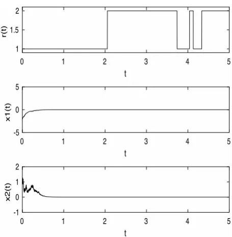
then the discrete-time-state feedback controlled hybrid SDE (5.2) is mean-square exponentially stable. The computer simulation (Fig. 2) supports this result clearly.

0 1 2 3 4 5

t 1

1.5 2

r(t)

0 1 2 3 4 5

t -5

0 5

x1(t)

0 1 2 3 4 5

t -1

0 1 2

x2(t)

Fig. 2.Computer simulation of the paths of r(t), x1(t) andx2(t)

for the controlled hybrid SDE (5.2) withτ= 10−3 using the Euler–Maruyama method with step size10−6_{and initial values}

r(0) = 1,x1(0) =−2andx2(0) = 1.

6. Conclusion

In this paper, we have proved that unstablelinear hybrid SDEs, in the form of (2.1),can be stabilized by a feedback control based on discrete-time state and mode

observations.Moreover, we have generalised the theory to a class of nonlinear systems.

Acknowledgements

The author wold like to thank the reviewers and the editor for their very helpful comments and professional suggestions. The authors would also like to thank the Leverhulme Trust (RF-2015-385), the Royal Society of London (IE131408), and the Ministry of Education (MOE) of China (MS2014DHDX020) for their financial support. In particular, the first author would like to thank the University of Strathclyde for awarding her the PhD studentship.

REFERENCES

1. Mao,X., Stabilization of continuous-time hybrid stochastic differential equations by discrete-time feedback control, Automatics 49(12) (2013), 3677-3681.

2. Basak, G.K., Bisi, A. and Ghosh, M.K., Stability of a random diffusion with linear drift, J. Math.

3. Gao, H., Wang, C. and Wang, L., On H∞

performance analysis for continuous-time stochas-tic systems with polytopic uncertainties,Circuits

Systems Signal Processing24(2005), 415–429.

4. He, H., Ho, D.W.C. and Lam, J., Stochastic sta-bility analysis of fuzzy Hopfield neural networks with time-varying delays, IEEE Trans. Circuits

and Systems II: Express Briefs52 (2005), 251 –

255.

5. Hu, L., Mao, X., Almost sure exponential stabilization of stochastic systems by state-feedback control,Automatica44(2008), 465–471. 6. Ji, Y. and Chizeck, H.J., Controllability, stabi-lizability and continuous-time Markovian jump linear quadratic control, IEEE Trans. Automat.

Control35(1990), 777–788.

7. Mao, X., Stability of Stochastic Differential

Equations with Respect to Semimartingales,

Longman Scientific and Technical, 1991.

8. Mao, X., Exponential Stability of Stochastic

Differential Equations, Marcel Dekker, 1994.

9. Mao X., Stochastic Differential Equations and

Their Applications, 2nd Edition, Chichester:

Horwood Pub., 2007.

10. Mao, X., Stability of stochastic differential equations with Markovian switching, Sto. Proc.

Their Appl.79(1999), 45–67.

11. Mao, X., Exponential stability of stochastic delay interval systems with Markovian switching,IEEE

Trans. Auto. Control47(10)(2002), 1604–1612.

12. Mao, X., Stability and stabilization of stochastic differential delay equations, IET Control Theory

& Applications1(6)(2007), 1551–1566.

13. Mao, X., Matasov, A. and Piunovskiy, A.B., Stochastic differential delay equations with Markovian switching, Bernoulli 6(1) (2000), 73–90.

14. Mao, X., Yin, G. and Yuan, C., Stabilization and destabilization of hybrid systems of stochastic differential equations,Automatica43(2007), 264– 273.

15. Mao, X., Lam, J. and Huang, L., Stabilisation of hybrid stochastic differential equations by delay feedback control, Systems & Control Letters 57 (2008), 927–935.

16. Mao, X., Liu, W., Hu, L., Luo, Q. and Lu, J., Stabilization of Hybrid SDEs by Feedback control based on discrete-time state observations,Systems

and Control Letters73(2014), 88-95.

17. Mao, X. and Yuan, C., Stochastic Differential

Equations with Markovian Switching, Imperial

College Press, 2006.

18. Mariton, M., Jump Linear Systems in Automatic

Control, Marcel Dekker, 1990.

19. Mohammed, S.-E.A., Stochastic Functional

Dif-ferential Equations, Longman Scientific and

Technical, 1986.

20. Niu, Y., Ho, D.W.C. and Lam, J., Robust integral sliding mode control for uncertain stochastic systems with time-varying delay, Automatica 41 (2005), 873–880.

21. Shaikhet, L., Stability of stochastic hereditary systems with Markov switching, Theory of

Stochastic Processes2(18)(1996), 180–184.

22. Shi, P., Mahmoud, M.S., Yi, J. and Ismail, A., Worst case control of uncertain jumping systems with multi-state and input delay information,

Information Sciences176(2006), 186–200.

23. Sun, M., Lam, J., Xu, S. and Zou, Y.,

Robust exponential stabilization for Markovian jump systems with mode-dependent input delay,

Automatica43(2007), 1799–1807.

24. Willsky, A.S. and Levy,B.C., Stochastic stability research for complex power systems, DOE

Contract, LIDS, MIT, Report ET-76-C-01-2295,

1979.

25. Wang, Z., Qiao, H., Burnham, K.J., On stabi-lization of bilinear uncertain time-delay stochastic systems with Markovian jumping parameters,

IEEE Trans. Automat. Control47(4)(2002), 640–

646.

26. Wu, L., Shi, P. and Gao, H., State estimation and sliding mode control of Markovian jump singular systems,IEEE Trans on Automatic Control55(5) (2010), 1213-1219.

27. Wu, L., Su, X. and Shi, P., Sliding mode control with boundedL2gain performance of Markovian jump singular time-delay systems, Automatica

48(8)(2012), 1929–1933.

28. Wei, G., Wang, Z., Shu, H. and Fang, J., Robust H∞ control of stochastic time-delay

jumping systems with nonlinear disturbances,

Optim. Control Appl. Meth.27(2006), 255–271.

29. Xu, S., Lam, J., Wang J.L. and Yang, G.H., Stabilization and H∞ control for uncertain

stochastic time-delay systems via non-fragile controllers, Asian Journal of Control 8 (2006), 197–200.

30. Yue, D. and Han, Q., Delay-dependent exponential stability of stochastic systems with time-varying delay, nonlinearity, and Markovian switching,

IEEE Trans. Automat. Control 50 (2005), 217–

222.

c