A collocation method based on one-dimensional RBF interpolation scheme for solving PDEs

A collocation method based on one-dimensional RBF

interpolation scheme for solving PDEs

N. Mai-Duy

_{and R.I. Tanner}

School of Aerospace, Mechanical and Mechatronic Engineering,

The University of Sydney, NSW 2006, Australia

Submitted to

International Journal of Numerical Methods for Heat &

Fluid Flow

, 27-October-2005; Revised 6-April-2006

Abstract

Purpose – To present a new collocation method for numerically solving partial differential

equations (PDEs) in rectangular domains.

Design/methodology/approach– The proposed method is based on a Cartesian grid and a

one-dimensional integrated-radial-basis-function (1D-IRBF) scheme. The employment of

inte-gration to construct the RBF approximations representing the field variables facilitates a fast

convergence rate, while the use of a 1D interpolation scheme leads to considerable economy in

forming the system matrix and improvement in the condition number of RBF matrices over a

2D interpolation scheme.

Findings – The proposed method is verified by considering several test problems governed by

second- and fourth-order PDEs; very accurate solutions are achieved using relatively coarse

grids.

Research limitations/implications – Only 1D and 2D formulations are presented, but we

believe that extension to 3D problems can be carried out straightforwardly. Further

develop-ment is needed for the case of non-rectangular domains.

Originality/value – The contribution of this paper is a new effective collocation formulation

based on RBFs for solving PDEs.

Keywords: integrated radial basis function, collocation method, Cartesian grid, multiple

boundary conditions.

Paper type: Research paper

1

Introduction

Radial-basis-function networks (RBFNs) have become one of the main fields of research

in numerical analysis (Haykin, 1999). It has been proved that RBFNs have the property

of universal approximation, i.e. an arbitrary continuous function can be approximated to

Sandberg, 1991). Madych and Nelson (1988,1990) showed that the RBF interpolation

scheme using multiquadrics (MQ) can offer exponential convergence rates/spectral

accu-racy. The application of MQ-RBFNs for the numerical solution of differential equations

has received a great deal of attention over the past 15 years (see, for example, Kansa,

1990; Fasshauer, 1997; Zerroukat et al, 1998; Mai-Duy and Tran-Cong, 2001; Fedoseyev

et al, 2002; Power and Barraco, 2002; Cheng et al, 2003; Larsson and Fornberg, 2003;

Sarler et al, 2004). These global methods had considerable success in solving a variety of

scientific and engineering problems governed by differential equations.

However, it should be noted that the resultant RBF matrices are dense and their condition

numbers grow rapidly as the number of nodes is increased. To resolve this problem, several

attempts to use local RBF approximations (e.g Shu et al, 2003; Lee et al, 2003) or to

combine RBF and domain decomposition (e.g Dubal, 1994; Kansa and Hon, 2000; Li and

Hon, 2004) have been made. For a local-approximation based approach, only a small

region associated with a point, a node’s region of influence, is activated to construct

the RBF approximations for that point. The two most common shapes of an influence

domain are circles and rectangles. Using a local procedure, the cost of computation can be

modest; for example, the inversion involved in the construction process is conducted for

a series of smaller matrices rather than for a large matrix. For a domain-decomposition

based approach, the given analysis domain is divided into a finite number of subdomains.

The original problem can be then reformulated for each subdomain, leading to a series

of coupled smaller subproblems. The solution is required to be continuous and smooth

across the subdomain interfaces. This can be achieved either by overlapping regions (e.g

Li and Hon, 2004) or by common data points along the interfaces (e.g Dubal, 1994).

Using local approximations or domain decompositions have the following advantages: (i)

the resultant coefficient matrices are sparse/block-banded and hence their solutions are

more efficient, and (ii) it can help prevent the rapid growth of the condition number of

It should also be noted that the performance of the RBF scheme is strongly affected by the

RBF width. To date, there is a lack of mathematical theory for finding appropriate values

of the RBF width. In practice, the RBF width is chosen either by empirical approaches or

by optimization techniques. The latter are expensive, especially for non-linear problems.

Generally, the RBF scheme is more accurate, but less stable with increasing RBF-width.

Recently, an alternative approach based on integration to construct the RBF expressions

for the interpolation of functions and the solution of differential equations was proposed

(Mai-Duy and Tran-Cong, 2001,2003). It was found that the indirect/integration-based

RBFN approach (IRBFN) outperforms the direct/differentiation-based RBFN approach

(DRBFN) regarding accuracy and convergence rate over a wide range of the RBF width.

The improvement is attributable to the fact that integration is a smoothing operation

and is more numerically stable.

In this study, a collocation method based on a 1D global IRBF interpolation scheme

for the solution of 2D-PDEs is proposed. A rectangular domain of computation is

dis-cretized using a Cartesian grid (For the case of a non-rectangular domain, prior coordinate

transformation can be conducted to produce a rectangular domain in the computational

space). With the use of IRBFNs, one can make the approximating functions smoother,

and generate additional coefficients (integration constants) that can be used to impose

the governing equation on boundaries and/or to incorporate normal derivative boundary

conditions more efficiently. On the other hand, with the use of a 1D global

interpola-tion scheme, the construcinterpola-tion of RBF approximainterpola-tions for a given point x involves only points that lie on lines intersected at x and parallel to x₋ and y₋axes, rather than the whole set of grid points. This improves the conditioning of the system and requires less

computational work than the case of using a higher-dimensional scheme. One important

feature of the present scheme is that it still maintains the advantages of a global

high-order method such as the capability to achieve a high degree of accuracy using relatively

system matrix limits the use of a global 2D-RBF collocation method to a few hundred

interpolation points. With the present approach, much larger numbers of nodes (e.g, up

to 10201 nodes in this study) can be employed. Numerical results show that the proposed

method achieves a high degree of accuracy.

The remainder of the paper is organized as follows. The proposed 1D-IRBF collocation

method for the solution of second- and fourth-order PDEs is presented and verified in

section 2 and 3, respectively. The method is then applied to simulate the

thermally-driven cavity flow in Section 4. Section 5 gives some concluding remarks.

2

Second-order PDEs

2.1

The IRBF formulation

The domain of interest is discretized using a Cartesian grid, i.e. an array of straight lines

that run parallel to the x₋ and y₋axes. Let Nx and Ny be the numbers of grid lines

in the x₋ and y₋directions, respectively. The dependent variable u and its derivatives

are approximated using a 1D-IRBF interpolation scheme. It should be indicated that the

1D interpolation scheme uses onlyNx or Ny nodes (instead of NxNy nodes) to construct

the approximations for a given point, resulting in considerable economy when compared

with an earlier 2D-IRBF interpolation scheme reported in (Mai-Duy and Tran-Cong,

2005). The construction process involves two steps: (i) To use IRBFNs to approximate

the variable u and its derivatives along a straight line, and (ii) To use Kronecker tensor

2.1.1 One-dimensional formulation

Consider a line in a Cartesian grid, e.g the line runs parallel to thex₋axis. The dependent

variable u along this line is sought in the IRBF form. The second-order derivative of

u is decomposed into RBFs; the RBF network is then integrated twice to obtain the

expressions for the first-order derivative of u and the solution u itself

∂2_u(x)

∂x2 =

Nx

X

i=1

w(i)g(i)(x) =

Nx

X

i=1

w(i)H_[2](i)(x), (1) ∂u(x)

∂x =

Nx

X

i=1

w(i)_H(i)

[1](x) +c1, (2)

u(x) =

Nx

X

i=1

w(i)_H(i)

[0](x) +c1x+c2, (3)

where_{w(i)_}Nx

i=1are RBF weights to be determined;{g(i)(x)}

Nx

i=1are known RBFs;H[1](x) = R

H[2](x)dx, H[0](x) = R

H[1](x)dx; and c1 and c2 are integration constants. Here it is

re-ferred to as a second-order 1D-IRBF scheme, denoted by IRBF-2. It is more convenient

to work in physical space than in network-weight space. The RBF coefficients including

two integration constants can be transformed into the meaningful nodal variable values,

based on the following equations

u(x(1)) =

Nx

X

i=1

w(i)_H(i) [0](x

(1)_{) +c}

1x(1)+c2, (4)

u(x(2)) =

Nx

X

i=1

w(i)_H(i) [0](x

(2)_{) +c}

1x(2)+c2, (5)

· · · ·

u(x(Nx)_{) =}

Nx

X

i=1

w(i)H_[0](i)(x(Nx)_{) +c}

The above system can be written in the matrix form

b

u=_H

   wb

b

c

 

, (7)

where_His aNx×(Nx+2) matrix,ub= (u(1), u(2),· · ·, u(Nx))T,wb= (w(1), w(2),· · · , w(Nx))T,

and _bc= (c1, c2)T.

One difference between 1D integrated- and differentiated-RBF interpolation schemes is

that the former possesses a larger set of expansion coefficients owing to the presence of two

integration constants c1 and c2. The present conversion schemes can be thus developed

into two directions.

2.1.2 Non-square conversion matrix (NSCM)

The direct use of (7) leads to an underdetermined system of equations. The associated

matrix is referred to as the conversion matrix, denoted by_C (_C =_H). The pseudo inverse

of _C can be found using the SVD technique. It is noted that the purpose of using SVD

here is to provide a solution whose norm is the smallest in the least-squares sense

b

u=_H

   wb

b

c

  =_C

   wb

bc

 

, (8)

   wb

b

c

 

2.1.3 Square conversion matrix (SCM)

One can add two additional equations of the form

f1 =

Nx

X

i=1

w(i)H_[(_†i_])+c1α1+c2β1, (10)

f2 =

Nx

X

i=1

w(i)H_[(_‡i_])+c1α2+c2β2, (11)

or

b

f =_K

   wb

b

c

 

 (12)

to (7). The conversion system can be written as

   bu

b f   =    H K       wb

b

c

  =_C

   wb

bc

 

. (13)

The conversion matrix _C becomes square, and its inverse can be computed by using the

LU decomposition _

  wb

b

c

  =_C−1

   bu

b

f

 

. (14)

It is widely observed that the RBF approximations have a tendency to produce larger

errors near boundaries. Fedoseyev et al (2002) developed a MQ-RBF collocation method

with PDE collocation on the boundaries; numerical results indicated a considerable

im-provement in accuracy. Motivated by these results, the two extra equations (10) and

(11) can be utilized here to satisfy the governing equation at both ends of the line: x(1)

and x(Nx). If the Neumann boundary condition rather than the Dirichlet condition is

given, these equations can be used to represent normal derivative boundary conditions;

imposition of the governing equation on the boundaries is carried out at a later stage

are known quantities. However, their explicit forms/values depend on the problem to be

solved; they will be presented in some detail in section Numerical Results. A distinct

difference between the differentiation- and integration-based formulations is that the

gov-erning equation is forced to be satisfied exactly on the boundaries by means of fictitious

points inside/outside domain for the former and by integration constants for the latter.

In the following discussion, only the SCM version is considered since the NSCM system

(8) can be obtained from the SCM system (13) by simply setting matrix _K and vector fb to null.

By substituting (14) into (1) and (2), the second- and first-order derivatives of the variable

u will be expressed in terms of nodal variable values

∂2_u(x)

∂x2 =

H_[2](1)(x), H_[2](2)(x),_{· · ·} , H(Nx)

[2] (x),0,0

C−1

   bu

b

f

 

, (15)

∂u(x) ∂x =

H_[1](1)(x), H_[1](2)(x),_{· · ·} , H(Nx)

[1] (x),1,0

C−1    bu

b

f

 

, (16)

or

∂2u(x)

∂x2 =D2xub+k2x, (17)

∂u(x)

∂x =D1xub+k1x, (18)

where k2x and k1x are scalars whose values depend on f1 and f2.

Application of (17) and (18) to every collocation point on the line yields

d

∂2_u

∂x2 =Db2xbu+bk2x, (19) c

∂u

where_Db2x and Db1x are known matrices of dimensionNx×Nx, andbk2x andbk1x are known

vectors of length Nx.

Similarly, along a vertical line, the values of the second- and first-order derivatives of u

with respect to y at the collocation points can be given by

d

∂2_u

∂y2 =Db2ybu+bk2y, (21) c

∂u

∂y =Db1ybu+bk1y. (22)

2.1.4 Two-dimensional formulation

Assuming that the grid points are numbered from bottom to top and from left to right,

one can write the values of the derivatives ofuover the whole domain by using Kronecker

tensor products as follows

g

∂2_u

∂x2 =

b

D2x⊗ Iy

e

u+ek2x =De2xeu+ek2x, (23)

f

∂u ∂x =

b

D1x⊗ Iy

e

u+ek1x =De1xeu+ek1x, (24)

g

∂2_u

∂y2 =

Ix⊗Db2y

e

u+ek2y =De2yeu+ek2y, (25)

f

∂u ∂y =

Ix⊗Db1y

e

u+ek1y =De1yeu+ek1y, (26)

where_Ix andIy are the identity matrices of dimensionNx×Nx andNy×Ny, respectively;

e

k2x, ek1x,ek2y and ek1y are known vectors of lengthNxNy;De2x,De1x, De2y andDe1y are known

matrices of dimensionNxNy ×NxNy; and ue= u(1), u(2),· · ·, u(NxNy)

T

2.2

Numerical results

The accuracy of an approximation scheme is measured by means of the discrete relative

L2 error defined as

Ne =

r PN

i=1

u(ei)−u(i)

2

r PN

i=1

u(ei)

2 , (27)

where N is the number of collocation points; and ue and u are the exact and computed

solutions, respectively. The present study employs multiquadrics (MQ) whose form is

g(i)(x) =

q

kx₋c(i)_k2_+a(i)2_{, (28)}

where c is the centre,a is the RBF width and _k._kdenotes a Euclidean norm. The width of theith MQ-RBF,a(i)_{, is simply chosen to be the minimum distance from theith centre}

to its neighbours.

2.2.1 Problem 1

Consider the following Poisson equation

∇2u=b=₋8π2sin(2πx) sin(2πy). (29)

An approximate solution is sought in the unit square domain, 0 _≤ x, y _≤ 1. The exact

solution is given by

ue = sin(2πx) sin(2πy). (30)

Ten uniform grids, 11_×11, 21_×21, _{· · ·}, 101_×101, are employed. A comparative study

of the accuracy of the present 1D-IRBF method between the two versions, NSCM and

SCM, is carried out for two different types of the boundary condition, namely _{u_} and

Dirichlet boundary condition

Along the two vertical sides, the extra information fi, which are used for computing the

derivatives ofu with respect to x, are taken to be

f1(x= 0, y) =

∂2_u

∂x2(0, y) =b(0, y)−

∂2_u

∂y2(0, y) = 0, (31)

f2(x= 1, y) =

∂2_u

∂x2(1, y) =b(1, y)−

∂2_u

∂y2(1, y) = 0, (32)

or

Nx

X

i=1

w(i)H_[2](i)(0) = 0, (33)

Nx

X

i=1

w(i)H_[2](i)(1) = 0. (34)

Similarly, along the two horizontal sides, the extra information fi, which are used for

computing the derivatives ofu with respect to y, are defined as

f1(x, y = 0) =

∂2_u

∂y2(x,0) =b(x,0)−

∂2_u

∂x2(x,0) = 0, (35)

f2(x, y = 1) =

∂2_u

∂y2(x,1) =b(x,1)−

∂2_u

∂x2(x,1) = 0. (36)

Applying the governing equation (29) at the interior points (ip) yields

e

D2x+De2y

ipeu= (b)ip−

e

k2x

ip−

e

k2y

ip. (37)

Making use of the Dirichlet boundary condition of the problem, a determinate system of

equations is obtained which can be solved by Gaussian elimination.

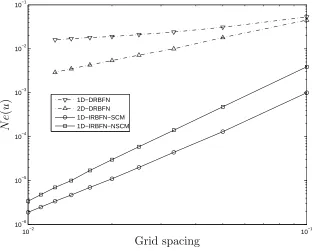
Results concerning the relative L2 error are given in Figure 1 which indicates the rapid

improvement in accuracy with increasing density for both versions. The SCM version is

The present results are also compared with those obtained by the classical DRBFN method

(Figure 1). The DRBFN method that is based on a 1D interpolation scheme is also

implemented here. The 1D- and 2D-DRBF methods use the same network parameters

(e.g the number of collocation points, their locations and the RBF widths) as the proposed

1D-IRBF method. It can be seen that the proposed method outperforms the 1D- and

2D-DRBF methods regarding accuracy and convergence.

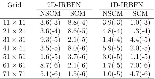
In comparison with the 2D-IRBF method, Table 1 shows that for each version (SCM

and NSCM), the 2D-IRBF method is more accurate than the 1D-IRBF method. It is

interesting to note that the accuracy of the 1D-IRBF method with SCM is superior to that

of the 2D-IRBF method with NSCM. The 2D method requires much more computational

effort than the 1D method. For example, the inversion is conducted for matrices of

dimensions aboutNx×NxorNy×Ny for the 1D method, but of dimensionsNxNy×NxNy

for the 2D method.

Dirichlet and Neumann boundary conditions

The Neumann boundary conditions are imposed on the two vertical sides, while the

Dirich-let conditions are specified along the two horizontal sides. Special attention here is given

to the implementation of the Neumann boundary condition. The two additional equations

(10) and (11) can take the form

f1(x= 0, y) =

∂u

∂x(0, y) = 2πsin(2πy), (38) f2(x= 1, y) =

∂u

or

Nx

X

i=1

w(i)_H(i)

[1](0) +c1 = 2πsin(2πy), (40)

Nx

X

i=1

w(i)_H(i)

[1](1) +c1 = 2πsin(2πy). (41)

For the SCM version, the governing equation (29) is forced to be satisfied not only at the

interior points but also at the 2(Ny −2) boundary points on the two vertical sides. For

the NSCM version, the governing equation (29) is applied at the interior points and the

Neumann boundary conditions are enforced explicitly by adding some additional equations

to the system. After introducing the Dirichlet boundary condition of the problem, for

both versions, a square algebraic system of dimension (NxNy−2Nx)×(NxNy −2Nx) is

obtained for the unknown nodal values of u inside the domain and on the boundaries of

the Neumann boundary condition.

Figure 2 presents the convergence behaviour of the present method using NSCM and SCM.

It is clear that both versions have essentially the same convergence rates, but the latter

produces a higher degree of accuracy. Imposition of the Neumann boundary condition

through the conversion process is recommended for use because of its superior accuracy

and its straightforward implementation.

3

Fourth-order PDEs

One distinct feature of problems governed by fourth-order PDEs is that there are two

required values of the variable at each boundary point. For the conventional

implementa-tion of multiple boundary condiimplementa-tions, fictitious points are introduced outside/inside the

domain (the fictitious-point technique) or the differential equations are collocated at a

is referred to References (e.g Shu, 2000; Shu et al, 2000; Chen et al, 2000) for a more

detailed discussion of this topic. In the present work, the imposition of multiple

bound-ary conditions is simply conducted by means of integration constants; its performance is

compared with that of the node-reduction technique. The details of implementing

mul-tiple boundary conditions using integration constants were reported in (Mai-Duy, 2005;

Mai-Duy and Tanner, 2005).

For the sake of simplicity, the following discussion is given to the case of biharmonic

equations of the form

∂4_u

∂x4 + 2

∂4_u

∂x2_∂y2 +

∂4_u

∂y4 =b(x, y) (42)

in the rectangular domain, subject to the boundary conditions u and ∂u/∂n along the

boundaries.

The process of deriving the 1D-IRBF formulation for fourth-order PDEs is similar to

that for second-order PDEs. However, the corresponding equations involve more terms.

Furthermore, special attention needs to be paid to the treatment of mixed partial

deriva-tives, e.g∂4_u/∂x2_∂y2_{. Notations used in this section and in the previous one have similar}

3.1

The IRBF formulation

3.1.1 One-dimensional formulation

The variable u and its derivatives along a grid line that runs parallel to the x₋axis can

be approximated by

∂4_u(x)

∂x4 =

Nx

X

i=1

w(i)g(i)(x) =

Nx

X

i=1

w(i)H_[4](i)(x), (43) ∂3_u(x)

∂x3 =

Nx

X

i=1

w(i)H_[3](i)(x) +c1, (44)

∂2_u(x)

∂x2 =

Nx

X

i=1

w(i)H_[2](i)(x) +c1x+c2, (45)

∂u(x) ∂x =

Nx

X

i=1

w(i)H_[1](i)(x) +c1

x2

2 +c2x+c3, (46)

u(x) =

Nx

X

i=1

w(i)H_[0](i)(x) +c1

x3

6 +c2 x2

2 +c3x+c4, (47)

in which the fourth-order derivative of the variable u is decomposed into RBFs. Here it

is referred to as a fourth-order 1D-IRBF scheme, denoted by IRBF-4.

Some relevant matrices and vectors to be used for the conversion process are given below

H =         

H_[0](1)(x(1)_{) H}(2)

[0](x(1)) · · · H (Nx)

[0] (x(1)) x(1)3/6 x(1)2/2 x(1) 1

H_[0](1)(x(2)_{) H}(2)

[0](x(2)) · · · H (Nx)

[0] (x(2)) x(2)3/6 x(2)2/2 x(2) 1

· · · ·

H_[0](1)(x(Nx)_{) H}(2)

[0] (x(

Nx)_{) · · · H}(Nx)

[0] (x(

Nx)_{) x}(Nx)3_{/6 x}(Nx)2_{/2 x}(Nx) ₁

         b w=          w(1) w(2) · · ·

w(Nx)

        

, _bc=

         c1 c2 c3 c4         

, u_b=

         u(1) u(2) · · ·

u(Nx)

3.1.2 Non-square conversion matrix (NSCM)

The unknown expansion coefficients can be converted into the nodal variable values

ac-cording to the following relation

b

u=_H

   wb

b

c

  =_C

   wb

bc

 

, (48)

   wb

b

c

  =_C−1

b

u. (49)

3.1.3 Square conversion matrix (SCM)

The presence of four integration constants allows the addition of 4 extra equations to the

conversion system. Using information on the governing equation and normal derivative

boundary conditions at both ends of the line, the additional matrix and vector can be

generated as follows

K=         

H_[1](1)(x(1)_{) H}(2)

[1](x(1)) · · · H (Nx)

[1] (x(1)) x(1)2/2 x(1) 1 0

H_[1](1)(x(Nx)_{) H}(2)

[1] (x(

Nx)_{) · · · H}(Nx)

[1] (x(

Nx)_{) x}(Nx)2_{/2 x}(Nx) _{1 0}

H_[4](1)(x(1)_{) H}(2)

[4](x(1)) · · · H (Nx)

[4] (x(1)) 0 0 0 0

H_[4](1)(x(Nx)) H(2)

[4] (x

(Nx)) · · · H(Nx)

[4] (x

(Nx)) 0 0 0 0

         , b f =          ∂u ∂x(x

(1)₎

∂u ∂x(x

(Nx))

b(x(1)₎₋₂ ∂4_u

∂x2_y2(x(1))−

∂4_u

∂y4(x(1))

b(x(Nx))−2 ∂4u

∂x2_y2(x(

Nx))− ∂4u

∂y4(x(

Nx))

The conversion process thus becomes

   bu

b f   =    H K       wb

b

c

  =_C

   wb

bc

 

, (50)

   wb

b

c

  =_C−1

   bu

b

f

 

. (51)

Substitution of (51) into (43)-(46) yields

∂4_u(x)

∂x4 =

H_[4](1)(x), H_[4](2)(x),_{· · ·} , H(Nx)

[4] (x),0,0,0,0

C−1    ub

b

f

 

, (52)

∂3_u(x)

∂x3 =

H_[3](1)(x), H_[3](2)(x),_{· · ·} , H(Nx)

[3] (x),1,0,0,0

C−1    ub

b

f

 

, (53)

∂2_u(x)

∂x2 =

H_[2](1)(x), H_[2](2)(x),_{· · ·} , H(Nx)

[2] (x), x,1,0,0

C−1

   bu

b

f

 

, (54)

∂u(x) ∂x =

H_[1](1)(x), H_[1](2)(x),_{· · ·} , H(Nx)

[1] (x),

x2

2, x,1,0

C−1    bu

b

f

 

. (55)

The values of the ith-order derivative of u (i = _{1,2,3,4_}) at the grid points along a

horizontal line can be computed by

d

∂i_u

∂xi =Db IV ix

   ub

b

f

 

, i=_{1,2,3,4_}, (56)

where the superscriptIV is used to indicate that_Dbix is obtained using the IRBF-4 scheme;

and_DbIV

ix is a known matrix of dimensionNx×(Nx+4); and∂c

i_u

∂xi =

∂i_u

∂xi

(1)

,∂i_u

∂xi

(2)

,_{· · ·} ,∂i_u

∂xi

(Nx)T

Expression (56) can be rewritten as

d_∂i_u

∂xi =Dc1 IV

ix bu+Dc2 IV

ix f ,b (57)

where _Dc1IVix and Dc2 IV

ix are matrices that are formed by the first Nx columns and the last

four columns of the matrix _DbIV

ix , respectively. Unlike the case of second-order PDEs, the

extra information vector fb(components f3 and f4) contains some unknown values—the

mixed partial derivative ∂4u/∂x2∂y2 at the two boundary points. The treatment is as

follows. These unknown values will be replaced by linear combinations of nodal values of

the variable u (the detailed expression of ∂4_u/∂x2_∂y2 _{will be given in section 3.1.4). In}

the same way, one can obtain the values of the ith-order derivative of u with respect toy

along a vertical line.

3.1.4 Two-dimensional formulation

Making use of the following expression

∂4_u

∂2_x∂2_y =

1 2 ∂2 ∂x2

∂2_u

∂y2 + ∂ 2 ∂y2

∂2_u

∂x2

, (58)

the mixed fourth-order partial derivative can be computed by the 1D IRBF-2 scheme with

the extra information fi being the values of the first-order derivatives at the boundary

points which are given or can be computed easily. Expression (58) can be rewritten as

g

∂4_u

∂x2_∂y2 =

1 2 De2x

g

∂2_u

∂y2 +ek2x+De2y g

∂2_u

∂x2 +ek2y ! , (59) = 1 2 e

D2xDe2y+De2yDe2x

e

u+ek4xy, (60)

where _De2x and De2y are known matrices obtained from (23) and (25); ek4xy is a known

vector of length NxNy; De4xy is a know matrix of dimension NxNy ×NxNy; and g∂

4_u

∂x2_∂y2 =

∂4_u

∂x2_∂y2

(1)

,_∂x∂24_∂yu2

(2)

,_{· · ·} ,_∂x∂24_∂yu2

(NxNy)T

.

It can be seen that the mixed fourth-order partial derivative of the variable u is now

ex-pressed in terms of nodal variable values. Using these results to represent the components

f3 and f4, one can now extend the approximations for ∂iu/∂xi (57) to a 2D domain by

means of Kronecker tensor products. Their final forms can be written as

g

∂i_u

∂xi =De IV ix eu+ek

IV

ix (62)

g

∂i_u

∂yi =De IV iy eu+ek

IV

iy (63)

where i=_{1,2,3,4_};ekIV

ix and ekiyIV are known vectors of length NxNy; and DeixIV and DeiyIV

are known matrices of dimension NxNy ×NxNy.

3.2

Numerical results

A biharmonic Dirichlet problem is considered here to verify the 1D-IRBF formulation.

3.2.1 Problem 2

Consider the biharmonic equation

in the domain 0_≤x, y _≤1, subject to the boundary conditions

u= 0 along the boundaries, ∂u

∂x = 2πsin(2πy) x= 0, x= 1 ∂u

∂y = 2πsin(2πx) y= 0, y = 1

The exact solution is given by

ve(x, y) = sin(2πx) sin(2πy). (65)

A number of uniform grids, 6_×6, 11_×11, ..., and 71_×71, are employed. In forming the

system matrix, the SCM version allows the biharmonic equation (64) to be collocated at

every interior point. For the NSCM version, it is necessary to reduce the number of interior

points used for (64) in order to impose the boundary conditions ∂u/∂n; these interior

points chosen here for collocating the biharmonic equation are (xi, yj) with 3 ≤i≤Nx−2

and 3 _≤ j _≤ Ny −2. A comparison of the accuracy of the present method between the

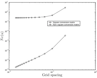
two versions is given in Figure 3. The NSCM version does not perform as well, probably

due to the fact that the governing equation is not forced to be satisfied exactly at every

interior point. For the SCM version, a high degree of accuracy and fast convergence are

achieved.

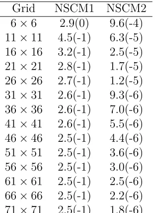
The question here is whether the accuracy of the NSCM approach is improved when one

tries to impose the normal derivative boundary conditions through the conversion process

(NSCM2). In this case, the dimension of conversion matrices is (Nx+ 2)×(Nx+ 4). Table

2 reveals that this implementation leads to a significant improvement in accuracy over

the traditional node-reduction technique.

Numerical results show that both SCM and NSCM versions of the proposed 1D-IRBF

underdeter-mined matrices, while the latter involves the inversion of square matrices. Fortunately,

these calculations are conducted in 1D-domains only, and hence they do not add greatly

to the computational cost. The classical DRBFN method does not require such inversions,

but its approximations involve all data points. It should be emphasized the final matrices

obtained by the IRBFN and DRBFN methods have similar sizes.

For the SCM version, to impose the governing equation on the boundaries, the values of

relevant derivatives at the boundary points should be known or should be written in terms

of nodal variable values. It is difficult to meet this requirement when extending the SCM

version to the case of irregular domains. One possible way to overcome these difficulties is

to apply a technique by Sanmiguel-Rojas et al (2005) to generate a non-uniform Cartesian

grid in which all the boundary nodes are regular nodes of the grid. For the NSCM version,

one does not need to concern these issues when extending it to irregular domains.

4

Natural convection flow in a square slot

The proposed method is applied here to simulate the thermally-driven cavity flow in a

square slot. For this problem, the governing equation presents the coupling of momentum

(fourth-order PDE, streamfunction formulation) and energy (second-order PDE)

equa-tions. Very thin boundary layers are formed at high values of the Rayleigh number,

thereby making the numerical simulation difficult. This problem provides a good means

for testing and validating new numerical methods. From the literature, a range of the

Rayleigh number from 103 _{to 10}6 _{is usually employed for the verification of numerical}

methods. It will be shown that converged solutions for higher-Rayleigh-numbers are

achieved with the present method, and the obtained RBF results are in very good

T and streamfunctionψ behaviour can be written as ∂T ∂t + ∂ψ ∂y ∂T ∂x − ∂ψ ∂x ∂T ∂y

= _√ 1 RaP r

∂2_T

∂x2 +

∂2_T

∂y2

, (66)

− _∂t∂

∂2_ψ

∂x2 +

∂2_ψ

∂y2

+ ∂ψ ∂y

∂3_ψ

∂x3 +

∂2 ∂y2 ∂ψ ∂x

− ∂ψ_∂x

∂2 ∂x2 ∂ψ ∂y + ∂ 3_ψ ∂y3 = − r P r Ra

∂4_ψ

∂x4 +

∂2

∂x2

∂2_ψ

∂y2 + ∂ 2 ∂y2

∂2_ψ

∂x2 +∂ 4_ψ ∂y4 +∂T

∂x, (67)

where Ra and P r are the Rayleigh number and the Prandtl number, respectively. The

variables are normalized here using reference quantities recommended by Ostrach (1988)

for the case of pRa/P r > 1 and P r <1. These non-dimensional equations are written in detail in order to show how their derivative terms are computed, e.g mixed third-order

partial derivatives are determined through relevant second- and first-order derivatives.

A square cavity of a unit size, containing a fluid of P r = 0.71, is considered.

Non-slip boundary conditions (ψ = 0 and ∂ψ/∂n) are imposed along all the walls. The

thermal boundary conditions are T = 0.5 and T = ₋0.5 (isothermal) along the left and

right walls, respectively, and ∂T /∂y = 0 (adiabatic) along the bottom and top walls.

The benchmark solutions for this problem can be found in (de Vahl Davis, 1983) for

103 _{≤ Ra ≤ 10}6 _{and in (Le Quere, 1991) for Ra ≥ 10}6_{. The former used second-order,}

finite-central-difference approximations and a Richardson extrapolation scheme, while the

latter employed a pseudo-spectral Chebyshev algorithm using the spatial resolution up to

a 128_×128 polynomial expansion.

The present solution procedure involves the following steps

1. Guess a set of initial conditions: T, ψ and their spatial derivatives

2. Discretize in time using a first-order accuracy finite-difference scheme, where the

diffusive and convective terms are treated implicitly and explicitly, respectively

3. Discretize in space using 1D-IRBF schemes with NSCM2:

Solve the momentum equation (67) for ψ

4. Check to see whether the solution has reached a steady state

r PN

i=1

ψ(_ki₊₁) ₋ψ_k(i)2

r PN

i=1

ψ_k(i₊₁) 2

< ǫ, (68)

where k is the time level, ǫ is the tolerance and N is the number of collocation

points.

5. If it is not satisfied, advance time step and repeat from step 2. Otherwise, stop the

computation and output the results.

Normal derivative boundary conditions ∂ψ/∂nand ∂T /∂y are imposed by means of

inte-gration constants. The energy equation (second-order PDE) is collocated not only at the

interior points but also at the boundary points on the bottom and top walls.

A range of Ra= _{105_,106_,107_{} is considered here. The computed solution at the lower}

and nearest value of Ra is taken to be the initial solution. Seven uniform grids, namely

21_×21,31_×31,_{· · ·},81_×81, are employed to study the convergence behaviour of the

method. Time steps are chosen to be 0.1 for Ra = 105_{, 0.05 for Ra = 10}6 _{and 0.01 for}

Ra= 107_.

The following quantities are of interest to this type of flow

1. the maximum horizontal velocity umax on the vertical mid-plane of the cavity and

its location

2. the maximum vertical velocity vmax on the horizontal mid-plane of the cavity and

3. the average Nusselt number throughout the cavity

Nu =

Z 1

0

Nu(x)dx (69)

Nu(x) =

Z 1

0

uT ₋ ∂T ∂x

dy (70)

The present velocity components are related to the corresponding benchmark solutions

(de Vahl Davis, 1983) according to the relation

√

RaP r(u, v)present = (u, v)benchmark.

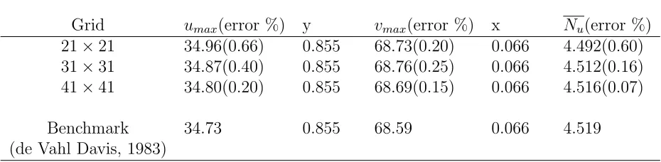
The results obtained are given in Tables 3-5, which show the rapid improvement in

accu-racy as the density increases. Although very sharp gradients are formed at high values

of the Rayleigh number, the present method achieves very accurate results. For example,

the maximum error is less than 0.2% for Ra= 107 _{using a grid of 81×81.}

Figure 4 shows the streamlines, isotherms and iso-vorticity lines of the flow at Ra= 107

using a grid of 81_×81. Every plot contains 17 contour lines whose values vary linearly

from the minimum to maximum values, and they look reasonable when compared to the

benchmark solutions.

5

Concluding remarks

This paper reports a collocation method based on a one-dimensional

integrated-radial-basis-function interpolation scheme for the solution of second- and fourth-order PDEs

in rectangular domains. The use of integrated RBFs allows (i) the normal derivative

boundary condition to be incorporated more efficiently and (ii) the exact satisfaction of

PDEs not only at the interior points but also at the boundary points. The imposition of

for use. On the other hand, the employment of a 1D interpolation scheme instead of 2D

interpolation scheme permits relatively large numbers of data points to be employed. The

present one-dimensional global IRBF scheme is demonstrated on a number of test cases,

including the benchmark natural convection problem; a very high degree of accuracy is

achieved using relatively coarse grids. Extension of the proposed method to the case of

non-rectangular domains is currently underway, and it will be reported in future work.

ACKNOWLEDGEMENTS

N. Mai-Duy wishes to thank the University of Sydney for a Sesquicentennial Post-doctoral

Research Fellowship. We would like to thank the referees for their helpful comments and

suggestions to improve the paper.

REFERENCES

1. Cheng, A.H.-D., Golberg, M.A., Kansa, E.J. and Zammito, G. (2003) “Exponential

convergence and H-c multiquadric collocation method for partial differential

equa-tions”, Numerical Methods for Partial Differential Equations, Vol 19, pp. 571-94.

2. Chen, W., Shu, C., He, W. and Zhong, T. (2000) “The application of special matrix

product to differential quadrature solution of geometrically nonlinear bending of

orthotropic rectangular plates”, Computers & Structures, Vol 74, pp. 65–76.

3. de Vahl Davis, G. (1983) “Natural convection of air in a square cavity: a bench

mark numerical solution”, International Journal for Numerical Methods in Fluids,

Vol 3, pp. 249-64.

4. Dubal, M.R. (1994) “Domain decomposition and local refinement for multiquadric

approximations. I: Second-order equations in one-dimension”, Journal of Applied

Science and Computation, Vol 1 No 1, pp. 146-71.

5. Fasshauer, G.E. (1997), “Solving partial differential equations by collocation with

Surface Fitting and Multiresolution Methods, Vanderbilt University Press, Nashville,

TN, pp. 131-38.

6. Fedoseyev, A.I., Friedman, M.J. and Kansa, E.J. (2002) “Improved multiquadric

method for elliptic partial differential equations via PDE collocation on the

bound-ary”,Computers & Mathematics with Applications, Vol 43 No 3-5, pp. 439-55.

7. Haykin, S. (1999), Neural Networks: A Comprehensive Foundation, Prentice-Hall,

New Jersey.

8. Kansa, E.J. (1990) “Multiquadrics- A scattered data approximation scheme with

applications to computational fluid-dynamics-II. Solutions to parabolic, hyperbolic

and elliptic partial differential equations”,Computers and Mathematics with

Appli-cations, Vol 19 No 8-9, pp. 147-61.

9. Kansa, E.J. and Hon, Y.C. (2000) “Circumventing the ill-conditioning problem with

multiquadric radial basis functions: applications to elliptic partial differential

equa-tions”, Computers and Mathematics with Applications, Vol 39, pp. 123-37.

10. Larsson, E. and Fornberg, B. (2003) “A numerical study of some radial basis

func-tion based solufunc-tion methods for elliptic PDEs”, Computers and Mathematics with

Applications, Vol 46, pp. 891-902.

11. Lee, C.K., Liu, X. and Fan S.C. (2003) “Local multiquadric approximation for

solving boundary value problems”, Computational Mechanics, Vol 30 No 5-6, pp.

396-409.

12. Le Quere, P. (1991) “Accurate solutions to the square thermally driven cavity at

high Rayleigh number”, Computers & Fluids, Vol 20 No 1, pp. 29–41.

13. Li, J. and Hon, Y.C. (2004) “Domain decomposition for radial basis meshless

14. Madych, W.R. and Nelson, S.A. (1988) “Multivariate interpolation and

condition-ally positive definite functions”, Approximation Theory and its Applications, Vol 4,

pp. 77-89.

15. Madych, W.R. and Nelson, S.A. (1990) “Multivariate interpolation and

condition-ally positive definite functions, II”, Mathematics of Computation, Vol 54 No 189,

pp. 211-30.

16. Mai-Duy, N. (2005) “Solving high order ordinary differential equations with radial

basis function networks”,International Journal for Numerical Methods in

Engineer-ing, Vol 62, pp. 824-52.

17. Mai-Duy, N. and Tanner, R.I. (2005) “Solving high order partial differential

equa-tions with radial basis function networks”, International Journal for Numerical

Methods in Engineering, Vol 63, pp. 1636-54.

18. Mai-Duy, N. and Tran-Cong, T. (2001) “Numerical solution of differential equations

using multiquadric radial basis function networks”, Neural Networks, Vol 14 No 2,

pp. 185-99.

19. Mai-Duy, N. and Tran-Cong, T. (2003) “Approximation of function and its

deriva-tives using radial basis function networks”,Applied Mathematical Modelling, Vol 27,

pp. 197-220.

20. Mai-Duy, N. and Tran-Cong, T. (2005) “An efficient indirect RBFN-based method

for numerical solution of PDEs”, Numerical Methods for Partial Differential

Equa-tions, Vol 21, pp. 770-90.

21. Ostrach, S. (1988) “Natural convection in enclosures”, Journal of Heat Transfer,

Vol 110, pp. 1175-90.

22. Park, J. and Sandberg, I.W. (1991) “Universal approximation using radial basis

23. Power, H. and Barraco, V. (2002) “A comparison analysis between unsymmetric

and symmetric radial basis function collocation methods for the numerical solution

of partial differential equations”, Computers and Mathematics with Applications,

Vol 43, pp. 551-83.

24. Sanmiguel-Rojas, E., Ortega-Casanova, J., del Pino, C. and Fernandez-Feria, R.

(2005) “A Cartesian grid finite-difference method for 2D incompressible viscous

flows in irregular geometries” Journal of Computational Physics, Vol 204, pp. 302–

318.

25. Sarler, B., Perko, J. and Chen, C.S. (2004) “Radial basis function collocation method

solution of natural convection in porous media”,International Journal of Numerical

Methods for Heat & Fluid Flow, Vol 14 No 2, pp. 187-212.

26. Shu, C. (2000),Differential Quadrature and Its Application in Engineering.

Springer-Verlag, London.

27. Shu, C., Chen, W. and Du, H. (2000) “Free Vibration Analysis of Curvilinear

Quadrilateral Plates by the Differential Quadrature Method”,Journal of

Computa-tional Physics, Vol 163, pp. 452–466.

28. Shu, C., Ding, H. and Yeo, K.S. (2003) “Local radial basis function-based

differen-tial quadrature method and its application to solve two-dimensional incompressible

Navier-Stokes equations”, Computer Methods in Applied Mechanics and

Engineer-ing, Vol 192, pp. 941-54.

29. Zerroukat, M., Power, H. and Chen, C.S. (1998) “A numerical method for heat

transfer problems using collocation and radial basis functions”, International

Table 1: Second-order PDE, Dirichlet boundary conditions: RelativeL2errors obtained by

the 2D- and 1D-IRBF methods. For each version (SCM and NSCM), the 2D-IRBF method is more accurate than 1D-IRBF method. It is interesting to note that the accuracy of the 1D-IRBF method with SCM is superior to that of the 2D-IRBF method with NSCM. The 2D-IRBF method requires much more computational effort than the 1D-IRBF method. a(₋b) means a_×10−b_.

Table 2: Fourth-order PDE: Relative L2 errors obtained by the NSCM1 and NSCM2

ap-proaches. For NSCM1, the multiple boundary conditions are implemented by the node-reduction technique (collocating the governing equation at a smaller number of interior points), while for NSCM2, normal derivative boundary conditions are imposed by means of integration constants. The latter outperforms the former regarding accuracy and con-vergence rate. a(₋b) meansa_×10−b_.

Table 3: Natural convection, Ra= 105_.

Grid umax(error %) y vmax(error %) x Nu(error %)

21_×21 34.96(0.66) 0.855 68.73(0.20) 0.066 4.492(0.60) 31_×31 34.87(0.40) 0.855 68.76(0.25) 0.066 4.512(0.16) 41_×41 34.80(0.20) 0.855 68.69(0.15) 0.066 4.516(0.07)

Table 4: Natural convection, Ra= 106_{. It is noted that the percentage errors presented}

here are relative to the spectral results of Le Quere (1991).

Grid umax(error %) y vmax(error %) x Nu(error %)

51_×51 65.04(0.32) 0.850 220.96(0.16) 0.038 8.816(0.10) 61_×61 64.98(0.23) 0.850 220.83(0.10) 0.038 8.819(0.07) 71_×71 64.94(0.17) 0.850 220.74(0.06) 0.038 8.820(0.06) 81_×81 64.91(0.12) 0.850 220.69(0.04) 0.038 8.821(0.05)

Benchmark 64.63 0.850 219.36 0.038 8.800 (de Vahl Davis, 1983)

Table 5: Natural convection, Ra= 107_.

Grid umax(error %) y vmax(error %) x Nu(error %)

51_×51 143.9(3.16) 0.885 680.8(2.63) 0.021 16.126(2.40) 61_×61 146.9(1.14) 0.881 693.1(0.87) 0.021 16.370(0.93) 71_×71 148.2(0.27) 0.879 698.0(0.17) 0.021 16.463(0.36) 81_×81 148.8(0.13) 0.878 699.7(0.07) 0.021 16.499(0.15)

10−2 10−1

10−6

10−5

10−4

10−3

10−2

10−1

1D−DRBFN 2D−DRBFN 1D−IRBFN−SCM 1D−IRBFN−NSCM

Grid spacing

N

e

(

u

)

Figure 1: Second-order PDE, Dirichlet boundary conditions: Relative L2 errors obtained

10−2 10−1

10−5

10−4

10−3

10−2

10−1

Square conversion matrix Non−square conversion matrix

Grid spacing

N

e

(

u

)

10−2 10−1 100

10−6

10−5

10−4

10−3

10−2

10−1

100

101

Square conversion matrix Non−square conversion matrix

Grid spacing

N

e

(

u

)

Streamlines

Iso-vorticity lines