White Rose Research Online URL for this paper:
http://eprints.whiterose.ac.uk/107576/
Version: Accepted Version
Article:
Campbell, E. and O'Gorman, J. (2016) An efficient magic state approach to small angle
rotations. Quantum Science & Technology, 1. 015007. ISSN 2058-9565
https://doi.org/10.1088/2058-9565/1/1/015007
[email protected] https://eprints.whiterose.ac.uk/ Reuse
Unless indicated otherwise, fulltext items are protected by copyright with all rights reserved. The copyright exception in section 29 of the Copyright, Designs and Patents Act 1988 allows the making of a single copy solely for the purpose of non-commercial research or private study within the limits of fair dealing. The publisher or other rights-holder may allow further reproduction and re-use of this version - refer to the White Rose Research Online record for this item. Where records identify the publisher as the copyright holder, users can verify any specific terms of use on the publisher’s website.
Takedown
If you consider content in White Rose Research Online to be in breach of UK law, please notify us by
Earl T. Campbell1 and Joe O’Gorman2
1
Department of Physics & Astronomy, University of Sheffield, Sheffield, S3 7RH, United Kingdom.∗ 2
Department of Materials, University of Oxford, Oxford, OX1 3PH, United Kingdom.
Standard error correction techniques only provide a quantum memory and need extra gadgets to perform computation. Central to quantum algorithms are small angle rotations, which can be fault-tolerantly implemented given a supply of an unconventional species of magic state. We present a low-cost distillation routine for preparing these small angle magic states. Our protocol builds on the work of Duclos-Cianci and Poulin [Phys. Rev. A 91, 042315 (2015)] by compressing their circuit. Additionally, we present a method of diluting magic states that reduces costs associated with very small angle rotations. We quantify performance by the expected number of noisy magic states consumed per rotation, and compare with other protocols. For modest size angles, our protocols offer a factor 24 improvement over the best known gate synthesis protocols and a factor 2 over the Duclos-Cianci and Poulin protocol. For very small angle rotations, the dilution protocol dramatically reduces costs, giving several orders magnitude improvement over competitors. There also exists an intermediary regime of small, but not very small, angles where our approach gives a marginal improvement over gate synthesis. We discuss how different performance metrics may alter these conclusions.
I. INTRODUCTION
Fault-tolerant quantum computing involves a host of resource overheads, entering at different stages of the pro-cess. The most widely known cost is that of encoding a logical qubit into many physical qubits, which provides safe storage of quantum information. However, once en-coded, a logical qubit only natively supports a limited set of fault-tolerant operations [1]. For high-threshold codes, the native operations belong within the Clifford group. Additional layers of gadgets are required to en-able general purpose quantum computation. A corol-lary of the Solovay-Kitaev theorem [2] is that if the Clif-ford group is augmented by a non-ClifClif-ford T gate, also called the π/8 gate, the device can efficiently approxi-mate any required quantum algorithm. These T gates can in turn be fault-tolerantly performed by using state injection of high-fidelity magic states, prepared by distil-lation [3]. However, the Solovay-Kitaev theorem requires a huge number of T gates, and early magic state distil-lation protocols put a high price on each one. The last decade has seen substantial advances in both these ar-eas. Magic state distillation is now possible at better rates [3–7], reducing the expected cost per high quality T-gate. The number ofT-gates needed to approximate some unitary, the so-calledT-count, has also been signif-icantly reduced after the discovery of new gate synthesis techniques [8–12].
Nevertheless, fault-tolerant quantum computing re-mains a monumental challenge, so further resources sav-ings are essential. One suggested route is to circumvent magic states altogether, for instance by using gauge-fixing [13, 14] of subsystem codes like the 3D colour code [15, 16]. However, this route still pays a price for
|Mℓ • Y
Y Rℓ−1
Rℓ
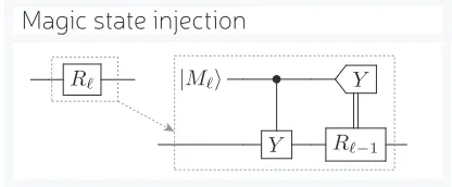
[image:2.612.335.543.286.372.2]Magic state injection
FIG. 1. State-injection using a magic state|Mℓ⟩ to perform
a non-Clifford gateRℓ. If theY-basis measurement outcome
is “+1”, then a correctionRℓ−1 is needed.
gate-synthesis and the additional qubit cost of 3D codes leads to a cubic scaling of overheads that is also achiev-able using magic states [17, 18]. Furthermore, all current indications are that colour codes have a much lower error correction threshold [19] than the toric code [17, 20–22]. For now, such low-noise levels appear beyond technolog-ical reach, ruling out gauge-fixing in the near-term. Al-ternatively, one could work with qudits,d-level systems, which are favourable in terms of the cost of magic state distillation [23–26], though in the qudit context little is known about gate synthesis or experimental feasibility.
Landahl and Cesare [27] were the first to suggest that the gate synthesis overhead could be reduced by distilling different species of magic states, which provide smaller angle rotations instead ofT-gates. Specifically, they con-sidered exp(iπZ/2ℓ) gates for integerℓ, whereℓ= 3 gives theT-gate. These gates are part of an important fam-ily called the Clifford hierarchy [28], with exp(iπZ/2ℓ) residing in the ℓth level of the hierarchy and naturally
vanish.
Progress in gate synthesis has significantly eroded the importance of the Landahl and Cesare result, though their general idea endures. Several researchers found ef-ficient protocols that distill Toffoli magic states [34–36]. Duclos-Cianci and Poulin [37] modified a protocol pro-posed by Meier, Eastin and Knill [4] to prepare magic states that again provide small angle rotations. This re-cent result was a substantial leap forward in the art of distilling magic states for small angle rotations, making magic state distillation cheaper than gate synthesis in many instances. We revisit the work of Duclos-Cianci and Poulin, and find their protocol can be further re-fined. Our proposed alternative requires fewer resources per attempt, and achieves superior error suppression with a higher success probability. Both our protocol and that of Duclos-Cianci and Poulin build on the earlier work of Meier, Eastin, and Knill (MEK) [4].
For very small angle rotations, the required magic states become close to stabiliser states. Duclos-Cianci and Poulin observed that in this regime some magic states in the protocol can be supplanted by stabiliser states, reducing resource costs in a certain regime. In-stead, we introduce the notion of magic state dilution, which takes magic states for ℓ level rotations, and con-verts them into a larger number of magic states for a finer rotations with higherℓ. Error rates are adjusted in the dilution process, and we find it works best at highℓ. Remarkably, dilution can even reduce noise when used at sufficiently highℓ.
II. MAGIC STATES MODEL
First we review the Clifford hierarchy and the magic state model. The well known Pauli groupP is the group composed of tensor products of the single qubit Pauli operators. Unitaries mapping the Pauli group to itself are called Clifford unitaries, which again form a group
C := {U|U P U† ∈ P,∀P ∈ P}. Clifford operations
are physical operations composable from Clifford uni-taries, measurement of Pauli operators and preparation of their eigenstates (the stabiliser states), and classical feedforward. The magic state model of quantum compu-tation [3] assumes Clifford operations are free resources that can be implemented perfectly, and proceeds to eval-uate the cost of non-Clifford operations. Such a model is suitable for logical qubits where the Clifford operations are fault-tolerantly protected, as is common. In our con-clusions, we discuss further the validity of counting only non-Clifford resources.
Unitaries outside the Clifford group can fall into other levels of the Clifford hierarchy, defined recursively as
Cℓ:={U|U P U† ∈ P,∀P ∈ Cℓ−1}, (1)
where C1:=P. It follows that the Clifford group is the
second level, and all higher levels include non-Clifford
gates. We will soon see the Clifford hierarchy plays an im-portant operational role in a teleportation process known as state injection [38].
We introduced small angle rotations in the Z basis, but here it is more convenient to work in the Y basis. We define unitaries Rℓ := exp(iθℓY) with θℓ = π/2ℓ. TheR1 and R2 gates are Clifford, which are presumed
ideal and an inexpensive resource. TheR3 gate is
non-Clifford and equivalent to the T gate. For ℓ ≥ 3, the gates are non-Clifford and belong to theℓth level of the
Clifford hierarchy. Also important here are certain Her-mitian operators in the Clifford hierarchy, and we define Hℓ:=RℓXR†ℓ=R2ℓX =Rℓ−1X and findHℓ∈ Cℓ−1. We
remark thatH3 equals the Hadamard.
Preparation of stabiliser states is also a non-Clifford operation, and these magic states also fall into a natural hierarchy. Recall that stabiliser states are eigen-states of Pauli operators, which are elements ofC1. For
example, the computational basis sates |0⟩ and |1⟩ are stabilised by the Z and −Z Pauli operators, respec-tively. Below we will also make use of the stabiliser states
|±⟩= (|0⟩ ± |1⟩)/√2, which satisfy (±X)|±⟩= |±⟩for PauliX. We consider magic states that are eigenstates of theHℓoperators, so that
|Mℓ⟩=Hℓ|Mℓ⟩=Rℓ|+⟩, (2)
|M¯ℓ⟩= (−Hℓ)|M¯ℓ⟩=Rℓ|−⟩, (3)
which we refer to as ℓth level magic state states. Such
resources can be used to injectRℓrotations into circuits as shown in Fig. (1). The injection procedure is proba-bilistic, and with probability 1/2 it performsRℓand with probability 1/2 it performs R†ℓ. In the latter case a cor-rection ofR2
ℓ =Rℓ−1 is needed to get the desired result.
Since R2 is Clifford, the injection process is ensured to
terminate withinℓ−2 attempts.
Therefore, one can accomplish small angle rotations with a cost that depends on the cost of distilling high-fidelity|Mℓ⟩states. In contrast, gate synthesis methods prescribe distilling just |M3⟩ states and finding a gate
sequence Rℓ ≈C1T C2. . . T Cn in terms of T gates and CliffordsCj. Although, |Mℓ⟩ states will prove more ex-pensive than|M3⟩, gate synthesis can require very many
|M3⟩states, making it more expensive overall. There are
E H
E† H
H
H
=
× •
× • ×
×
• •
× ×
× H ×
=
•
Hℓ
Hℓ Hℓ
• •
E H
E† E
H
E†
H H
H H
H Hℓ H
=
•
Hℓ
Hℓ Hℓ
a b c
ℓ
|+ • • |+
|0
E
R3 R†3
E†
R3 R†3
E†
|0
|0 R3 R†3 R3 R†3 |0
R3 R†3 R3 R†3
R3 R†3 Rℓ−1 X R3 R†3
E
d e
|+ • • |+
|0
E R2
E† E
R2
E†
|0
|0 |0
R3 R†
3 R3 R†3
R3 R†3 Rℓ−1 X R3 R†3
DPℓ
MEKℓ
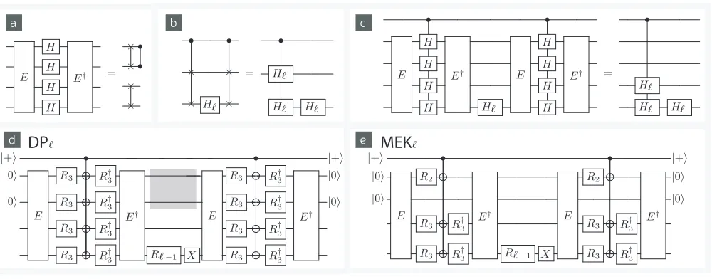
FIG. 2. (a,b,c) Circuit identities and gadgets used to construct distillation protocols. (d) a non-compressed distillation circuit. Adding |0⟩⟨0| measurements and preparations within the grey box gives the DPℓ protocol. (e) the compressed distillation
circuit describing MEKℓ. In both (d) and (e) noisy|Mℓ⟩states are input on the bottom two circuits lines (labelled qubits 3
and 4 in the main text) and allRℓgates withℓ≥3 are approximately implemented by injection of a noisy|Mℓ⟩states.
III. OVERVIEW OF RESOURCE COSTS
Next we summarise the work of Meier, Eastin, and Knill (MEK) [4], upon which Duclos-Cianci and Poulin built their construction. The MEK protocol takes 10 input magic states and with some probability outputs 2 magic states. Therefore, MEK is said to be a 10 →
2 protocol. Accounting for the species of magic states, we call MEK a 103 → 23 protocol where the subscripts
indicate that MEK both inputs and outputs 3rd level magic states. We use DPℓ to label the Duclos-Cianci and Poulin protocol for distilling ℓth level magic states.
Each round of DPℓconsumes a cocktail of different input magic states, and we describe it as a
{
163,2ℓ,1ℓ−1,
(1
2
)
ℓ−2
,
(1
4
)
ℓ−3
, . . .
( 1
2ℓ−3
)
3
}
→2ℓ
(4) protocol. Again, subscripts show what level magic state is used. We show the expected number of inputs re-quired per attempt, which is sometimes a fraction. The fractional sequence terminates at the third level, because lower levels correspond to Clifford resources and are con-sidered free. The DPℓ protocol is presented as a direct generalisation of MEK, but one sees that in the case of ℓ= 3 the DP3protocol is a 183→23protocol and so
ac-tually needs almost twice as many input states as MEK. Here we construct a streamlined variant of DPℓ, that we call MEKℓ and is a
{
83,2ℓ,1ℓ−1,
(
1 2ℓ−2
)
,
(
1 4
)
ℓ−3
, . . .
(
1 2ℓ−3
)
3
}
→2ℓ
(5)
protocol. We find that MEK3 corresponds precisely to
the original MEK, so that MEKℓ is a more apt gener-alisation than DPℓ. Not only does MEKℓ require fewer input resources, it also achieves superior error suppres-sion with a higher success probability.
Both MEK and DPℓmake use of a simple 4 qubit code. We useE, short for encoder, to denote the Clifford circuit that brings qubits into the codespace and acts on pairs of Pauli operators as
(Z1, X1)→(Z1Z2Z3Z4, X1X3X4), (6)
(Z2, X2)→(X1X2X3X4, Z2), (7)
(Z3, X3)→(Z1Z4, X1X3), (8)
(Z4, X4)→(X1X4, Z1Z3). (9)
For Pauli operators, we always use the subscript to de-note which qubit the operator acts upon. Preparing the first two qubits in the state |0⟩ and running the en-coder will yield the code stabilised by Z1Z2Z3Z4 and
X1X2X3X4. The logical state in the codespace is
deter-mined by the initial states of the last two qubits. Having defined the codespace, we now turn to describing DPℓ in more detail, where we will also discuss the important features of the 4-qubit code.
IV. UNCOMPRESSED DPℓPROTOCOL
The protocol DPℓ is illustrated in Fig. (2d). Through-out, we label the top wire as the control qubitc, and the subsequent qubits are labelled 1 to 4. We summarise the main steps of the protocol here
1. Prepare qubitsc, 1 and 2, in stabiliser states|+⟩,
[image:4.612.61.561.51.247.2]a
d
|+ • • |+
|0
E
R3 R†3
E† E
R3 R†3
E†
|0
|0 R3 R†3 R3 R†3 |0
R3 R†3 R3 R†3
R3 R†3 Rℓ−1 X R3 R†3
|+ • • |+
|0
E
R3 R†3
V
R3 R†3
E†
|0
|0 |0
R3 R†3 R3 R†3
R3 R†3 R3 R†3
|+ • • |+
|0
E R3
V
R2 R†3
E†
|0
|0 |0
R3 R†3 R3 R†3
R3 R†3 R3 R†3 e
f |+ • • • • |+
|0
E
R3
V
R2 R†3
E†
|0
|0 |0
R3 R3† R3 R†3
R3 R3† R3 R†3
Q V
•
V R†
3 R3
•
V
=
bV R3
=
R†3
V R2 c
R3 R†3
Q
R2
Q g
=
R†3
[image:5.612.60.558.63.340.2]R3
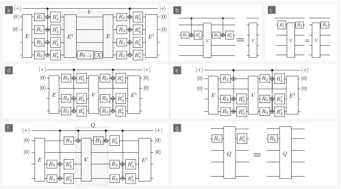
FIG. 3. Circuit identities and reductions used to obtain MEKℓ. (a) circuit before compression, with subcircuitV labelled. (b)
and (c) show properties ofV. (d) shows partially compressed circuit after applying identity (b). (e) further compressed circuit after applying identity (c). In (f) we identify subcircuitQ, with (g) showing a property ofQ. Applying (g) to (f) yields the final compressed circuit, shown in Fig. (2e).
2. Prepare qubits 3 and 4 in noisy|Mℓ⟩states withϵℓ error;
3. Perform the circuit gates shown in Fig. (2d): the R3gates are achieved by state injection using eight
|M3⟩states, andRℓ−1 is achieved with state
injec-tion resulting in overallηℓ−1error;
4. Qubitc is measured inX basis, and we continue if the outcome is “ + 1” and otherwise declare FAIL-URE;
5. Qubits 1 and 2 are measured in Z basis, and we declare SUCCESS if the outcome is “ + 1” and oth-erwise declare FAILURE;
6. If successful, qubits 3 and 4 are output as |Mℓ⟩ states of higher fidelity.
Note that step 3 can include some additional postselected measurements highlighted in Fig. (2d). If included these measurements detect some additional errors, but even without these measurements the protocol quadratically suppresses noise. For simplicity we will assume they are not performed. We next review some of the basic intu-ition behind why DPℓ works, which is closely related to properties of the 4 qubit code used.
The codespace provides both important transversality features and keeps the protocol protected against cer-tain faults. Regarding transversality, a global Hadamard H⊗H⊗H⊗H will preserve the code space, implement-ing a logical SWAP between the two encoded logical bits. More generally, one can verify thatE(H⊗H⊗H⊗H)E†
acts as shown in Fig. (2a). We see that even without fix-ing the first two qubits to|0⟩, this circuit implements a swap and a phase-swap (a swap combined with a phase gate). Furthermore, implementing controlled Hadamards within the encoding will realise controlled versions of the swap and phase-swap. Next, we note that for any Her-mitian unitary, such as Hℓ, we have that conjugation by controlled-swaps will produce a controlledHℓ⊗Hℓas shown in Fig. (2b). We combine this observation with the transversality properties of the code to get the identity of Fig. (2c). An ancilla on the control of the controlled Hℓ⊗Hℓ is used to measure theHℓ⊗Hℓ observable. If the desired magic state is an eigenstate ofHℓ, then mea-suringHℓ⊗Hℓallows us to detect a single error between two noisy |Mℓ⟩ states input on the bottom two circuit lines. In this sense, the codespace has provided a SWAP gadget for distilling noisy|Mℓ⟩magic states.
used to implement these operations. To see this recall thatH =R3XR†3, and so a control-Hadamard can be
im-plemented by a control-X gate sandwiched between R3
andR†3. In turn,R3andR†3can each be implemented at
the cost of a single |M3⟩magic state. Given noisy|M3⟩
magic states, we implement noisyR3 gates. This brings
us to the second role played by the error-correction code. The R3 gates are performed on qubits within an error
correction code that can detect a single qubit error, and so we will detect a single error in any|M3⟩magic states.
Let us explain this point in more detail. When using state injection, if a magic state carries an error, then it will result in Y ·R3 instead of R3, and so there is an
additionalY acting on one of the four qubits. Inside the encoding, the state is an eigenstate of X⊗X⊗X⊗X, but a Y error will cause the state to become an eigen-state of −X ⊗X ⊗X ⊗X. At the end of the circuit, we decode and measure, which is equivalent to measur-ing theX⊗X⊗X⊗X observable. Since we postselect on all +1 outcomes, any error on a single |M3⟩ will be
detected. In contrast, the central Rℓ−1 rotation occurs
outside the protection of the codespace when the logical qubits have been decoded onto single qubits. Therefore, the protocol will not be robust against failure of this gate, and so this rotation must be high fidelity and we herein call it the pivotal rotation. Nevertheless, we can con-struct good distillation protocols provided magic states used in the pivotal rotation have already been distilled to a much higher fidelity than all other elements of the circuit. These high fidelity resources will be costly, but the protocol remains efficient because resources for per-forming Rℓ−1 are less valuable than the |Mℓ⟩ states we are distilling. We are erecting a pyramid of distillation protocols, with resources from lower in the Clifford hier-archy fuelling distillation at higher levels.
V. COMPRESSED MEKℓ PROTOCOL
Our main contribution is to show that this circuit can be compressed into Fig. (2e). This cancels severalR3
ro-tations to reduce the number of magic states consumed. The steps of the protocol roughly follows those numer-ically listed in the previous section, except step 3 now uses the circuit of Fig. (2e), and we use only 8 magic states to inject the R3 gates. It is important that the
circuit retains its fault-tolerance properties through the compression process. That is, even when compressed the noisyR3gates still occur within the four-qubit error
cor-rection code, and so we still expect to detect the failure of any singleR3 gate. In App. B, we present a full noise
analysis that rigorously confirms this intuition.
Here we show how to compress the distillation proto-col, removing unnecessary non-Clifford gates. We start with the protocol shown in Fig. (2d) and through a series of circuit reductions arrive at Fig. (2e). Tak-ing Fig. (2d), we identify a subcircuit V shown in Fig. (3a) inside a shaded box. Next we establish two
properties of V, which are illustrated in Figs. (3b) and (3c). Algebraically, the V circuit is simply V = Eexp(iθℓ−1Y4)X4E†, and using Eqs. (6) we see thatV =
exp(−iθℓ−1Y1Z3X4)Z1Z3. This acts trivially on the
sec-ond qubit and control qubit, entailing the circuit identity of Fig. (3b). Going further, we notice thatV Y1=−Y1V
and so exp(iθ3Y1)V exp(−iθ3Y1) = exp(i2θ3Y1)V.
Us-ing 2θ3 = θ2, we conclude exp(iθ3Y1)Vexp(−iθ3Y1) =
exp(iθ2Y1)V. Recall that exp(iθ2Y1) is the R2 gate
act-ing on qubit 1, and so we have the identity shown in Fig. (3c).
Applying the identity Fig. (3b), shows that Fig. (3d) is equivalent to the original circuit. This observation has eliminated 4 non-Clifford gates. Next, we apply the iden-tity of Fig. (3c), to obtain Fig. (3e). SinceR2is Clifford,
we have removed 2 further non-Cliffords from the circuit. Next, we group together a new collection of circuit ele-mentsQshown in dashed box of Fig. (3f). Algebraically, Qis
Q=Cc,X1exp(iθ2Y1)V Cc,X1 (10)
=Cc,X1exp(iθ2Y1) exp(−iθℓ−1Y1Z3X4)Z1Z3Cc,X1
= exp(iθ2ZcY1) exp(−iθℓ−1ZcY1Z3X4)ZcZ1Z3
where we have used CX for control-X gates and their conjugation relations CX
c,1XcCc,X1 = XcX1 and
CX
c,1Z1Cc,X1 = ZcZ1. From this expression for Q
we can again see that QY1 = −Y1Q, which
en-tails that exp(−iθ3Y1)Qexp(iθ3Y1) = Qexp(i2θ3Y1) =
Qexp(iθ2Y1). This demonstrates the identity of
Fig. (3g). Applying this identity to Fig. (3f), yields the final representation of MEKℓ as shown in Fig. (2e).
VI. MEASURING PERFORMANCE
This section introduces several definitions and nota-tions used to describe the performance of protocols, and quantify their cost.
A. Quantifying noise
Ifρis a noisy|ψ⟩state then we say it has error rateϵ whereϵ:=1
2||ρ− |ψ⟩⟨ψ|||1 and||X||1= tr[
√
XX†] is the
Schatten 1-norm. Unless otherwise stated, we assume diagonal noise so thatρis diagonal in the same basis as
|ψ⟩, and for such states one can show ϵ = 1− ⟨ψ|ρ|ψ⟩. The protocols considered here use a cocktail of input re-sources. We useϵℓ andϵ3to denote the input error rates
of the noisy|Mℓ⟩and|M3⟩states used.
LetU be any rotation of the formU = exp(iθY) andU
be the associated ideal channel. We consider this channel withY noise
E(ρ) = (1−η)U ρU†+ηY U ρU†Y†, (11)
distance measure on channels thend(U,E) =d(1l,U−1◦E)
where 1l is the identity channel. The composite channel
U−1◦ E is a simple Pauli noise channel
(U−1◦ E)(ρ) = (1−η)ρ+ηY ρY†. (12)
A widely used distance measure is derived from the di-amond norm [2], so that d⋄(U,E) := 12||U − E||⋄, and
for Pauli noise of the above type it is well-known that d⋄(U,E) =η.
The diamond norm distance of channels is closely re-lated to the 1-norm distance on states. If a noisy magic state with ϵ error (as measured by 1-norm distance) is used to inject a rotation, then the resulting noisy rota-tion will have error not exceedingϵ(as measured by the diamond norm). Furthermore, diagonal noise on states results in diagonal noise on the rotation. Primarily, we investigate this diagonal noise, but in App. B show that generic noise is also suppressed by MEKℓ.
B. Distillation cost
The output error from MEKℓ is always measured as the error on a single output qubit (ignoring correlations) and we find
δℓ(ϵ3, ϵℓ, ηℓ−1)∼8ϵ23+ϵ2ℓ+ 1
4ηℓ−1+. . . , (13) Psuc(ϵ3, ϵℓ, ηℓ−1)∼1−8ϵ3−2ϵℓ−
1
2ηℓ−1+. . . . (14)
In App. F, we provide the full expressions as calculated by explicit simulation. For η = 0 and ϵ3 = ϵℓ, these expressions are the same as those found by Meier, Eastin and Knill in their analysis of MEK.
Within the context of a single distillation round the performance is independent of the level ℓ, and is solely a function of the noise of the input states ϵℓ, ϵ3 and η.
When we ask how much the input states cost, we find this can increase withℓ. Next, we consider many distillation rounds and combine all performance metrics into a single quantity, the expected resource costC(Mℓ, δ) to distill a
|Mℓ⟩state ofδerror. Lowerδcan require more rounds of distillation, which drives up costs. For our protocol we use that the cost is
C(Mℓ, δℓ) =2C(Mℓ, ϵℓ) + 8C(M3, ϵ3) +C(Rℓ−1, ηℓ−1) 2Psuc(ϵ3, ϵℓ, ηℓ−1)
,
(15) where δℓ obeys Eqs. (13) and (F1). In our analysis, we optimise the cost over many thousands of possible com-binations of input resources by brute force search. No-tice that we capture the cost of the pivotal rotation as C(Rℓ, ηℓ), which will in turn depend on the cost of magic states used to implement the rotation as
C(Rℓ, ηℓ) =C(Mℓ, ϵℓ) +1
2C(Rℓ−1, ηℓ−1), (16)
where
ηℓ= 1 2ϵℓ+
1
2(ϵℓ(1−ηℓ−1) + (1−ϵℓ)ηℓ−1). (17) For the lowest non-Clifford levels, C(M3, δ3) are found by minimising over different combinations of protocols including Bravyi-Haah [5], MEK3 [4] and using the 15
qubit Reed-Muller code [3]. Recall Clifford operations are considered free and perfect so thatC(M2,0) = 0 and C(R2,0) = 0. Throughout we assume that raw initial non-Clifford states can be prepared with a fidelity that is independent of ℓ, and these have unit cost, so that C(Mℓ, ϵraw) = 1. This last assumption is warranted in light of the results of Li [41].
C. Gate-synthesis cost
In general, gate synthesis techniques have an inherent cost that we denote asT(U, ϵGS), whereϵGSis the preci-sion of the synthesis. ThisT-count assumes perfect|M3⟩
magic states are available. Also accounting for the cost of distilled|M3⟩states, the full cost is
CGS(Rℓ, ηℓ) =T(Rℓ, ϵGS)·C(M3, ϵ3) (18) where
ηℓ≃ϵGS+T(Rℓ, ϵGS)·ϵ3. (19)
Notice that gate synthesis has an inherent errorϵGSand
will also fail if one of theTnoisy states fail. In our analy-sis, we present data points for combinations of actual in-stances of gate synthesis using the SR protocol. The SR data is obtained using the Gridsynth package [42]. While SR is optimal for unitary synthesis, lower overheads can be using PQF, which uses ancilla, measurements and feed forward. For PQF, we use the approximation
TP QF(U, ϵGS)≃log
2(
√
2ϵ−1GS) (20)
+ 4 log2(log2(
√
2ϵ−1GS) + 1.187, which is the lowest currently known overhead for gate synthesis. We show in App. B that the notion ofϵused in the gate synthesis literature is comparable to our def-inition.
VII. RESULTS FOR SMALLℓ
We postpone the technical details on noise analysis un-til App. C, and here present results demonstrating the benefits of MEKℓ.
A. Comparison with DP protocol
5 10 15 20 500
1000 1500 2000
5 10 15 20 500
1000 1500 2000 2500 3000
5 10 15 20 1000
2000 3000 4000
5 10 15 20 1000
2000 3000 4000 5000
ℓ=4
5 10 15
fa
ilur
e pr
ob (%)
initial error(%) ǫ
a
0.2 0.4 0.6 0.8 1
Single round performance b Multi-round cost analysis
ℓ=5
ℓ=7
ℓ=6
C
(
H
ℓ
,η
)
Co
st
C
(
H
ℓ
,η
)
Co
st
C
(
H
ℓ
=
,η
)
Co
st
C
(
H
ℓ
,η
)
Co
st
0.2 0.4 0.6 0.8 1 0.05
0.10
initial error (%)ǫ
0.15
err
or out (%)
δ
log10(δ) log10(δ)
[image:8.612.97.519.52.253.2]log10(δ) log10(δ)
FIG. 4. Comparison of the resource cost of distillation using MEKℓand DPℓ. (a) shows performance whenϵ3 =ϵ,ϵℓ=ϵand δ=ϵ2
. These are benchmarked against the standard MEK3 protocol (pink), where the curves for MEKℓ(purple and dotted)
are barely distinguishable from MEK3, whereas DPℓ (blue) performs much worse. The curves for DPℓ are based on leading
order approximations [43]. (b) shows the full resource cost of MEKℓprotocol (purple) and DPℓ(blue) of distilling a|Mℓ⟩state
of final error ofδ using resources with an initial error of 1%. Data for DPℓ taken from Table 1 of Ref. [37]. Lines are fitted
functions of the formC=alog(δ)b+c.
states than a round of DPℓ. In Figs. (5a) and (5b) we fix ϵℓ = ϵ3 = ϵ and ηℓ−1 = ϵ2 and compare the
per-formance of MEKℓ and DPℓ, both benchmarked against MEK3. We remark that ηℓ−1 must be set significantly
lower than other errors as the protocol can not detect noise in the pivotal rotation. In this context, MEKℓ is barely indistinguishable from MEK3. This is expected
as the protocols perform identically when ηℓ−1 = 0, and
sinceηℓ−1=ϵ2is very small we only observe a very slight
difference between MEKℓ and MEK3. In contrast, DPℓ performs worse despite consuming more resources.
We also consider the full cost of performing many rounds of MEKℓand DPℓ. Because the cost of the pivotal rotation increases with ℓ, we now see a variation in per-formance withℓ. Our results are shown forℓ= 4,5,6,7 in Fig. (5c) and compare favourably against results re-ported by Duclos-Cianci and Poulin. Roughly, we ob-serve a factor 1/2 reduction in cost, providing a clear cut case for using our compressed MEKℓprotocol rather than the original DPℓ proposal. Given that all compo-nent metrics (resources per round, failure probability and error out) are very favourable towards MEKℓ, one may have expected a more dramatic reduction in cost over DPℓ. One explanation is that both MEKℓ and DPℓ re-quire 1 very high fidelity pivotal rotation, which is very costly, and this shared cost limits the extent to which MEKℓ can outperform DPℓ.
Duclos-Cianci and Poulin discuss a potential improve-ment to their scheme that uses larger code sizes. These larger code blocks would encode, and hence distill, 2m copies of|Mℓ⟩and consume (8m+ 8) copies of |M3⟩and
m pivotal rotations. In the largemregime, the ratio of
input to output resources (the rate) becomes compara-ble to MEKℓ. However, larger code blocks involve more complex circuits and typically do not suppress noise as effectively. Furthermore, moving to large block codes will substantially increase the failure probability, which scales at least linearly with the block size. The exact performance of this large block protocol is unclear and DP presented a rough estimate based on leading order approximations. For large block codes the number of possible undetected errors of high weight can grow at a combinatorial rate and so it is unclear how accurate leading order approximations will be. In contrast, MEKℓ offers the improved rate without any of these drawbacks and MEKℓwill also outperform the large block variant of DPℓ. For a precise comparison, one must move beyond leading order approximations and presently no such anal-ysis is available for the large block code variant of DPℓ.
B. Comparison with gate synthesis protocol for modestℓ
5 10 20 10 100 1000 104 105 15 MEK3 MEK4 MEK5 MEK6 MEK7 SR4 SR5 SR6 + + + 10 100 1000 104 105
5 10 15 20
Cost of state preparation
Cost of gate implementation
10 100 1000 104
105
5 10 15 20
10 100 1000
104
105
5 10 15 20
Co st C ( R ℓ ,η ) Co st C ( R ℓ ,η ) C ( H ℓ ,δ ) Co st C ( H ℓ ,δ ) Co st a b
log10(δ)
log10(δ)
log10(η)
log10(η)
proposed protocols
Key
SR gate synthesis raw= 1%
raw= 0.1% raw= 0.1%
+ + + + + + + + ++ ++ + + + + ++ ++ ++ + ++ +++++ + + + + + + + + + + ++ ++ + + + ++ + + + + +++ ++++ + ++ ++ + + ++ + + ++ ++ + + + + + + + + + + ++ ++ +++
raw= 1%
[image:9.612.56.561.59.339.2]+ + + + + + + + + ++ + + ++ ++ + + + ++ ++ ++ + + ++++ + + + + + + + ++ + + + + + + + + + + + + ++ + + + ++ + ++ + + ++ + + + + + + ++ + + ++ + + + + + + + + + ++ ++ ++ + estimate PQF gate synthesis
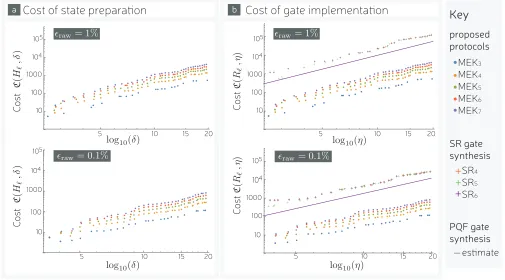
FIG. 5. The resource cost of MEKℓ. (a) shows costC(|Mℓ⟩, δ) of preparing a magic state|Mℓ⟩at error rateδ. (b) shows cost
C(Rℓ, η) of performing a non-CliffordRℓat error rateη. For comparison, (b) also shows the cost of gate-synthesis using the
protocol of Ref. [11]. Both (a) and (b) use initial error rates ofϵ= 0.01 and ϵ= 0.001 for axial rotations of angleθℓ=π/2ℓ
withℓ= 3,4, . . .7. Smaller rotations and other gate-synthesis protocols are considered later.
We consider the cases of raw error rates ofϵraw= 0.01
and ϵraw = 0.001. The case of higher raw noise is an
important benchmark as it has been widely studied [4, 5, 37], and here we see improvements over gate synthesis. For instance, at δ= 10−15 we find PQF is∼22.5 times more costly than MEK6. However, the lower raw noise
regime ϵraw = 0.001 is in many ways more interesting.
In this regime, the advantage of using MEKℓ is further improved by a slight margin. For instance, at target error rate δ = 10−15 we find PQF is ∼ 24 times more costly
than MEK6, which is a larger factor than in the high
noise regime. This widening gap between gate synthesis and MEKℓ is seen for allℓ and δ. This increase in gap is intuitive because the distillation cost drops with ϵraw,
but theT-count of gate synthesis is independent ofϵraw.
While the high noise regime is widely studied, we next argue that the lower noise regime is also more realistic. Underneath magic state factories is a layer of quantum error correction. The highest known thresholds for error correction are ∼ 1% for the toric code [17, 20–22] and
∼3% for Knill’s model of postselected quantum compu-tation [44]. To prevent astronomical overheads, physical gates must be comfortably below the threshold, and so we assume all physical gates have infidelities well below 1%. Because preparing raw magic states will involve several physical gates, it has often been assumed thatϵrawwill be
higher than the physical gate error rate, maybe even an order of magnitude higher. However, Li [41] has shown that we can probabilistically prepare raw magic states at infidelities of about half the physical control-X gate error, assuming control-X failure is the dominant noise mechanism. We remind the reader that we assume logi-cal level control-X gates are ideal, but beneath the hood of error correction we have very noisy physical control-X gates. All this indicates that ϵraw = 0.001 is a feasible
regime, more plausible than ϵraw = 0.01. As such,
fol-lowing subsections focus on the low-noise regime.
VIII. MAGIC STATE DILUTION
|+ |M
|M+1
ρ+1,
ρ,
2
2
[image:10.612.66.287.55.155.2]zoom in
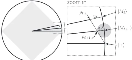
FIG. 6. A geometric representation of the dilution protocol in a cross-section of the Bloch sphere. Note that two points separated by a geometric distance of d in the Bloch sphere, correspond to operators with d/2 distance in 1-norm. The grey diamond shows the set of stabiliser states. Given aρℓ,ϵ
state and a pure|+⟩state we can prepare mixtures on the line between these points. This line intersects the line for states of the formρℓ,ϵ′. We see that for sufficiently largeϵ, the resulting
ϵ′ can be reducedϵ′≤ϵ. Furthermore, we show a 2ϵ′ radius ball about the point|Mℓ+1⟩to highlight that bothρℓ,ϵstate
and|+⟩are further than 2ϵ′away, and so these states would provide a worse approximation of|Mℓ+1⟩than their mixture.
stabiliser state with respect to|Mℓ⟩and find
1
2||(|+⟩⟨+| − |Mℓ⟩⟨Mℓ|)||1=|sin(θℓ)| (21)
∼θℓ=
π 2ℓ,
where the last line gives the small angle approximation. Therefore, the resource becomes free wheneverπ/(2ℓ) is smaller than the target error rate.
We present an alternative solution that keeps us within the framework of diagonal noise and ensures rapid de-crease of costs whenever θ2
ℓ/
√
2 is smaller than the re-quired error rate. This ℓ cutoff is quadratically smaller than that of Duclos-Cianci and Poulin. Letρand ρ′ be
two resource states with costs C and C′. If we choose to generateρwith probabilityλandρ′ with probability 1−λ, then we have the random mixture λρ+ (1−λ)ρ′.
Furthermore, the expected cost is λC+ (1−λ)C′. We consider mixing a noisy|Mℓ⟩state with a|+⟩to obtain a good approximation of a noisy |Mℓ+1⟩state. We say
the state|Mℓ⟩has been diluted, since this allows a source of |Mℓ⟩ states to provide, on average, a greater number of noisy |Mℓ+1⟩ states. We will see that while dilution
may increase noise, there are practically relevant regimes where dilution reduces noise.
We use ρℓ,ϵfor a |Mℓ⟩ state with ϵdiagonal noise, so that
ρℓ,ϵ= (1−ϵ)|Mℓ⟩⟨Mℓ|+ϵ|M¯ℓ⟩⟨M¯ℓ|. (22)
Preparing ρℓ,ϵ costs C(Mℓ, ϵ) resources. The principle result of this section the relation
ρℓ+1,ϵ′ =λρℓ,ϵ+ (1−λ)|+⟩⟨+|, (23)
where
λ= 1
2(1−ϵ), (24)
ϵ′= 1 2
(
1−(1−2ϵ)
[
cos(θℓ) (1−ϵ)
])
. (25)
The dilution providesρℓ+1,ϵ′ at a costλC(Mℓ, ϵ), which
is half the cost of theρℓ,ϵ′ state whenϵis small.
Remark-ably, dilution can even decrease the error rate, provided ℓ is large enough. Specifically, if ℓ is large enough that the fraction in square bracket exceeds 1, then we have ϵ′≤ϵ. A simpler sufficient condition is θ
ℓ≤
√
2ϵ, which can be used to predict a transition in the performance of dilution at
ℓc= log2
(
π
√
2ϵ
)
. (26)
In this regime the cost is halved, and iterating this pro-cess decreases costs exponentially withℓ. However, even whenℓis does not satisfy the above condition, an increase in error rate may still make dilution more efficient than distillation. We give a proof of Eq. (23) in App. E with the underlying geometric intuition presented in Fig. (6).
IX. RESULTS FOR HIGHER ℓ
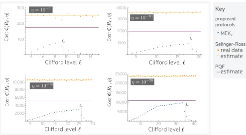
Here we discuss the performance of MEKℓ combined with dilution at performing small angle rotations, be-yondℓ= 7. Our results are generated iteratively. After having compiled a list of achievable costs C(Mℓ, ϵ) and C(Rℓ, η) for different values of ϵ, we next built lists for ℓ+1. The first step is to build a list ofC(Mℓ+1, ϵ′) derived fromC(Mℓ, ϵ) using the dilution protocol in the previous section. Next, we considered different combinations of input states into the MEKℓ, allowing for using diluted states without any further distillation or inputting di-luted states into MEKℓ. The results are presented in Fig. (7) as a function of ℓ, showing how resource costs scale with decreasing angle.
For the target error rates 10−10,10−15,10−20 we can
see three clear regions, with the middle region absent for the 10−5 plot. First, the resource cost increases roughly
linearly with ℓ. Next, there is a transition where the gradient becomes gentler. Lastly, at some cutoff the cost starts to fall exponentially with ℓ. In this last regime, we rely solely on diluting magic states. This exponential cliff was predicted by the analysis in the previous section, and is labeled in the plots byℓc. The behaviour of the middle region is also due to dilution. Here we typically find that one round of MEKℓ is used, with the input noisy |Mℓ⟩ states produced by dilution, as opposed to using two or more rounds of MEKℓ on a raw resource of error rateϵraw. Since dilution is less effective at lowℓ, in
this regime we are completely reliant on MEKℓ and here observe the most rapid increase in costs.
small ℓ, and large ℓ > ℓc there is a significant gain over both gate-synthesis methods by over an order of magni-tude. In the intermediate regime, our protocol still out-performs gate-synthesis but approaches a similar order of magnitude.
X. CONCLUSIONS
We have proposed a protocol for distilling magic states providing small angle rotations at a lower cost than the previous proposal of Duclos-Cianci and Poulin. The cost, as measured by number of raw magic states used, is less than best current gate synthesis techniques. For modest size rotation of angle π/(26), we saw our protocol
oper-ates ∼ 24 times better than gate synthesis. Assessing this improvement, a factor 12 can be attributed to the innovations of Duclos-Cianci and Poulin, with our com-pression of the protocol providing the additional factor 2. To perform smaller angle rotations, the resource cost gradually increases until the resources become close to stabiliser states. To maintain an advantage over gate-synthesis this phenomenon must be exploited. We pro-posed a magic state dilution protocol, which converts one magic state into a larger number suitable for a smaller angle rotation. This exponentially suppresses resource costs for anglesθℓ ≤
√
2ϵ. In this regime, resource costs are many orders of magnitude lower than gate-synthesis. Throughout, we have quantified cost by raw magic states consumed. This is the standard metric in ev-ery paper that has introduced a new protocol for magic state distillation. Other quantities of interest are the to-tal number of qubits used (space cost) and depth of cir-cuits used (time costs). These full resource costs include stabiliser and Clifford costs, but are highly sensitive to the specific architecture used. The fully costed perfor-mance of Bravyi-Haah and Reed-Muller magic state dis-tillation have been considered for surface code architec-tures, both in a braiding picture [7] and using transversal logical gates [18]. Such full resource assessments are sig-nificant undertakings that followed the initial proposals, and so lie beyond our present scope. However, all such analyses to date have found that protocols with lowerT -counts also have lower full resource costs. Although, in Ref. [7] they noted that significant improvements in pro-tocolT counts can lead to more modest improvements of full resource costs. This occurs because the surface code incurs a polylogarthmic overhead inϵ−1that grows more
rapidly than overheads due to magic state distillation or gate-synthesis. That is, in a fully costed analysis the sur-face code overhead dwarfs all other overheads. Though this peculiarity could disappear if future developments provided a more efficient and practical alternative over the surface code.
Here we have considered only single-qubit gate-synthesis, but in parallel work there has been progress on unifying magic state distillation with gate-synthesis for a class of multi-qubit circuits [45, 46]. We close by
remark-ing that the fields of magic state distillation and gate synthesis have rapidly evolved in the last several years, giving good reason to be hopeful that advancement in these areas will continue to bring quantum computation ever closer to reality.
XI. ACKNOWLEDGEMENTS
This work was supported by the EPSRC (grant EP/M024261/1) and collaboration between the authors was facilitated by the NQIT quantum hub. We thank Bryan Eastin and Adam Meier for assistance with re-producing the simulation of MEK. We thank Guil-laume Duclos-Cianci and Mark Howard for comments on the manuscript. Gate synthesis calculations used the Gridsynth package, and we thank Peter Selinger and Neil J. Ross for writing this software and making it available. We thank the developers of the Qcircuit package used in generation of figures. All our analysis is available in the Supplementary material as the Mathematica source files and also in pdf format.
Appendix A: Arbitrary angle rotations
We focus on small angle rotations, but some of our techniques also apply to larger rotations. In particular, not only is Rℓ in the ℓth level of the Clifford hierarchy, butRm
ℓ belongs to the same level for any integerm. For the compressed MEKℓprotocols described we can replace
Rℓ→Rmℓ throughout and they perform identically, and soRm
ℓ has the same resource cost asRℓ.
If we require some rotation with an angleϕthat is not a rational fraction of π, then it will not fall within any level of the Clifford hierarchy. Rather, we may resort to inexact synthesis and find a nθℓ that is sufficiently close toϕ. The larger we choose ℓ, the better the ap-proximation, but the higher the resource cost. Specifi-cally, for allϕ and ℓ we can always find annsuch that
|ϕ−nθℓ| ≤π/2ℓ, which improves exponentially withℓ. To prove this, we observe that for fixed ℓ the set of reach-able angles {nθℓ|1 ≤ n ≤ 2ℓ+1} are equally spaced on the interval [0,2π]. Therefore, the reachable angles have gaps between them of distanceπ/2ℓ. The angle ϕ fur-thest from any angle in the reachable set will sit halfway between two reachable angles, and so this worst caseϕ liesπ/2ℓ+1 away from the nearest reachable angle. For
instance, to ensure|ϕ−nθℓ| ≤10−10we can use ℓ= 35. It is straightforward to verify that high precision in an-gle ensures closeness (upto a constant factor) in diamond norm distance between the corresponding channels.
4 6 8 10 12 14 100
200 300
5 10 15 20
1000 2000 3000 4000
5 10 15 20 25 30 2000
4000 6000 8000 10 000
10 20 30 40
5000 10000 15000 20000 25000
Co
s
t
C
(
R
ℓ
,η
)
Co
s
t
C
(
R
ℓ
,η
)
Co
s
t
C
(
R
ℓ
,η
)
Co
s
t
C
(
R
ℓ
,η
)
Clifford level
Clifford level
Clifford level
Clifford level
η= 10−5
η= 10−10
η= 10−15 η= 10
−20
MEK proposed protocols
Key
Selinger-Ross
real data
estimate
PQF
estimate
c
c
[image:12.612.62.556.52.324.2]c c
FIG. 7. The resource costRℓ rotations using MEKℓ distillation combined with magic state dilution withϵraw = 0.1%. Each plot is for a different final error rateη, and is against the Clifford levelℓbeginning with the first nonClifford levelℓ= 3. We compare perform against gate-synthesis methods, which perform mostly independently ofℓ. For the Selinger-Ross (SR) gate synthesis protocol [11], we show exact data extracted from the gridsynth application and also the analytically proven typical performance. We also show the typical performance for probabilistic quantum circuits with fallback (PQF) [39]. All results here assumeϵraw= 0.001.
to dilution. Therefore, the resource costs presented in Sec. IX only apply whenϕis close to someθℓ.
Appendix B: Precision in gate-synthesis
Across the gate-synthesis literature, different notions of precision are used. Here we discuss how these re-late to the diamond norm measure of noise. We assume throughout that all unitaries are in SU(2) and so have determinant 1.
In Def 7.1 of Ref. [11], SR state that they quantify pre-cision using the spectral norm ϵSR := ||U −V||∞. Let
W = U†V and have eigenvalues exp(iφ) and exp(−iφ)
with φ ≥ 0, so that φ is small whenever U and V are close. It follows that ||U −V||∞ = |1 −exp(iφ)| =
2|sin(φ2)| ∼φ.
IfU andV are channels associated withU andV, then Refs. [47, 48] show the inequality
ϵGS:= 1
2||U − V||⋄≤ ||U−V||∞∼φ. (B1)
We now consider a lower bound. For anyρwith||ρ||1= 1
we have by definition that
1
2||U − V||⋄≥ 1
2||(U ⊗1l)ρ−(V ⊗1l)ρ||1. (B2) Settingρ=|+⟩⟨+| ⊗ |+⟩⟨+|, we find that
1
2||U − V||⋄≥ 1
2|1−exp(i2φ)| (B3) =|sin(φ)| ∼φ
Therefore, in the smallφlimit we have ϵGS=ϵSR. In the work on PQF, they measure precision [49] as follows
ϵP QF :=
√
1−12tr(U†V). (B4)
This evaluates toϵP QF =
√
2|sin(φ/2)| ∼φ/√2. There-fore, this quantity is√2 smaller than our diamond norm measure, so that ϵP QF = ϵGS/
√
a
b
c
|+ • • |+
|0
E R2
E† E
R2
E†
|0
|0 |0
Yx1R
3 Yx3R†
3 Yx
5R
3 Yx7R†
3
Yx2R
3 Yx4R†
3 Hℓ(iY)y Yx
6R
3 Yx8R†
3
|+ • • Zx3+x4+x5+x6 |+
|0
E
R2
E† E
R2
E†
|0
|0 |0
Y(x1+x3)R
3 R†3 R3 Y(x
5+x6)R†
3
Y(x2+x4)R
3 R†3 Hℓ(iY)y R3 Y(x6+x8)R†
3
|+ • Zx3+x4+x5+x6 |+
|0
E E† E E†
|0
|0 |0
Y(x1+x3) Hℓ(iY)y Y(x5+x6)
Y(x2+x4) Hℓ(iY)y Hℓ(iY)y Y(x6+xj)
|+ • Zx3+x4+x5+x6 |+
|0 Yx1+x2+x3+x4+x5+x6+x7+x8 |0
|0 Xx1+x2+x3+x4+x5+x6+x7+x8 |0
X(x1+x3)Z(x2+x4) Hℓ(iY)y X(x5+x7)Z(x6+x8)
X(x1+x3)Z(x2+x4) Hℓ(iY)y Hℓ(iY)y X(x5+x7)Z(x6+x8)
[image:13.612.130.488.54.366.2]d
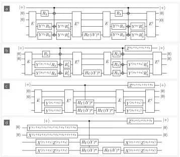
FIG. 8. Propagation noise terms around distillation circuit.
Appendix C: Noise analysis
This section shows how the circuit operates when the non-Clifford gates (R3 and Rℓ−1) are noisy due to
im-perfect magic states. When aRℓgate fails due to noise, it is followed by an additional Y rotation. There are 8 locations that errors can occur on R3 gates and we
de-fine a binary vectorx= (x1, x2, x3, x4, x5, x6, x7, x8) that
records whether aY error occurs at a particularR3gate.
We use the binary variable y = 0,1 to track an error in the pivotal rotationRℓ−1. When theRℓ−1 gate fails, we
have a rotationHℓ(iY) rather thanHℓ. Notice the com-plex phase i, which makes no physical difference to the unitary. However, aspects of the proof rely onHℓ being Hermitian, and the additional phase keeps it Hermitian. The resulting random circuit is shown in Fig. (8a).
We pull some Y noise operators through the control phase gates, which can cause Z noise on the control as shown in Fig. (8b). The central portion of the circuit now contains no noise terms (excepty) and so we can replace it with a logical control (Hℓ⊗Hℓ) or its equivalent when
y= 1. This yields Fig. (8c).
Next, we pull the Y noise backwards through the en-coderE. We already know howEacts on Pauli operators
from which we conclude that the inverse action satisfies
E† :Y3→Y1X2Z3Z4, (C1)
E† :Y4→Y1X2X3X4. (C2)
Similarly random unitariesYα
3 Y
β
4 map as
E† :Yα
3Y4β →Yα +β
1 Xα +β
2 (Z3αX3β)(Z4αX4β) (C3)
Applying this rule to our circuit yields Fig. (8d). From Fig. (8d), we see that to obtain the correct mea-surement outcome on qubit 1 or 2 requires that
|x|:=x1+x2+x3+x4+x5+x6+x7+x8= 0 (mod 2),
(C4) which detects any single error on the R3 gates. This
shows that the error correction properties of our original circuit have survived the compression.
From this circuit we can get some intuition for the leading order error terms presented in Eqs. 13. First consider the failure probability, Pfail = 1−Psuc. If
|x|:=x1+x2+x3+x4+x5+x6+x7+x8= 1 (mod 2),
then we detect an error and have a failure. The leading order contribution is single error processes, and there are 8 such errors, so this contributes 8ϵ3 toPfail. Otherwise,
subspace. This projection detects an errors, and the pro-tocol declares failure if one of the two noisy|Mℓ⟩states is faulty, which occurs with probability 2ϵℓ. Lastly, we consider if everything works except the pivotal rotation. The pivotal rotation fails with probability ηℓ−1, but not
all this contributes to the failure probability. When the pivotal rotation fails, and the rest of the circuit works correctly, it results in the operation shown in Fig. (2c), but with the replacement Hℓ → iHℓY. Algebraically, this operation is
V =1
2[1l + (iHℓY)⊗(iHℓY)] [(iHℓY)⊗1l)] (C5) =−i
2 [(Y Hℓ)⊗1l + 1l⊗(Y Hℓ)]
Applying this channel to |Mℓ⟩|Mℓ⟩, and noting that
Y|Mℓ⟩=|M¯ℓ⟩, we have
|ψ⟩=V|Mℓ⟩|Mℓ⟩=−
i
2 (|M¯ℓ⟩|Mℓ⟩+|Mℓ⟩|M¯ℓ⟩) (C6) Therefore, the probability of an even parity mea-surement, combined with pivotal rotation failure, is ηℓ−1⟨ψ|ψ⟩. Recalling,⟨Mℓ|M¯ℓ⟩= 0, we find⟨ψ|ψ⟩= 1/2. Therefore, the failure probability gains a contribution of
1
2ηℓ−1. This covers all the leading order processes that
contribute to a detected failure.
Next we consider leading order processes that go un-detected, but output an erroneous state |M¯ℓ⟩. The pro-tocol outputs a two qubit state, and we trace out the sec-ond qubit and evaluate the error rate on the first qubit. Switching the first and second output qubit will yield the same result. First we consider pairs of errors in the R3 gates. There are 28 such pairs, all satisfying |x|= 0
(mod 2). However, the parity measurement must yield the correct outcome also. Since we are only considering leading order errors, we can assume the noisy|Mℓ⟩states are error free. Therefore, to obtain the|+⟩on the control ancilla, there cannot be a Z flip on the control, and so x3+x4+x5+x6 = 0 (mod 2). This cuts the number
of undetected error pairs down to 14. Not all undetected error pairs lead to a logical error on the first qubit. For x1=x2= 1 andx7=x8= 1 we see that there is a
logi-calY ⊗Y error, and so both these processes contribute. For the other 12 undetected errors, the parity projection becomes deformed so that it projects onto a state that on average has 1/2 overlap with|Mℓ⟩. Let us expand on this notion of a deformed parity projection by considering the casex1=x5= 1, with other combinations proving
simi-lar. This causes anX⊗X rotation both before and after the parity projection, so that instead of projecting onto Hℓ⊗Hℓwe project ontoHℓ⊥⊗Hℓ⊥whereHℓ⊥:=XHℓX, which we call a deformed projection. How much this par-ticular process contributes varies withθℓ, but a lengthily evaluation over all such error pairs shows the average con-tribution is 1/2. This totals the error contribution from failed R3 gates to (2 + 122)ϵ32 = 8ϵ23. If the R3 gates do
not fail, but instead we have a perfect parity projection, then a logical error occurs if the projection is applied to
|M¯ℓ⟩|M¯ℓ⟩, which occurs with probability ϵ2ℓ. Lastly, we contemplate when the pivotal rotation cairres an error. We see from Eqn. (C6) that|⟨M¯ℓ, Mℓ|ψ⟩| = 1/4 and so the this leads to a logical error with probability 1
4δℓ−1.
We remark again that the leading order contribute here is linear, and not quadratically suppressed, and so the pivotal rotation must be high fidelity to enable distilla-tion.
Appendix D: Generic noise
Throughout the main text, we assumed diagonal noise as described in Sec. VI A. Here we show that MEKℓ is robust against generic noise, making use of the 1-norm and diamond norm to measure error rates. Specifically, our proof will demonstrate that MEKℓnoise is quadrat-ically reduced, converging towards zero. Our proof will provide an upper bound on the output error rate, rather than the exact expression.
We first consider MEKℓas a quantum channelEacting on two noisyρℓ,ϵℓ states, such that
ϵℓ:= 1
2||ρℓ,ϵℓ−ρℓ||1. (D1) where hereρℓ,ϵℓ may not be diagonal in the{|Mℓ⟩,|M¯ℓ⟩} basis. For brevity, we useρℓ:=ρℓ,0=|Mℓ⟩⟨Mℓ|. Below, we also use ∆ℓ:=ρℓ,ϵℓ−ρℓ where||∆ℓ||1= 2ϵℓ.
The protocol uses 8 ρ3,ϵ3 states, which by Clifford twirling arguments can be forced to have purely diag-onal noise. We usex={x1, . . . x8} to label define Pauli
errors from theρ3,ϵ3 states, so that ρ⊗83,ϵ3 =
∑
x∈Z8 2
pxY[x]ρ⊗83 Y[x], (D2)
whereY[x] :=⊗jY xj
j and
px:=ϵ
|x|
3 (1−ϵ3)8−|x|, (D3)
with |x| := ∑
jxj. For a given error configuration x, the protocol implementsEx. We decompose this asEx=
E′′
x ◦ Pℓ−1◦ Ex′, wherePℓ−1 is the noisy pivotal rotation,
E′
x is the circuit before the pivotal rotation andEx′′is the circuit afterwards. Throughout, we use the symbol◦ to denote composition of channels. Lastly we trace out one of the qubits, using the partial trace map tra, to give the single qubit output. The trace is over either qubita= 1 or a = 2, and our analysis will be independent of this choice.
The complete channel is
E=∑
x
pxtra◦ Ex′′◦ Pℓ−1◦ Ex′. (D4)
Next, we use that since 12||Pℓ−1 − Uℓ−1||⋄ = ηℓ−1, we
Dis not necessarily a positive map. This entails
E=
( ∑
x
pxtra◦ Ex′′◦ Uℓ−1◦ Ex′
)
(D5)
+
( ∑
x
pxtra◦ Ex′′◦ D ◦ Ex′
)
.
Recall from Eq. (C4) that the termsE′′
x◦ Uℓ−1◦ Ex′ vanish whenever xhas an odd number of 1s. For the nonvan-ishing xvalues, we split the first bracket into two com-ponents, representing thex= (0,0, . . . ,0) term and then the nonzero|x|= 2,4,6,8 terms
E=p0tra◦ E0′′◦ Uℓ−1◦ E0′ (D6)
+
∑
|x|=2,4,6,8
pxtra◦ Ex′′◦ Uℓ−1◦ Ex′
+ηℓ−1
( ∑
x
pxtra◦ Ex′′◦ D ◦ E
′
x
)
.
We next introduce some new notation to simplify this expression to
E =A+B+C. (D7)
where our new maps are
A= tra◦p0E0′′◦ Uℓ−1◦ E0′, (D8)
B= tra◦
∑
|x|=2,4,6,8
pxEx′′◦ Uℓ−1◦ Ex′
, (D9)
C= tra◦
∑
x
pxEx′′◦ D ◦ Ex′. (D10)
One can easily verify the channels satisfy
||A||⋄≤pg:=p0= (1−ϵ3)8, (D11)
||B||⋄≤pb:=
∑
x=2,4,6,8
(8
x
)
ϵ|3x|(1−ϵ3)8−|x|, (D12)
||C||⋄≤2ηℓ−1. (D13)
Later we also make use of (assumingϵ3 ≤0.01) the
fol-lowing
1−8ϵ3≤pg≤1 (D14) 28ϵ23−168ϵ33≤pb≤28ϵ23 (D15)
We next consider the effect of these channels individually before composing the results together.
TheAmap represents a perfect parity projection with no errors, so that
A(ρℓ⊗ρℓ) =pgtra[ρℓ⊗ρℓ] =pgρℓ. (D16) We consider its action on a noisy stateρℓ,ϵℓ =ρℓ+ ∆ℓ. In the|Mℓ⟩basis we have
∆ℓ=ϵℓ
(
−a b b∗ a
)
. (D17)
From ||∆ℓ|| = 2ϵℓ, we deduce 0≤ |a|2+|b|2 ≤ 1. Per-forming the parity projection on single error terms yields
A(ρℓ⊗∆ℓ) =−pgaϵℓtra[(ρℓ⊗ρℓ)] =−pgϵℓaρℓ (D18)
A(∆ℓ⊗ρℓ) =−pgaϵℓtra[−(ρℓ⊗ρℓ)] =−pgaϵℓρℓ(D19) Lastly for the double error term we have
A(∆ℓ⊗∆ℓ) =pga2ϵ2ℓ[ρℓ+ (Y ρℓY)] (D20) Combining Eq. (D16), Eq. (D18) and Eq. (D20), we have that
A(ρℓ⊗ρℓ) =pg[(1−aϵℓ)2ρℓ+ (aϵℓ)2(Y ρℓY)], (D21) where−1≤a≤1.
TheBmap represents when the pivotal rotation works perfectly, but at least twoρℓ,ϵ3 states cause an error. By elementary norm properties we have
||B(ρℓ,ϵℓ⊗ρℓ,ϵℓ)||1≤ ||B||⋄· ||ρℓ,ϵℓ⊗ρℓ,ϵℓ||1≤pb. (D22) We defineρB:=B(ρℓ⊗ρℓ), and since Bis a completely positive channel we have that tr[ρB] =||ρB||1.
Lastly, theC map represents a failed pivotal rotation. We defineρC :=C(ρℓ,ϵℓ⊗ρℓ,ϵℓ) and use norm properties to deduce||ρC||1≤2ηℓ−1. SinceC is not a positive map,
all we know regarding the trace is that−2ηℓ−1≤tr[ρC]≤
2ηℓ−1.
Putting all these components together we have that
E[ρℓ,ϵℓ ⊗ρℓ,ϵℓ] =pg[(1−aϵℓ)
2ρ
ℓ+ (aϵℓ)2(Y ρℓY)] (D23) +ρB+ρC
Taking the trace gives the success probability
Psuc=pg(1−2aϵℓ+ 2a2ϵ2ℓ) + tr[ρB] + tr[ρC]. (D24)
The smallest value this can take is when tr[ρB] = 0,
tr[ρC] = −2ηℓ−1, and a = 1. This gives the rigorous,
albeit pessimistic bound, that
Psuc≥pg(1−2ϵℓ+ 2ϵ2ℓ)−2ηℓ−1. (D25)
We renormalise to obtain
ρout= 1 PsucE
[ρℓ,ϵℓ⊗ρℓ,ϵℓ]. (D26)
The output error rateδℓ:= 12||ρout−ρℓ||1is then
δℓ= 1 2Psuc
[pg(1−aϵℓ)2−Psuc]ρℓ (D27) +pg(aϵℓ)2(Y ρℓY) +ρB+ρC
1
.
Using the triangle inequality we obtain
δℓ≤|
pg(1−aϵℓ)2−Psuc|+pg|aϵℓ|2+||ρB||+||ρC||
2Psuc
(D28)
≤ pga
2ϵ2
ℓ+||ρB||+||ρC||
Psuc
≤ pga
2ϵ2
ℓ+pb+ 2ηℓ−1
The worst case scenario is again thata= 1, so that
δℓ≤
pgϵ2ℓ+pb+ 2ηℓ−1
pg(1−2ϵℓ+ 2ϵ2ℓ)−2ηℓ−1
. (D29)
Using the worst case bound onpgandpbfrom Eq. (D14), we have
δℓ≤
ϵ2
ℓ+ 28ϵ23+ 2ηℓ−1
(1−8ϵ2
3)(1−2ϵℓ+ 2ϵ2ℓ)−2ηℓ−1 ∼
ϵ2ℓ+28ϵ23+2ηℓ−1,
(D30) where the last approximation gives the leading order terms, showing quadratic suppression inϵℓ andϵ3. This
completes our proof that MEKℓsuppresses generic noise. We remark that though quadratic the prefactor of ϵ3
is 3.5 times larger than in Eq. (13) and Eq. (F1), and the prefactor of ηℓ−1 is 8 times larger. However, these
increased prefactors are mainly artefacts of approxima-tions made in the proof. We report that we also found a proof with a leading order approximationϵ2
ℓ+ 8ϵ23+ηℓ−1,
though the proof is much longer.
Appendix E: Dilution proof
Here we verify the dilution expression in Eq. (23). As an intermediately step in our proof, we begin by consid-ering the mixture 12(ρℓ+|+⟩⟨+|). The pure magic state
ρℓcan be expanded in the Pauli basis as
ρℓ= 1
2(1l +Hℓ) (E1)
= 1
2(1l + cos(θℓ−1)X+ sin(θℓ−1)Z),
and|+⟩⟨+|= 1
2(1l +X). Therefore, in the Pauli basis
(ρℓ+|+⟩⟨+|)
2 =
1
2(1l +q(cos(ϕ)X+ sin(ϕ)Z)), (E2)
where we introduce the variablesq andϕas follows
q= 1 2
√
(cos(θℓ−1) + 1)2+ sin(θℓ−1)2, (E3)
sin(ϕ) = sin(θℓ−1) 2q .
Using standard trigonometric identities, we find
q= cos(θℓ), (E4)
ϕ= 2θℓ−1=θℓ.
This entails
ρℓ+|+⟩⟨+|
2 = cos(θℓ)ρℓ+1+ (1−cos(θℓ)) 1l
2, (E5) =ρℓ+1,sin2(θ
ℓ+1).
where in the last line we have used (1−cos(θℓ))/2 = sin2(θℓ+1). Let us recap. By 50-50 mixing a pure magic
state|Mℓ⟩with a pure|+⟩state, we obtain a noisy|Mℓ+1⟩
state with error rate sin2(θℓ+1). Next, we extend the
proof to account for noise on the initial magic state. Given a noisy magic stateρℓ,ϵ, this can be decomposed as
ρℓ,ϵ= (1−2ϵ)ρℓ+ϵ1l. (E6)
Mixing this with the|+⟩stabiliser state by an amountλ, gives
λρℓ,ϵ+ (1−λ)|+⟩⟨+|=λ(1−2ϵ)ρℓ+ (1−λ)|+⟩⟨+|+λϵ1l. (E7) We chooseλso that the coefficients ofρℓ and|+⟩⟨+|are equal, which requires
λ= 1
2(1−ϵ). (E8)
This yields
λρℓ,ϵ+ (1−λ)|+⟩⟨+| (E9)
= (1−2ϵ) 1−ϵ
[ρ
ℓ+|+⟩⟨+| 2
]
+ ϵ1l 2(1−ϵ).
We can now apply Eq. (E5) to the terms in the square brackets, so that
λρℓ,ϵ+ (1−λ)|+⟩⟨+| (E10)
= cos(θℓ)(1−2ϵ)
1−ϵ ρℓ+1,0+
(1−cos(θℓ))(1−2ϵ) +ϵ 2(1−ϵ) 1l,
which can be more compactly written as
λρℓ,ϵ+ (1−λ)|+⟩⟨+|=ρℓ+1,1−q′
2
, (E11)
where
q′ = cos(θℓ) 1−2ϵ
1−ϵ = cos(θℓ) 1−2ϵ
1−ϵ . (E12)
The most relevant quantity to report is the error rate ϵ′= (1−q′)/2, which follows immediately from the above
as given by Eq. (25).
Appendix F: Simulation results
Using Mathematica, we symbolically simulate the cir-cuit in Fig. (8d). Full details are available in the Supple-mentary material (see MEKL simulation.nb).
We find the output states are again diagonal in the
δℓ= 1 Psuc
(
8ϵ23+ϵ2ℓ+ 1
4ηℓ−1−2ηℓ−1ϵ3+ 6ηℓ−1ϵ
2
3−48ϵ33−8ηℓ−1ϵ33+ 136ϵ34+ 4ηℓ−1ϵ43−224ϵ53+ 224ϵ63 (F1)
−128ϵ73+ 32ϵ83+ϵ2ℓ−ηℓ−1ϵℓ2−8ϵ3ϵ2ℓ+ 8ηℓ−1ϵ3ϵ2ℓ+ 24ϵ
2
3ϵ2ℓ−24ηℓ−1ϵ23ϵ2ℓ−32ϵ
3
3ϵ2ℓ+ 32ηℓ−1ϵ33ϵ2ℓ + 16ϵ43ϵ2ℓ−16ηℓ−1ϵ43ϵ2ℓ
)
,
Psuc=448ϵ53−448ϵ63+ 256ϵ73−64ϵ83+ 1/2ηℓ−1(1−2ϵ3)4(1−2ϵℓ)2+ 2ϵℓ−2ϵ2ℓ (F2) + 64ϵ33(2−ϵℓ+ϵ2ℓ)−32ϵ
4
3(9−ϵℓ+ϵ2ℓ) + 8ϵ3(1−2ϵℓ+ 2ϵ2ℓ)−8ϵ
2
3(5−6ϵℓ+ 6ϵ2ℓ).
[1] B. Eastin and E. Knill, Phys. Rev. Lett. 102, 110502 (2009).
[2] A. Y. Kitaev, A. Shen, and M. N. Vyalyi,Classical and quantum computation, Vol. 47 (American Mathematical Society Providence, 2002).
[3] S. Bravyi and A. Kitaev, Phys. Rev. A71, 022316 (2005). [4] A. M. Meier, B. Eastin, and E. Knill, Quant. Inf. and
Comp.13, 195 (2013).
[5] S. Bravyi and J. Haah, Phys. Rev. A86, 052329 (2012). [6] C. Jones, Phys. Rev. A87, 042305 (2013).
[7] A. G. Fowler, S. J. Devitt, and C. Jones, Scientific re-ports3, 1939 (2013).
[8] V. Kliuchnikov, D. Maslov, and M. Mosca, Physical re-view letters110, 190502 (2013).
[9] A. Paetznick and K. M. Svore, Quantum Information & Computation14, 1277 (2014).
[10] D. Gosset, V. Kliuchnikov, M. Mosca, and V. Russo, Quantum Information & Computation14, 1261 (2014). [11] N. J. Ross and P. Selinger, arXiv preprint
arXiv:1403.2975 (2014).
[12] M. Amy and M. Mosca, arXiv preprint arXiv:1601.07363 (2016).
[13] J. T. Anderson, G. Duclos-Cianci, and D. Poulin, Phys. Rev. Lett. 113, 080501 (2014).
[14] H. Bombin, arXiv preprint arXiv:1311.0879 (2013). [15] H. Bombin and M. A. Martin-Delgado, Physical review
letters97, 180501 (2006).
[16] H. Bombin, R. W. Chhajlany, M. Horodecki, and M. A. Martin-Delgado, New Journal of Physics 15, 055023 (2013).
[17] R. Raussendorf, J. Harrington, and K. Goyal, New Jour-nal of Physics9, 199 (2007), quant-ph/0703143. [18] J. O’Gorman and E. T. Campbell, arXiv preprint
arXiv:1605.07197 (2016).
[19] B. J. Brown, N. H. Nickerson, and D. E. Browne, Nat Commun7(2016).
[20] C. Wang, J. Harrington, and J. Preskill, Annals of Physics303, 31 (2003).
[21] R. Raussendorf and J. Harrington, Phys. Rev. Lett.98, 190504 (2007).
[22] A. G. Fowler, A. C. Whiteside, A. L. McInnes, and A. Rabbani, Physical Review X 2, 041003 (2012). [23] H. Anwar, E. T. Campbell, and D. E. Browne, New
Journal of Physics14, 063006 (2012).
[24] E. T. Campbell, H. Anwar, and D. E. Browne, Phys.
Rev. X2, 041021 (2012).
[25] E. T. Campbell, Phys. Rev. Lett.113, 230501 (2014). [26] H. Dawkins and M. Howard, Physical review letters115,
030501 (2015).
[27] A. J. Landahl and C. Cesare, arXiv preprint arXiv:1302.3240 (2013).
[28] D. Gottesman and I. L. Chuang, Nature402, 390 (1999). [29] S. Lloyd, Science273, 1073 (1996).
[30] D. Poulin, M. B. Hastings, D. Wecker, N. Wiebe, A. C. Doherty, and M. Troyer, arXiv preprint arXiv:1406.4920 (2014).
[31] C. J. Trout and K. R. Brown, International Journal of Quantum Chemistry115, 1296 (2015).
[32] D. Wecker, M. B. Hastings, N. Wiebe, B. K. Clark, C. Nayak, and M. Troyer, Physical Review A92, 062318 (2015).
[33] M. B. Hastings, D. Wecker, B. Bauer, and M. Troyer, Quantum Information & Computation15, 1 (2015). [34] C. Jones, Physical Review A87, 022328 (2013). [35] B. Eastin, Physical Review A87, 032321 (2013). [36] A. Paetznick and B. W. Reichardt, Phys. Rev. Lett.111,
090505 (2013).
[37] G. Duclos-Cianci and D. Poulin, Phys. Rev. A91, 042315 (2015).
[38] D. Gottesman and I. Chuang, Nature402, 390 (1999). [39] A. Bocharov, M. Roetteler, and K. M. Svore, Physical
Review A91, 052317 (2015).
[40] A. Bocharov, M. Roetteler, and K. M. Svore, Phys. Rev. Lett.114, 080502 (2015).
[41] Y. Li, New Journal of Physics17, 023037 (2015). [42] The Gridsynth package is available at
http://www.mathstat.dal.ca/ selinger/newsynth/. [43] Duclos-Cianci, private communication.
[44] E. Knill, Nature434, 39 (2005).
[45] E. T. Campbell and M. Howard, arXiv preprint arXiv:1606.01906 (2016).
[46] E. T. Campbell and M. Howard, arXiv preprint arXiv:1606.01904 (2016).
[47] D.-S. Wang, D. W. Berry, M. C. de Oliveira, and B. C. Sanders, Phys. Rev. Lett.111, 130504 (2013).
[48] D.-S. Wang and B. C. Sanders, New Journal of Physics
17, 043004 (2015).
![FIG. 4. Comparison of the resource cost of distillation using MEKℓof final error ofδorder approximations [43]](https://thumb-us.123doks.com/thumbv2/123dok_us/7819464.173269/8.612.97.519.52.253/comparison-resource-distillation-using-mekof-nal-ofdorder-approximations.webp)