This is a repository copy of The advantages of using excess returns to model the term structure.
White Rose Research Online URL for this paper: http://eprints.whiterose.ac.uk/116505/
Version: Accepted Version
Article:
Golinski, Adam orcid.org/0000-0001-8603-1171 and Spencer, Peter
orcid.org/0000-0002-5595-5360 (2017) The advantages of using excess returns to model the term structure. Journal of Financial Economics. pp. 163-181. ISSN 0304-405X
https://doi.org/10.1016/j.jfineco.2017.05.001
[email protected] https://eprints.whiterose.ac.uk/ Reuse
This article is distributed under the terms of the Creative Commons Attribution-NonCommercial-NoDerivs (CC BY-NC-ND) licence. This licence only allows you to download this work and share it with others as long as you credit the authors, but you can’t change the article in any way or use it commercially. More
information and the full terms of the licence here: https://creativecommons.org/licenses/
Takedown
If you consider content in White Rose Research Online to be in breach of UK law, please notify us by
The Advantages of Using Excess Returns to
Model the Term Structure
∗†
Adam Goli´
nski
Peter Spencer
Abstract
We advocate the use of excess returns rather than yields or log prices in analysing the risk neutral dynamics of the term structure. We show that under standard as-sumptions, excess returns are affine in the risk neutral innovations in the factors. This framework has several important advantages. First, it allows for an easy estimation of models that are more flexible than theAR(1). Indeed, we estimate models with more
general dynamics, likeARFIMA(p, d, q), almost as easily asAR(1). Second, within our
framework the dimension of the unrestricted model is the same for the AR(1) as it is
for the richer models, and does not expand in line with the state vector as it does in a yield or log price framework. This makes it appropriate to test all of these risk neutral dynamic specifications against the same OLS unrestricted alternative. Our results for
the US Treasury bond market show that the unrestricted model is preferred to the
AR(1) by the Bayesian Information Criterion, but the opposite conclusion is reached
for more flexible models. A final advantage of the excess returns framework is that the pricing errors are much lower than for the equivalent log price system.
JEL classification: G12, C58.
Keywords: term structure, excess return framework, long memory.
∗We are grateful to Karim Abadir, Richard Baillie, John Campbell, Laura Coroneo, Antonio Diaz Perez,
Fabrizio Iacone, Francisco Jareno, Scott Joslin, Peter Phillips, Yongcheol Shin, Rob Taylor, Mike Wickens and to participants at the the 2013 EFMA and WFC conferences for helpful comments. We are also indebted to a referee for exceptionally perceptive and helpful suggestions.
†Goli´nski (corresponding author): University of York, Department of Economics and Related Studies;
E-mail: [email protected];
Spencer: University of York, Department of Economics and Related Studies; E-mail:
1.
Introduction
This paper proposes a novel approach to the term structure of interest rates, which allows
the cross section of returns to be modelled easily without necessarily adopting any specific
model of the risk neutral dynamics, other than to assume them to be linear. We exploit
the fact that absent arbitrage and measurement error, the forward price of any security for
any future period is its risk neutral expectation for that period. Thus it can be used to
replace the risk neutral expectation generated by an autoregressive model in the standard
specification of the cross section, allowing less restrictive dynamic specifications to be used.
It follows that the excess logarithmic return on any security can be viewed as a risk neutral
surprise or innovation plus a Jensen term determined by its volatility. Assuming that these
excess returns have a factor structure, this approach yields an affine model that relates M
excess bond returns that are measured with error toK < M factorinnovations, which can be
represented by excess returns on bond portfolios that are assumed to be measured without
error. The loadings of the excess returns on the factor innovations depend upon the risk
neutral factor dynamics, allowing these to be identified and estimated.
In the absence of no-arbitrage restrictions, this model can be estimated simply by
regress-ing the M excess bond returns on the K factor innovations using Ordinary Least Squares
(OLS).1 ThisM×K model can be restricted by making appropriate assumptions about
arbi-trage opportunities and the risk neutral dynamics. We show that the excess return framework
easily handles ARFIMA processes, which include the various autoregressive (AR), moving
average (MA) and long memory (LM) models that have been used in the literature. MAand
LM models are notoriously difficult to estimate, but are easily handled in the excess returns
framework.2 The unrestricted OLS excess returns model provides a convenient
encompass-1
We show that if that the factor dynamics have unrestricted linear representation (allowing them to be represented as an infinite series of current and lagged risk neutral innovations) and the no-arbitrage restriction that follows from the factor structure is neglected, this generates theM ×K unrestricted benchmark OLS
model of the cross section of returns. In contrast, it seems hard to interpret the unrestrictedOLS yield level
benchmark as a model of the factor dynamics.
2Goli´nski and Zaffaroni (2016) model yields with long memory dynamics using infinite-dimensional state
ing model for testing such restrictions and in particular the first order autoregressiveAR(1)
arbitrage-free specification used extensively in the term structure literature.
As Bams and Schotman (2003) and others have noted, a variant of the excess returns
model can be obtained simply by forward-differencing the standard AR(1) affine term
struc-ture model (ATSM), which relates the M log prices or yields to the values of the K factor
portfolios.3 However, we show that this forward-difference relation only holds for theAR(1)
specification; richer dynamic specifications increase the dimensions of the yield ATSM but
not the returnATSM. For example, if the risk neutral dynamics are second order
autoregres-sive (AR(2)) this doubles the number of lagged state variables in the risk neutral dynamics
and means that the M yields are not properly explained by theK factor portfolios; another
K factors are in principle needed to do this.4 However, working with innovations removes
the second and higher order lags (and, in the case of MA models, lagged error terms) from
the risk neutral dynamics and preserves the M ×K structure of the excess returns model.
This is the key message of this paper: the return or forward-difference format provides a
very convenient framework for testing risk neutral models of the factor dynamics because it
is not necessary to restrict attention to the AR(1) model analyzed by Bams and Schotman
(2003), Bauer (forthcoming), Adrian et al. (2013) and others who use returns data. Moreover,
we find that empirically the measurement errors in the return framework are much smaller
than in the corresponding yield model (see Figure 5). Also, as found by Dai and Singleton
(2000), Duffee (2011a) and Adrian et al. (2013), the yield pricing errors exhibit a large degree
of autocorrelation, which disappears when working with returns (see Table 3). These results
suggest that the latter provides a more powerful framework for asset pricing and model
testing. We use this framework to re-assess the performance ofAR(1) and other ATSMs.
Several researchers have noted that the factor loadings estimated for an AR(1) yield
model are typically very close to those of an unrestricted OLS regression and that the
3
Thus the factor loadings matrices of these systems should in principle be identical. 4
Duffee (2011b) and Adrian, Crump, and Moench (2013) have suggested that the performance of the
AR(1) model might be improved by introducing more factors, but this would also increase the stochastic
measurement errors are only a little larger. Hamilton and Wu (2014) and Duffee (2011a)
compare these specifications and show that the AR(1) restrictions are nevertheless strongly
rejected statistically: the differences between theAR(1) andOLS benchmark are numerically
small but statistically significant. Balduzzi and Chiang (2012) also find strong evidence
against theAR(1)ATSM when testing it against theOLS. These findings reflect the fact that
the pricing errors in the Treasury bond market are very small, which means, as Cochrane and
Piazzesi (2008) observe, that the risk neutral model parameters are very precisely determined,
making data for this market very good at comparing the performance of rival models.
We confirm the rejection of the AR(1) restrictions in our data set but, in a more
con-structive way, we show that richer dynamic models with parameters that are constrained by
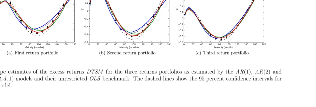
asset pricing theory can beat the unrestricted benchmark model. Figure 2 shows the return
loadings for the AR(1) model alongside the unconstrainedOLS return loadings and their 95
percent confidence interval. As in previous models, the fit looks reasonable, but many of the
AR(1) loadings on the first two factors lie outside the confidence interval. More worrying,
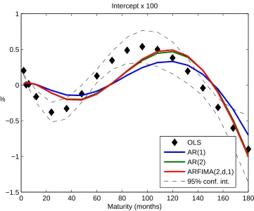
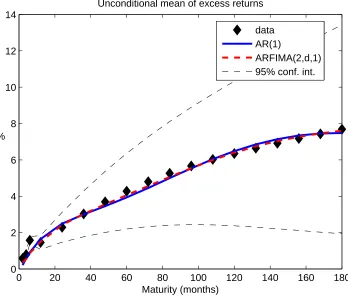
Figure 1 shows that the intercept coefficients of theAR(1) model are visibly and significantly
flatter than those of the OLS benchmark.5 However, the more flexible models do a better
job, generating loadings that largely coincide with the OLS estimates. Reflecting these
ob-servations, on the basis of the Bayesian Information Criterion, the AR(1) specification is
rejected against the OLS benchmark in both yields and returns models, while the AR(2)
returns model is accepted against the benchmark. Further significant improvements in fit
can be obtained by introducing MA and LM factor dynamics as suggested by Fenou and
Meddahi (2009) and Backus and Zin (1993), respectively.
[Insert Figure 1 near here]
[Insert Figure 2 near here]
5
Hamilton and Wu (2014) also find that the badly fitting intercept is the main reason that theAR(1)
Although it is very strong, the statistical rejection of the AR(1) model is very subtle. It
is tempting to think that theAR(1) model could be used for pricing other securities without
incurring economically significant losses. However, Bams and Schotman (2003) provide a
more worrying rejection. They use a fixed effects panel data model to test the three factor
AR(1) model in yields and forward differences and find that although the factor loadings
should be the same, they are visibly as well as statistically very different (see their Figure
5). Our findings echo this result, showing that the loadings of the OLS log price model
differ significantly from those of the OLS returns model. As Bams and Schotman argue,
derivative pricing models based on the two different formulations of the AR(1) model would
give different results, particularly for longer maturities.
The paper is set out as follows. The next section sets out the theoretical model of excess
returns, supported by Appendix A. Section 3 shows how we use conventional yield factor
techniques to make this model operational and derive its likelihood function. Section 4
reports the empirical results and compares them with those from conventional yield models.
Section 5 offers a conclusion and some suggestions for future research.
2.
A Dynamic Term Structure Model for excess
re-turns
This section sets out the theoretical model of excess returns. This is a dynamic term
structure model (DTSM), which combines an ATSM that specifies the cross section under
the risk neutral measure with the return forecasting regression that models the real world
dynamics. We follow Duffee (2011b) in assuming in Section 2 that the returns have an exact
factor structure, before introducing measurement errors in Section 3. That section shows
2.1.
Cross section of excess returns
Let Pm,t be the price of the m−maturity zero coupon bond at time t, pm,t ≡ log(Pm,t)
its natural logarithm and pt = [p1,t, p2,t, . . . , pM,t]′ an M−vector of stacked log prices
representing the cross section. The standardATSM specifies a linear relation between these
log prices (or equivalently, yields) and a set of K < M linear factors zt = [z1,t, z2,t, . . . ,
zK,t]′. The spot rate,rt ≡ −p
1,t, is modelled as the sum of the factors:
rt =µr+1′
zt, (1)
where, assuming that the factors are mean-reverting,µris the risk neutral mean of the short
rate and 1 denotes a vector of ones.
Assumption 1 There are no arbitrage opportunities and there is a risk neutral probability
measure such that each price is equal to the discounted expectation of the price under this
measure.
Assumption 2 The yield curve is spanned by K factors.
The risk neutral expectations of the factors must be unbiased:6
zt=Et−Q1[zt] +uQt , u Q
t ∼i.i.d.N Q
(0,Σ) (2)
whereuQt is aK−vector of mean-zero risk neutral innovations, which we additionally assume
are i.i.d.Gaussian. In this paper we propose an ATSM based on affine relation between the
risk neutral innovations in the log prices and the factors:
pm,t−EQ
t−1[pm,t] =b
′ mu
Q
t , m= 1, ..., M. (3)
Section 3.2 explores the relation between this and the standard AR(1) ATSM.
We can estimate this model by making a few minimal assumptions, consistent with
linearity and the absence of arbitrage. Appendix A shows that because forward prices are
risk neutral expectations in this setting, the log excess return on a bond with maturitym+1,
rxm,t =pm,t−pm+1,t−1−rt−1, is equal to the risk neutral innovation in the log price plus a
convexity term αm:
rxm,t =αm+pm,t−Et−Q1[pm,t]
=αm+b′ mu
Q t .
(4)
The convexity term αm depends on the loadings on the risk neutral innovations in (3):
αm =−1
2b
′
mΣbm (5)
and comes in because we are working with log prices.
We assume that the factors are mean-zero and characterised by the mean-independent
linear representation under the risk neutral measure:7
zk,t =
∞
X
i=0
βk,iuQk,t−i, for k= 1, ..., K, (6)
where uQ
k,t are the i.i.d. Gaussian innovations. This allows the spot rate to be represented
as
rt=µr+
∞
X
i=0
βi′u Q
t−i, (7)
where βi = [β1,i, . . . , βK,i]′.
Assumption 3 Under the risk neutral probability measure the term structure factors have
Gaussian linear dynamics and are mean-independent.
7In other words, as in Joslin, Singleton, and Zhu (2011), the factors have independent dynamics but their
Appendix A shows that the factor innovation loadings in (4) satisfy
bm =−
Xm−1
i=0 βi. (8)
The cross section of M excess returns (4) can be stacked and represented in vector notation
as:
rxt=α+B′uQt , (9)
with B=[b1, . . . ,bM] and, in the absence of arbitrage,
α=−1
2Diag(B
′
ΣB), (10)
where for any square matrix S, Diag(S) is the column vector formed from its diagonal
elements.
2.2.
Return forecasting regressions
Under the real world measureP excess returns are not necessarily mean-zero white noise.
We allow for this by changing measure and specifying the difference between the risk neutral
(uQ
t ) and real world (ut) innovations as:
uQ
t =ut+Σ′λt−1, (11)
where the K−vector λt contains the ‘prices of factor risk’.8 These are specified following
Duffee (2002) as:
Σ′λt=λ0+Λ′1xt, (12)
wherext is potentially an (K+N)−vector of risk factors. These can include theK principal
components of yields that span the term structure as well as N macroeconomic and other
variables that are unspanned, meaning that they affect future returns but not current yields
(Joslin, Priebsch, and Singleton (2014)). Substituting (11) and (12) into (9) gives the return
forecasting regressions (RFRs):
rxt = α+B′λ0+B′Λ′1xt−1+B′ut, (13)
where ut ∼ N(0,Σ).
The details of the change of measure are set out in Appendix B. (9) and (13) constitute a
complete DTSM.
Assumption 4 Under the real world probability measure there can be factors that are not
spanned by the term structure of interest rates but are correlated with the term structure
factors.
3.
The econometric specification
This section shows how we model the risk neutral dynamics using conventional yield
factor techniques to make the excess returns model operational.
3.1.
An approximate factor model
Our theoretical model assumes that the excess returns have an exact factor structure and
can be explained by K risk neutral shocks (9). However, in practice this model is unlikely
to fit perfectly, because bonds are mis-priced or their prices are observed with measurement
error. There may also be model misspecification errors, due to arbitrage opportunities or the
use of an inappropriate model of the dynamics. To allow for this we follow Duffee (2011b),
approximate factor structure which includes so-called return pricing errors vt.9 These are
assumed to be Gaussian with zero mean:
rxot =rxt+vt =α+B′uQt +vt, (14)
where vt∼i.i.d.N(0,Ξ)
and E(vt|uQt ) =0.
Assumption 5 Bond returns are measured with independent and identically distributed
Gaussian measurement errors that are independent of the factor innovations.
Because these pricing errors are not part of the formal model of Section 2, they are
not priced. Thus, they have the same distribution under both the risk neutral and real
world probability measure. The factor model assumes that they are orthogonal to the factor
innovations. Also, for convenience, we assume that they have a zero conditional mean.
To estimate the model we assume that excess returns on K bond portfolios are observed
without measurement error. The portfolio weights are derived from an analysis of principal
components of yields. We select the first K principal components of yields, qy,t = W′yt,
whereytis a vector of yields with the same maturities asptandWis a matrix of eigenvectors
or holdings that defines these portfolios. Applying this matrix to (14) gives the excess returns
on these portfoliosqx,t:
qx,t=W′rxot =αW+B
′ Wu
Q t +W
′
vt. (15)
whereαW =W′α,B′
W =W
′B′. We assume that these excess return portfolios are measured
without error (W′
vt=0) and can be used as observable factor innovations.
9These measurement errors are small but play a non-trivial role, allowing the cross section to be
Assumption 6 There existK portfolios of bond log excess returns that are measured without
error.
We can then back out the set of unobservable factor innovations uQ t :10
uQt =B ′−1
W (qx,t−αW), (16)
Substituting (16) back into (14) gives the ATSM:
rxot = (I−B ′
B′−1 W W
′
)α+B′BW′−1qx,t+vt. (17)
Pre-multiplying (13) by the principal component weights W′ (and using again W′v t = 0)
gives our factorRFRs:
qx,t =c+Cxt−1+et, (18)
et∼N(0,Ω).
where: c = αW +B′
Wλ0, C = B′WΛ ′
1, et = B′Wut and Ω = B′WΣBW. Since c and C
are unrestricted (maximally flexible in the terminology of Joslin et al. (2011), henceforth
JSZ), the Zellner (1962) theorem allows us to estimate them by OLS.We denote theseOLS
estimates asˆc and Cˆ. The price of risk parameters λ0 and Λ1are just-identified and can be
backed out separately. Like the model of the cross section, this RFR system (18) could be
estimated as a stand-alone model. However we estimate it jointly with the model of the
cross section (17), exploiting the fact that the variance matrix Σ is the same under both
measures. The likelihood function of the DTSM is set out in Section 4.2.
10
Invertibility ofBW implicitly depends on the assumption that the factors have distinct dynamics. Joslin
3.2.
Restricting the risk neutral factor dynamics
Unrestricted OLS estimates of theATSM (9) provide unrestricted estimates of the bk,m
coefficients that can be differenced using (8) to retrieve the parameters βk,m of the
un-restricted impulse responses (6). This model is the most general specification satisfying
Assumptions 2-6. We now specialise this using ARF IM A models to represent the loadings
bk,m and using Eq.(10) to make the model arbitrage-free and thus satisfy Assumption 1.
3.2.1. The autoregressive process of order p
In our model the latent factors zt are mean-zero and mean-independent, described by
the MA representation (6). In the AR(1) model the MA coefficients decline exponentially:
βk,i = βi
k. In the absence of repeated roots, each of these components can be integrated to
return the risk neutral factor dynamics:
zk,t=EQ
t−1[zk,t] +u
Q
k,t, k = 1, ..., K, (19)
where:
EQ
t−1[zk,t] =βkzk,t−1. (20)
Stacking these gives:
EQ
t−1[zt] =K1zt−1, (21)
whereβk is thek−th diagonal element of theK×K diagonal matrixK1. This specification
makes zero coupon bond prices log-linear in the levels of the factors:
pt=a+B′zt. (22)
JSZ and others assume that the first K principal components of yields qy,t =W′yt are
the latent factors to be represented by a rotation similar to ours in (16):11
zt=B′−W1(qy,t−αW). (23)
Forward differencing (22) then gives the excess returns relation (9). The intercept coefficients
are lost in this transform but the loadings matrices B in the log price and excess return
representations are in principle identical as noted by Bams and Schotman (2003). The
AR(1) model is unique in this respect. For example, consider theAR(2) model:
Et−Q1[zt] =K1zt−1+K2zt−2, (24)
whereztis still theK×1 vector of current state variables andK1 andK2 areK×K diagonal
matrices. This can be written in a companion form as a restricted 6 factor AR(1) model:
zt
zt−1
=
K1 K2
I 0 zt−1
zt−2
+ u Q t 0
, (25)
The second superrow of this system incorporates a dynamic identity, which makes it less
flexible than an unrestricted 6 factor AR(1) model. Given our other assumptions, it can be
shown that the log bond prices are affine in the state vector zt and its lagged value:
pt =a+B′1zt+B′2zt−1, (26)
where B1 and B2 depend upon K1 and K2 (see e.g. Ang and Piazzesi (2003)). Relaxing
these restrictions would give a conformable OLS encompassing model with 2K ×M free
loading parameters. Naturally, the dimension of the model increases in proportion to that of
11
Although JSZ specify their model in terms of yields rather than returns, our model frameworks are in other respects similar. We both use factors that are mean-independent under the risk neutral measure. Like their VAR model of the real world dynamics, the RFRs that we use to handle the price of risk are
unrestricted and estimated byOLS at a preliminary stage, greatly reducing the number of parameters that
the state vector, which is an undesirable feature when it comes to model selection. However,
forward-differencing has the effect of removing the higher order lags from anyAR(p) system:
pt−Et−Q1[pt] =B′1 zt−Et−Q1[zt]
=B′
1u
Q
t . (27)
Thus, for more general dynamics thanAR(1), the loading matrixBfor prices in (22) will be
misspecified and will, in principle, differ from the loading matrix for excess returns in (27).
3.2.2. Autoregressive fractionally integrated moving average models
In addition to the AR class of models, we also consider the more general autoregressive
fractionally integrated moving average ARFIMA(p, d, q) model (see Granger and Joyeux
(1980), Hosking (1981)):
Φk(L) (1−L) dk
zk,t = Θk(L)uQk,t, k= 1, ..., K, (28)
where Φk(L) and Θk(L) are polynomials of orderpand q, respectively, dis the long memory
parameter and L is the lag operator. This allows us to specify (6) as:
βk(L)uQ
k,t = Φk(L)
−1(1−L)−dk
Θk(L)uQk,t. (29)
The process is stationary if the autoregressive roots lie outside the unit circle and the long
memory parameter is smaller than 1/2. For example, theARFIMA(2, d,2) process with zero
mean for zk,t is given by:
1−φk,1L−φk,2L2
(1−L)dk
zk,t = 1 +θk,1L+θk,2L2
To specify the values ofβk used in estimation as a function of ARFIMAparameters we first
note that:
(1−L)−dk
= 1 +dkL+dk(dk+ 1)L2/2! +dk(dk+ 2) (dk+ 3)/3! + . . . , (31)
which can be substituted (together with similar expansions of Φk(L)and Θk(L) in terms of
L) into (29). The β′s are then determined by matching the coefficients on both sides of (29)
at each lag (or power of L). In practice, we only need to compute these coefficients up to
the maximum lag given by the highest maturity of the bond (excess return) in the sample.
This allows the likelihood of the model to be written in terms of the parameters (β) of the
MA process (7) driving the spot rate.
3.3.
The dynamic and stochastic dimensions of an AR model
Because the dimension of the ATSM in returns (9) is not affected by the dynamic
specification, this allows different specifications to be tested against the same parsimonious
(K + 1)×M OLS benchmark. Crucially, we do not lose any information about the risk
neutral factor dynamics using this transform. That is because we can use the Yule-Walker
equations to rewrite any AR model like (24) as a moving average process (6), letting the
βk,mparameters and hence theαm andbm coefficients of (4) depend uponARparameters in
K1 and K2. 12 Maximum likelihood estimates of the latter can then be obtained by fitting
the model to the data and optimizing the likelihood function.
When working with prices rather than returns higher order risk neutral factor dynamics
mean that, besides contemporaneous factor values, their lags are reflected in prices. For
example, the AR(2) model implies that bond prices are affected by both contemporaneous
and once-lagged factor values (26). With K = 3, its companion form (25) is of dimension
6×6, which (after rotation) means that prices could be spanned by six noiseless principal
12
components. However, there is an important distinction from the richerAR(1) model, which
relaxes the dynamic identity: the six factor AR(1) model has a full stochastic span because
it incorporates six factor innovation terms rather than the three incorporated into uQ t in
(25). It would generally take six principal components or other factor portfolios to hedge
any price in this model, whereas three portfolios (held with the weights b′ mB
′−1
W defined in
(4) and (16)), are sufficient in the 3 factor AR(2) model.
3.4.
Identification
We have adopted a series of normalization restrictions to identify the model. First, the
short rate has unit factor loadings, as in JSZ. Second, as in Dai and Singleton (2000),
Single-ton (2006) and JSZ the factor means are assumed to be zero under Q, allowing the central
tendency to be determined by the short rate equation (1). Finally, the factors are ranked
ac-cording to their persistence, as in Hamilton and Wu (2012).13 Other equivalent identification
schemes are possible by invariant transformation (rotation) of the factor dynamics.
We also assume that the factors are mean-independent, as in JSZ. This model is
maxi-mally flexible in the sense of Dai and Singleton (2000)) forAR(1) dynamics (21). However, it
is an over-identifying restriction in richer ARFIMA specifications.14 In other words, it does
not allow for the most general (maximally flexible) specification of the factor dynamics. For
the VAR(2) withK = 3 dynamic model in (24), a maximally flexible specification would
al-low 6 dynamic restrictions. For example, we could folal-low the JSZ rotation and assume that
K1 was unrestricted and K2 diagonal. Although we can handle this in our excess return
framework by allowing in the factor dynamics in (6) to be interdependent, this additional
flexibility would come at a cost of a significant increase in computational complexity. Adding
long memory component would further complicate modelling the dynamics of the system.
As such, we use our ARFIMA specifications with mean-independent factors as a tractable,
13Specifically, the factors in long memory models are ranked in terms of their long memory and in short
although not maximally flexible, generalization of the popularAR(1) model.
3.5.
The relationship with previous models of excess returns
The excess return framework (14) has also been used by Bams and Schotman (2003),
Bauer (forthcoming) and Adrian et al. (2013) to model the cross section under the AR(1)
assumption.15 However, the framework developed in this paper is novel in two respects.
First and foremost, we use the excess return representation to handle higher order
autore-gressive models as well asARFIMAmodels that encompass theARandARMAmodels used
previously in this literature. 16 Second, we use excess returns to model the innovations on
the right as well as the left hand side of (14), mimicking the JSZ assumption that some
portfolios of yields are observed without error by assuming that the returns on these
port-folios are measured without error. This allows us to exploit the consistency between excess
returns that follows from the assumption of no-arbitrage when these have an approximate
factor structure. In contrast, the standard approach completely ignores the information in
the forward rate structure, using the AR(1) specification (21) to model the risk neutral
ex-pectations instead. Bams and Schotman (2003) model the forward difference system on the
right hand side of (14) but use a specific effects panel data model to represent the innovations
uQt, while Bauer (forthcoming) uses macro ‘news’ to do this.
Like Bams and Schotman (2003) and Bauer (forthcoming) we model the cross section
under the risk neutral measure, exploiting the precision given by the small pricing errors. In
contrast, Adrian et al. (2013) estimate the parameters of the system under the real world
probability measureP. Under this measure the excess return on them−period bond in (13)
15Bauer models innovations in forward rates rather than forward log prices, but his specification is similar
to (9).
can be written as:
rxm,t = 1 2b
′
mΣbm+b′m(λ0+ Λ1′xt−1) +b′mut+vm,t (32)
Adrian et al. (2013) adopt theAR(1) assumption, modelling the factorsxt−1 underP using
a vector autoregression (VAR). They fit (32) using residuals from thisVAR to represent the
priced return innovations ut. The regression coefficients on this vector give an estimate of
bm and the other parameters can be estimated using cross-section regressions.17 These can
be used to construct a model of theAR(1) risk neutral dynamics in (21) and hence estimates
of the factor loadings in the ATMS (22).
4.
Estimation method and results
This section presents our results, starting with a description of the data set. It shows how
we use conventional yield factor techniques to make the excess returns model operational and
derive its likelihood function. Our empirical work starts by examining the cross-sectional
behaviour of returns, yields and log prices using (17) and (22). This strongly suggested the
use of return data in subsequent analysis. We next develop a set of RFRs that model the
behaviour of returns under the real world measure P. Then we combine the cross-section
and RFR systems and estimate them jointly as theDTSM.
4.1.
Data
The empirical models are fitted to a monthly data sample extracted from two well-known
data sets. The first is that of Gurkaynak, Sack, and Wright (2007), henceforth GSW. This
has the attractive feature that it allows prices and yields to be generated at any maturity,
17The price of risk parameters λ
which greatly facilitates the calculation of the monthly log forward prices and returns used in
this study.18 Adrian et al. (2013) also use this source to calculate the monthly returns used
in theirRFRs. Because yield data at the long end are thin (issuance of the 30 year Treasury
bond was suspended between 2002 and 2006), we restrict the analysis to maturities up to 15
years. The number of actively traded securities is also sparse at the short end. Moreover,
GSW only employ Treasury bonds in their sample (excluding Treasury bills and notes). They
do not use any bonds with a maturity of less than four months and it is sometimes hard to
reconcile their yield estimates for maturities of less than one year with data for yields on
Treasury bills and notes (which are excluded from their sample). To allow for this we follow
Duffee (2010) and others in taking our short maturity observations from the Fama Treasury
Bill Term Structure Files available from the Center for Research in Security Prices.19 We
also took the data for our one month spot interest rate from this source.
Our cross section of yields and log prices starts at the short end with the 2, 4 and 6
month maturities extracted from the Fama Treasury Bill Term Structure files and adds
those for the annual maturities 1 through 15 from GSW, giving a total of 18 maturities.
Yield portfolios, qy,t, were estimated as the first three principal components of these yields
with weights W given by the eigenvectors corresponding to the three largest eigenvalues of
the yields covariance matrix (qy,t =W′yt). The excess returns on these 18 maturities were
then calculated (rxn,t, with n = 1/6,1/3,1/2,1,2, ...,15 years) and the weightsWwere used
to find the noiseless portfolios of returns (qx,t =W′rxt). In view of a suspected structural
break in the time series behaviour following the end of the Volker experiment in 1982, we
used the estimation period January 1983 to December 2011.20
18Conveniently, this gives the parameters of the interpolated yield curve, allowing us to find bond
returns on a consistent time period/maturity basis. The parameters are available from from http: //www.federalreserve.gov/pubs/feds/2006/200628/feds200628.xls.
19These estimates are obtained using the bootstrap method rather than curve fitting approximations,
which is generally thought to produce more robust estimates at the short end. For a detailed description please see the US Treasury Database Guide at: www.crsp.com/documentation.
20
Figure 3 presents time series for the 1 month, 3 and 15 year maturity yields. It shows the
well-known downward trend in interest rates over the three decades. This trend underpinned
the handsome realized returns on bonds over this period. In Figure 4 we plot the average
annualized 1 month excess returns on zero coupon bonds over the 1 month rate. It reveals
that over our sample period the excess return on the 15 year zero coupon bond was close to
7.7%.21
[Insert Figure 3 near here]
[Insert Figure 4 near here]
4.2.
The likelihood function
The set of variables observable by an econometrician consists of a time series of M excess
returns observable with errors, rxo
t, and K portfolios of these returns that are assumed to
be observed without error, qx,t. Also, an econometrician observes a number of
economy-wide variables, both spanned and unspanned by the bond market, summarized in a vector
of variables xt. The spanned yield curve factors are the first three principal components of
yields, while the unspanned factors are the fourth and fifth principal components of yields
and macro variables. The significance of the conditioning variables inxtis assessed in Section
4.4.
Under these assumptions the parameters of our model can be estimated by joint nonlinear
optimization of the likelihood of (17) and (18). Let Θ ≡ (β,Σ, Ξ, λ0, Λ1) denote the
parameters of the full model where β is a vector of parameters specifying the risk neutral
dynamics βi. Since the model is Gaussian, we estimate it by maximum likelihood (MLE).
Conditional upon the lagged factors xt−1, the log-likelihood function is:
log (L(Θ)) =
T
X
t=1
logf(rxot,qx,t|xt−1; Θ), (33)
where the joint conditional density of the observed period t data can be decomposed into
the likelihood (g) of observing the excess returns given the spanned factors (which is given
by (17)) and the likelihood (h) of observing the latter given the lagged factors (18):
f(rxo
t,qx,t|xt−1; Θ) =g(rxot|qx,t; Θ)×h(qx,t|xt−1; Θ)
=g(rxo
t|qx,t;β,Σ,Ξ)×h(qx,t|xt−1;λ0,Λ1, β,Σ).
(34)
Since the unspanned variables are not traded (either individually or as portfolios) they do
not enter the likelihood function. Our estimation strategy is based on a direct specification
of the risk neutral dynamics and the price of risk. The real world factor dynamics can then
be determined subsequently using the change of measure technique described in Appendix
C.
As usual, the parameters of the measurement error covariance Ξ can be concentrated out
of the first (cross-section) component of (34) and, as noted above, the reduced form estimates
ˆc and Cˆ can be substituted for λ0,Λ1 and β in the second (time-series) component:
f(rxo
t,qx,t|xt−1; Θ) =g∗(rxot|qx,t;β,Σ)×h(qx,t|xt−1;ˆc,Cˆ,Σ,), (35)
Thus, we use numerical methods only to find the maximum likelihood estimates of (β,Σ)
using the conditional densities given by (35). Moreover, as in JSZ, we can use a
transforma-tion of the covariance matrix of the residuals from (18) to obtain a good starting value for
Σ:
Σ=B−1
WΩBb
′−1
W . (36)
our assumption that the excess portfolio returns qx,t are measured without error. This
leaves open the possibility that the portfolios of log bond prices (or yields), qy,t, could
be measured with error. Because we use them as regressors in (18), this would induce
measurement error bias in the RFRs in our framework. However, this is much less of a
problem than errors in qx,t would be. These RFRs are only used in a forecasting guise and
OLS regressions give consistent predictions even if the regressors are observed with error.22
The RFR parameters are only used in a subsidiary exercise to estimate the prices of risk
and hence the P−dynamics, as explained in Appendix C. Moreover, any parameter bias in
the RFRs should be tiny since it depends upon the ratio of the measurement errors to the
prediction errors, which is negligibly small in models of the Treasury market.
4.3.
Preliminary cross-section tests
Our empirical tests start by examining the cross-sectional behaviour of yields, log prices
and returns using a conventional three factor model. At this stage we only consider
cross-sectional restrictions on the risk neutral dynamics in anATSM framework, without imposing
restrictions on the physical dynamics of the factors. Recall that these restrictions mean that
each model of the cross section of returns is linear in variables but subject to nonlinear
restrictions across its coefficients. These models are therefore nested within an unrestricted
OLS benchmark model. Table 1 shows the basic results from these tests. It reports the
log-likelihood for each model, the number of parameters and the Bayesian Information Criterion
value (BIC), which makes a correction for the number of parameters and sample size and
is the basic model selection criterion used in this paper.23,24 Our tables show the negative
22Johnston (1963), pages 290-291. He also notes on page 283 that decision makers are likely to use the
same mis-measured observations as the econometrician, making it reasonable to suppose this is the relevant model, giving a plausible split of the returns into forecastable and unforecastable components.
23The weighting matrix used to calculate observable portfolios is the same for the all models: the three
eigenvectors associated with the first three principal components of yields. 24Naturally, yields are a simple transformation of log prices, y
m,t= (−1/m)pm,t and, as such, it should
not matter if the model is estimated in yields or prices. The difference in our exercise comes from applying the same weighting matrix W to find observable portfolios of yields and prices, respectively. We checked
of the BIC statistic, making it appropriate to select the model with the highest value of
(−)BIC=2 lnL −kln(T M), where, L is the value of the maximized log-likelihood function,
k is the number of parameters and T and M are the numbers of observations in the time
series and cross-sectional dimension, respectively.
[Insert Table 1 near here]
The first panel of the table shows that the yields strongly reject the AR(1) restrictions,
reflecting the results of Hamilton and Wu (2014).25 However the second panel shows that
the difference in the test statistics for log prices is smaller than in the yields model. The
final panel of the table shows that the difference between the AR(1) and OLS models is
even smaller in the returns data, but that the latter is still preferred on the basis of theBIC
selection criterion. Further improvements can be obtained by introducing moving average
or long memory factor dynamics but we investigate these models in using the full DTSM
framework, reporting the results in Sections 4.6 and 4.7 below.
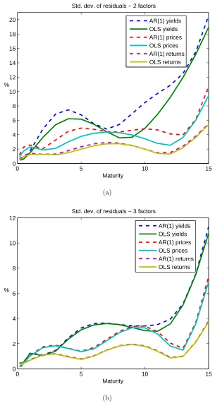
We subsequently re-run these tests using a two factor model. Figure 5 plots the standard
deviations of the residuals of the two factor (Panel A) and three factor models (Panel B)
estimated in yields, log prices and returns.26 Again, it is evident that the restricted AR(1)
yield and log price models have difficulty in matching their unrestricted OLS counterparts.
Although the residuals for the two factor AR(1) yields and log prices are visibly higher than
for theOLS, these differences being much higher than for the three factor tests, the difference
remains tiny for the returns model. Moreover, these residuals are surprisingly small, of the
order of 2−3 basis points in the 1−10 year maturities, hardly any higher than those for
the three factor analogue.
[Insert Figure 5 near here]
25
They test these restrictions within a DTSM framework while our test is for the ATSM cross-section
model. 26
Despite the statistical preference for the OLS over theAR(1) models, the response
coef-ficients for these pairs of models are numerically close in each data set, as we would expect
from previous findings reported in the literature. The standard errors are also small.
How-ever, the coefficients of the models fitted to log prices and returns data are visibly different,
as Bams and Schotman (2003) found for their yield and forward-differenced yield models.
As can be inferred from (3), if the AR(1) models replicate the OLS coefficients accurately
then theOLS coefficients of the log price in (22) and returns (9) models should be the same.
This relation holds also for rotated factors:
pt=Aqp+B′qpqp,t+wt, (37)
and
rxt =Aqx +B′qxqx,t+vt, (38)
where qp,t = W′pt, since the weighting matrix W is the same. In Table 2 we test the
null hypothesis that Bqp = Bqx. Under the alternative hypothesis (Bqp 6= Bqx) the joint
likelihood is the sum of the likelihoods of the two OLS models shown in Table 1 for the
model for prices and returns (39,068.08). We compare this value with that of a joint model
that uses the same slope parameters in both log price and returns data (38,820.81). The
likelihood ratio test rejects the null hypothesis at any conventional significance level. As
noted in Section 3.2, this could indicate dynamic misspecification. The table also shows that
the BIC value for the model under the alternative hypothesis is better than that for the
model under the null.
[Insert Table 2 near here]
It is also worth noting that the volatility of the residuals from the yield and log price
regressions shown in Figure 5, which can be interpreted as pricing errors, is much higher
this could largely be due to the first order autocorrelation in the levels data noted previously
by other authors (Dai and Singleton (2000), Duffee (2011a), Adrian et al. (2013), Hamilton
and Wu (2014)). The autocorrelation in pricing errors can be corrected by first differencing
the data or fitting a time series model to the errors as proposed by Hamilton and Wu.
Switching to a returns or forward difference framework as we propose surely offers a more
natural way of dealing with this problem. Table 3 shows that the return pricing errors are
not significantly autocorrelated, which is consistent with our model assumption. If this were
literally true, this would mean that the bond pricing errors were close to a random walk.27
[Insert Table 3 near here]
4.4.
Modelling the price of risk
Our DTSM amalgamates the models of the returns under the risk neutral and real world
measures (respectively the cross-section (17) and RFR (18) models) and estimates them
jointly subject to the restriction that the innovation variances (Σ) are the same in both
models (see Section 4.2). This section discusses theRFRs for the excess returns on the three
noiseless portfolios qx,t (i.e. those that have returns observed without error, (18)) and the
variables driving the price of risk. The evidence on price of risk factors in the term structure
literature is mixed. Cochrane and Piazzesi (2005, 2008) claim that there is only one pricing
factor driving the risk premium that is not spanned by the first three principal components
of the term structure, which is nonetheless a combination of different yields. Duffee (2011b)
shows that the forth and fifth principal components help to forecast excess bond returns and
similar conclusion is reached by Adrian et al. (2013). Based on this evidence, we initially
included the first five principal components of yields in the xt vector in (18). The work of
Ludvigson and Ng (2009) and Joslin et al. (2014) also suggested the use of macro variables
like industrial production growth (IP) and expected inflation (EI).28
Our preliminary estimation results suggested that the second and third principal
compo-nents of yields as well as expected inflation were insignificant in theRFRs and we therefore
drop these regressors from our final model. Table 4, panel A, reports the estimates of the
RFR parameters for the remaining variables and their significance. There is no obvious
pattern of signs and significance across regressors. Panel B of Table 4 reports the F−test
of joint significance of each variable in the three regressions. It is interesting to note that
although the pricing variables are mostly individually insignificant in particular regressions
their overall effect is very significant.
[Insert Table 4 near here]
4.5.
The risk neutral dynamics in the DTSM
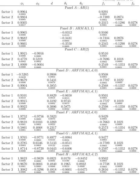
We estimate eight models that maintain Assumptions 1-6, in which the risk neutral
dynamics are restricted using the following specifications: AR(1), ARMA(1,1), AR(2),
ARFIMA(1, d,0),ARFIMA(1, d,1),ARFIMA(2, d,0),ARFIMA(2, d,1) andARFIMA(2, d,2).
In these models we parametrize all three factors in the same way, e.g. for the first model
all three factors have AR(1) dynamics. Table 5 reports the estimates of the risk neutral
parameters of these models. The asymptotic standard errors are reported in a small font.
[Insert Table 5 near here]
All models exhibit very high short memory persistence. The highest autoregressive root
is typically higher than 0.99. The models withAR(2) dynamics also display very high short
memory persistence, with roots larger than 0.99, in the second factor (ARF IM A(2, d,1) and
ARF IM A(2, d,2)) or in all three factors (AR(2) andARF IM A(2, d,0)). The models with
28IP is the monthly logarithmic growth in the seasonally adjusted industrial production index and EI is a
long memory, except forARF IM A(1, d,0), exhibit ‘dual persistence’ under the Q measure:
long-lasting short and long memory dynamics. The values of the long memory parameter
are different for different models. All long memory models, however, have at least one
non-stationary (i.e. withd >0.5) and one stationary (d <0.5) factor. For theARF IM A(1, d,0)
model one factor has a very persistent long memory parameter, just below 1, but its AR(1)
coefficient is negative. The most persistent factor in other models with fractionally integrated
component has long memory coefficient between 0.6 (in theARF IM A(2, d,0) model) and 0.9
(in the ARF IM A(1, d,1) and ARF IM A(2, d,1) models). Generally, the second and third
factors in long memory models also display a significant degree of long range persistence,
between 0.23 and 0.55 (except the third factor in the ARF IM A(2, d,1) model for which
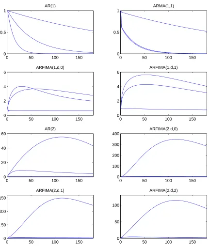
the long memory estimate is close to zero). The factor dynamics under the Q measure are
shown in Figure 6, which plots the moving average representation of the risk neutral factor
dynamics in these models (the β coefficients in (7)). These effects are depicted in the form
of an impulse response function, showing the response over time of the spot rate to a unit
shock spanned by the yield curve.
[Insert Figure 6 near here]
4.6.
The real world dynamics
Appendix C shows how the model of the risk premium (12) is used to obtain the real
world short rate dynamics ((C-8) in this appendix) from the risk neutral short rate dynamics
(7). Figure 7 shows the effect of shocks backed out from the three noiseless portfolios used
as factors (theΦ’s in (C-8)) and is comparable with Figure 6 showing the impulse response
functions under Q. While the general pattern is similar to that of Figure 6, these responses
tend to be smaller and their ‘humps’ more muted, making them look more exponential
than the impulse response functions under Q. Figure 8 shows the effect of the standardized
the evolution of the yield curve but not the current yield curve. As expected, an increase in
industrial production increases the interest rate.
[Insert Figure 7 near here]
[Insert Figure 8 near here]
4.7.
Relative model performance
4.7.1. Likelihood comparisons
The standard errors of the cross-sectional parameters shown in Table 5 are very small.
There are two reasons for this. The first is that the likelihood of the cross section
de-pends upon measurement errors (vt) that are, as Cochrane and Piazzesi say in their 2008
paper, ‘tiny’ empirically, so that restrictions that generate tiny perturbations in the yield
curve estimates are often rejected. The second is the large sample of the panel data, which
tends to bias classical statistics such as likelihood ratio statistics toward rejection of model
simplifications (Hendry (1995), Canova (2007)). The BIC statistics adjust for this effect.
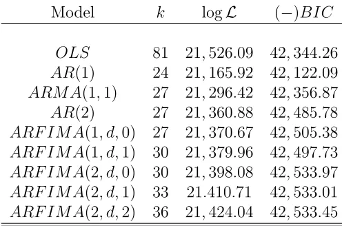
Table 6 reports the number of parameters, log-likelihood andBIC values for each model.
The most striking fact that emerges from this comparison is the very poor explanation of the
data provided by theAR(1) model. Despite the fact that it saves 57 degrees of freedom, it is
the only model that is not preferred to theOLS model on theBIC. Relaxing the tightAR(1)
dynamics results in a big increase in the likelihood function which in turn results in a better
BIC statistic. For instance, adding the moving average component MA(1) or allowing for
AR(2) dynamics increases the likelihood by 130.50 and 194.96, respectively. However, these
short memory models are still inferior to the models with long memory dynamics. The long
memory models perform much better than the rest in this comparison. According to BIC,
theARFIMA(2, d,0) ,ARFIMA(2, d,1) andARFIMA(2, d,2) have very similar performance
[Insert Table 6 near here]
4.7.2. OLS comparisons
Hamilton and Wu (2014) note that the rejection of the AR(1) DTSM against the OLS
benchmark is to a large extent due to its tight restrictions on the intercept terms. If these
are freely estimated the likelihood of the model improves significantly, though not enough to
beat the benchmark. These restrictions stem from Assumption 1 and Jensen’s inequality and
are functions of the moving average coefficients of the factors under the risk neutral measure
(10). Figure 1 plots the intercepts (17) estimated for theAR(1),AR(2), andARFIMA(2, d,1)
models against those of the unrestricted OLS benchmark and its 95% confidence interval.
The estimated coefficients depend on the assumption about the weighting matrix W which
selects the noiseless portfolios. For our particular choice of the first three eigenvectors of
yields, the intercepts have a sinusoidal shape. Evidently, all of these models find it difficult
to replicate theOLS intercepts. However, theAR(2) andARFIMA(2, d,1) model intercepts,
display a visibly better fit than those of the AR(1) ones, especially at the long end. The
AR(1) model produces intercepts that are too flat to fit the OLS model.
Figure 2 plots the loadings (slope coefficients) on the noiseless portfolios in these models.
These loadings also have a sinusoidal shape. As noted by Cochrane and Piazzesi (2008),
the very small errors give a very tight confidence intervals for the loadings. This allows
for a powerful discrimination between particular models, as noted in the previous section.
As is evident from the figures, despite the fact that the AR(1) model yield loadings seem
to be close to those of the OLS model, these coefficients lie outside the 95% confidence
interval for most maturities. The AR(2) and ARFIMA(2, d,1) models are able to replicate
the OLS estimates much better, lying within the confidence interval for most maturities.
Also, the ARFIMA(2, d,1) model fits the slope coefficients slightly better than the AR(2)
model, especially for the first and second portfolios, which is the most likely the reason for
4.7.3. Low frequency characteristics
It is well known that interest rates are highly persistent. Usually the highest
autoregres-sive root estimated for a DTSM is very close to one (see e.g. Bauer, Rudebusch, and Wu
(2014) and references therein). Other researchers attribute the high persistence in interest
rates to fractionally integrated or long memory processes (see for example Gil-Alana (2004),
Iacone (2009), Osterrieder (2013), Goli´nski and Zaffaroni (2016)).
The long range behaviour of yields is best described by the shape of the periodogram
near frequency zero. In Figure 9 we plot the logarithm of the periodogram ordinates of the
standardized first principal component of yields for the first 25 Fourier frequencies. The
periodogram of a series xt is defined as:
I(λ) = 1 2πT
T
X
t=1
xteıtλ
, (39)
where ı denotes a complex unit and the Fourier frequencies are λj = 2πj/T. In the
neigh-borhood of frequency zero the periodogram displays a steep spike, a tell-tale characteristic of
a long memory processes. This is consistent with one of the definitions of the long memory
process, which defines it as having an unbounded spectral density at frequency zero (see e.g.
Baillie (1996), Diebold and Inoue (2001)). On the other hand, a stationary ARMA process
has a bounded spectral density at frequency zero.
[Insert Figure 9 near here]
Although we directly estimate the risk neutral dynamics rather than the physical
dynam-ics, Goli´nski and Zaffaroni (2016), Theorem 4.4, show that in the affine setting, the largest
order of (fractional) integration under the P and Q measures coincide, and this determines
the spectral density of yields at the zero, i.e.:
s(λ)∼cλ−2d
where ∼ denotes asymptotic equivalence andd=max(d1, . . . , dK).
Thus, to examine the ability of particular models to emulate the behavior of the
peri-odogram of yields at ultra-low frequencies, Figure 9 plots the periperi-odogram alongside the
spectral densities of the autoregressive series:
sAR(1) =
(1−φ2) 2π
1−φeıλ−2 (41)
with AR1 coefficientφ= 0.996, and the long memory processes:
sLM(λ) = cλ−2d, (42)
where c is some generic constant. Based on our estimates of long memory parameters, we
plot the spectral density ford= 0.9, which is close to the estimate of the largest long memory
parameter for models ARFIMA(1, d,1) and ARFIMA(2, d,1), and d = 0.7, which is close
to the estimate in the ARFIMA(2, d,2) model. The size of the autoregressive coefficient
corresponds to the typical degree of persistence found in interest rates. It is close to the
highest autoregressive root estimated under the Q measure for the AR(1) model (0.9964)
and slightly higher than the estimate of the autoregressive coefficient for the first principal
component (0.9945). Figure 9 shows that despite the very high short memory persistence
the autoregressive model is not able to match the periodogram ordinates at the lowest
fre-quencies. The long memory models perform much better in this respect. The model with
d = 0.7 matches the lowest frequencies, but it flattens out too quickly for the intermediate
frequencies. It seems that the model with d = 0.9 generates the spectral density that most
5.
Conclusion
The term structure literature has almost invariably modelled the dynamics of the yield
curve as the autoregressive process of order one despite mounting statistical evidence that
this model is misspecified (Duffee (2011a), Hamilton and Wu (2014)). It may be tempting
to think that theAR(1) model is still acceptable since the measurement errors are small and
the factor loadings are similar to those of an unrestricted OLS model. However the poor
performance of the model in Bams and Schotman (2003) type tests would caution against
that, revealing that estimating this model in levels and forward-differences has very different
implications for the pricing parameters. The fact that the pricing errors exhibit strong serial
correlation is also a concern. Hamilton and Wu circumvent this problem using an AR(1)
error model, while Adrian et al. (2013) show that formulating the model in terms of returns
eliminates serial correlation.
We find similar evidence against the AR(1) yield model in our data. Using a set of 18
maturities we strongly reject theAR(1) model against theOLS benchmark, regardless of how
it is formulated. Following Adrian et al. (2013), we also find that changing the framework
from yields to returns eliminates the serial correlation in the pricing errors. An additional
and novel result is that we find that this change greatly reduces the size of the pricing errors,
motivating the use of returns rather than yields or log prices for both research and pricing.
Although we adopted a conventional three factor approach, subsequent work on a two factor
variant suggests that the factor structure of the returns data may be of lower order than for
the yield data. We intend to investigate this further in future work. At a practical level, the
observation of Cochrane and Piazzesi (2008) that the tiny pricing error variances seen in the
Treasury bond market make the cross section very good at discriminating between different
models holdsa fortiori for the returns framework on account of its lower variance structure.
These empirical findings nicely complement our observation that the return framework is
much more flexible than the affine log price or yield specification and opens the way to the
autoregressive, moving average and long memory processes, without increasing the dimension
of the model and the OLS test benchmark. It is particularly difficult to handle the long
memory feature in the level framework since this class of processes does not have a finite state
space representation. In our return framework, however, estimating long memory models
is hardly more difficult than estimating other time series models. Our results suggest that
allowing for richer risk neutral dynamics leads to a significant improvement in fit, generating
models with coefficients that are constrained by asset pricing theory and yet are preferred
to the unrestricted benchmark. Log-likelihood and other comparisons strongly support the
use of ARFIMA models, which include AR,LM and MAeffects.
In sum, our results suggest that the returns framework has the twin advantages of
ac-curacy and flexibility, important features that have been overlooked in the literature. This
will surely increase its appeal, minimizing the risk of misspecification of the risk neutral
dynamics. Besides the government bond market, this forward market based framework can
contribute to better understanding of the mechanics of other financial markets, including
corporate bond and credit derivative markets. Forward rates and prices are extensively used
in other markets like foreign exchange and commodities, but their full potential for research
Appendix A
Forward differences and the coefficients
of the ATSM
Absent arbitrage and measurement error, the one-period-ahead risk neutral expectation
of a security price like Pm,t equals its one-period-ahead forward price, Fm,t = ertPm,t. The
price revisions are affine in the Gaussian innovations in (2). Thus prices are lognormal and
their expectations are:
Et−Q1[Pm,t] = exp
Et−Q1[pm,t] + 1
2V art−1[pm,t]
, (A-1)
whereV artdenotes the periodt conditional variance. Setting this equal toFm,t,taking logs
and rearranging gives:
EQ
t−1[pm,t] =αm+pm+1,t−1+rt−1, (A-2)
where fm,t ≡ ln(Fm,t) and αm = V art−1[pm,t]/2. From (3) we have V art−1[pm,t] = b′ mΣbm
and thus the convexity adjustment term is given by (5). The term (αm+pm+1,t−1+rt−1)
represents a synthetic forward log price: the value at which a risk neutral agent would price
a contract at t−1 paying pm,t at t. Subtracting this from the outturn pm,t gives the true
(convexity-adjusted) excess return to this agent. Given (3) and (A-2), this depends upon
the convexity-adjusted excess returns on the factor portfolios: pm,t−αm−pm+1,t−1−rt−1=
b′ mu
Q
t .However, we follow the convention of defining the excess return gross of the convexity
adjustment to get (4).
The remaining coefficients of this relation follow from the model (7) of the risk neutral
spot rate dynamics. Advancing this to period t+m:
rt+m =µr+ ∞
X
i=0
β′ iu
Q
and taking conditional expectations gives:
EQ
t−1[rt+m] = {µr+βm′ +1u
Q
t−1+βm+2uQt−2+. . .},
EQ
t [rt+m] = {µr+βm′ u Q t +β
′ m+1u
Q
t−1+βm+2uQt−2+. . .}
= Et−Q1[rt+m] +βm′ u Q
t . (A-4)
Given these expectations and revisions, the parameters of the AT SM of returns follow as
usual from the well-known implication of no-arbitrage for the price of a an m period
zero-coupon bond:
Pm,t =EtQexp
h
−Xm−1 i=0 rt+i
i
. (A-5)
Substituting this back into (A-1) and taking logs gives:
pm,t =−rt−EQ t
hXm−1
i=1 rt+i
i
+ 1 2V art
hXm−1
i=1 rt+i
i
, (A-6)
The i.i.d. assumption means that the last component is independent of t. It can be shown
that (A-3) implies:
V arhXm−1 i=1 rt+i
i
=Xm−1
i=1 b
′
iΣbi. (A-7)
Thus by the tower property of expectations:
EQ
t−1[pm,t] =−E
Q t−1
hXm−1
i=0 rt+i
i
+1 2V ar
hXm−1
i=1 rt+i
i
. (A-8)
Subtracting this from (A-6) and substituting (A-3) gives:
pm,t−EQ
t−1[pm,t] = −
Xm−1
i=0 (E
Q
t [rt+i]−Et−Q1[rt+i])
= −Xm−1 i=0 β
′ i
uQ t
= b′mu Q
Finally, equating this with (3) gives the expression (8) for the loadings on the innovations
in the returns ATSM.
Appendix B
The change of measure
The change of measure from Q to P depends on the Radon-Nikodym derivative or
dP
dQ(xt|xt−1) which transforms the conditional densities multiplicatively:
29
fP(xt|xt−1) = dP
dQ(xt|xt−1)×f Q
(xt|xt−1), (B-1)
wherefQ and fP are densities underQandP respectively conditional upon the information
set xt−1. We assume that this multiplier (and hence the distribution of ut under P) is
exponential affine:
dP
dQ(xt|xt−1) = exp
1 2λ
′
t−1λt−1−λ′t−1Σ
′−1u
t
, (B-2)
whereλt−1 is the price of risk vector.30 Assuming Gaussianity of the risk neutral innovations
as in (2), the conditional density of the factor innovations under the risk neutral measureQ
is:
fQ(uQt ) = (2π) −3
2 |Σ|− 1 2 exp −1 2u Q ′ t Σ
−1uQ t
. (B-3)
29
Although there are two kinds of innovations in our model, shocks to the factors and measurement errors, these are independent and serially uncorrelated. Consequently the latter are not priced and do not affect this transform.
30In other words, the Stochastic Discount Function (SDF)dP
dQ(xt+1|xt)e
−rtis specified as exp[−r
t−12λ
′
tλt−
λ′
Substituting these two relations into (B-1) and consolidating the exponents gives the density
of the factor innovations under P conditional upon the information set xt−1:
fP
(ut) = (2π) −3
2 |Σ|− 1 2 exp
−1
2(ut−Σ
′
λt−1)′Σ−1(u
t−Σ′λt−1)−λ′t−1Σ
′−1u
t+
1 2λ
′ t−1λt−1
= (2π)−32 |Σ|− 1 2 exp −1 2u ′ tΣ
−1u
t
, (B-4)
which satisfies Et−1[ut] =0 as reported in (13).
Appendix C
Derivation of the dynamics under the
P
measure
This appendix shows how the model of the risk premium (11) is used to obtain the model
of the real world short rate dynamics ((C-8), below) from the model of the risk neutral short
rate dynamics (7).
We focus on the relation between the moving average coefficients (or impulse responses)
under the two measures. Thus we ignore intercept terms and assume thatλ0 is zero. We use
the method of undetermined coefficients to derive the relation between the moving average
coefficients of the spot interest rate under the two measures, assuming that the system is
initially in equilibrium.
The risk neutral dynamics of the vector zt follow from (6):
zt= t−1 X j=0 B′ ju Q
t−j, (C-1)
Appendix A we find the price process:
pm,t =µp,m+
∞
X
j=0
b′
m+j−b ′ j
uQ
t−j, (C-2)
where
µp,m =−mµr+1 2
Xm−1
j=1 b
′
jΣbj, (C-3)
bj is defined in (8) and b0 =0. The yields are then:
ym,t =−1
mµp,m+
1
m ∞
X
j=0
b′j−b ′ m+j
uQt−j. (C-4)
It is convenient to stack these relations in a vector yt. It follows that the vector that spans
the term structure of yields, qy,t =W′yt, has the moving average representation:
qyt =µqy+ ∞
X
j=0
Γ′ju Q
t−j, (C-5)
where the row entries of µqy and Γ′j are determined by the product of W ′
and the
corre-sponding terms in (C-4).
Joslin et al. (2014) note that the dynamics under P can be richer than under Q in the
sense that they can be driven by the factors that span the term structure (zt) as well as
macroeconomic and other unspanned price of risk factors (mt) . Suppose that there are N
unspanned factors modelled by anAR OLS regression system for these additional variables:31
mt=Θ′qqy,t−1+Θ′mmt−1+ηt t ≥1, (C-6)
where we use mean-adjusted data and ηt is an error vector.
Similarly, we assume that the price of risk is driven by both the observable factors driving
the term structure of bond prices,qy,t, and other unspanned variables, mt. Splitting Λ1 into