Signature of nonlinear damping in geometric structure of a nonequilibrium process
Eun-jin Kim*
School of Mathematics and Statistics, University of Sheffield, Sheffield S3 7RH, United Kingdom
Rainer Hollerbach
Department of Applied Mathematics, University of Leeds, Leeds LS2 9JT, United Kingdom (Received 27 November 2016; published 27 February 2017)
We investigate the effect of nonlinear interaction on the geometric structure of a nonequilibrium process. Specifically, by considering a driven-dissipative system where a stochastic variablexis damped either linearly (∝x) or nonlinearly (∝x3) while driven by a white noise, we compute the time-dependent probability density functions (PDFs) during the relaxation towards equilibrium from an initial nonequilibrium state. From these PDFs, we quantify the information change by the information lengthL, which is the total number of statistically distinguishable states which the system passes through from the initial state to the final state. By exploiting different initial PDFs and the strengthDof the white-noise forcing, we show that for a linear system,Lincreases essentially linearly with an initial mean valuey0 of xasL∝y0, demonstrating the preservation of a linear geometry. In comparison, in the case of a cubic damping, L has a power-law scaling asL∝ym
0, with the exponentmdepending onDand the width of the initial PDF. The rate at which information changes also exhibits a robust power-law scaling with time for the cubic damping.
DOI:10.1103/PhysRevE.95.022137
I. INTRODUCTION
Many important phenomena in nature are stochastic and exhibit seemingly complex temporal behavior, nevertheless often manifesting a remarkable universal property of the emergence of order (the so-called self-organization) [1–4]. For a proper understanding of such phenomena, it is essential to utilize a probabilistic methodology such as a (time-dependent) probability density function (PDF). Furthermore, in order to compare different systems, it is invaluable to utilize a measure which is independent of any particular realization of a system. This can very conveniently be achieved by using a geometric measure in a statistical space by assigning a metric between PDFs. There has in fact been a significant interest in defining a metric on probability (e.g., [5–10]) from theoretical and practical considerations. For instance, the Wasserstein metric which provides an exact solution to the Fokker-Planck equation [11] for a gradient flow subject to the minimization of the energy functional (the sum of entropy and potential energy) [6] has been extensively used in the optimal transport problem [9]. Unlike the Wasserstein metric which has the unit of a physical length, a statistical distance based on the Fisher metric [12,13] is dimensionless and represents the number of distinguishable states between two PDFs. For example, for a Gaussian distribution, statistically distinguishable states are determined by the standard deviation, which increases with the level of fluctuations; two PDFs which have the same standard deviation and differ in peak positions by less than one standard deviation are statistically indistinguishable. Previously, this fluctuation-based metric has been used mostly in equilibrium or near equilibrium of classical systems and quite extensively in quantum systems [14–22].
Compared with a metric defined for any given two PDFs, significantly much less work has been done in the case of a
*Corresponding author: [email protected]
time-dependent PDF in nonequilibrium systems. A continuous change in PDFs in this case necessitates defining a distance at any time by comparing two PDFs at times infinitesimally apart and the summation of these distances over time (see Sec.II). In our recent work [23–26], we proposed information length L(t) (see Sec. II) as such a metric, which can quantify the total number of different states that the system undergoes in time. This information length was invoked as a new way of mapping out an attractor structure and a useful measure that can link stochastic processes and geometry. For instance, by considering the relaxation of an initially nonequilibrium state localized around some statex =y0 towards the equilibrium,
we showed that in a stable attractor, the information length takes its minimum value for a stable equilibrium point [25] while in a chaotic attractor, it takes its minimum value for an unstable equilibrium point [23]. Interestingly, in a chaotic attractor, the property like the Lyapunov exponent was captured by a sensitive dependence of L on the initial condition [23]. Furthermore, [26] investigated a geodesic along which a system undergoes the minimum change in L and demonstrated its utility as an optimal protocol for controlling population [26]. We note that the information length is an extension of the concept of the thermodynamic length [20] to any arbitrary time-dependent PDF (which often does not take the canonical forms) in nonequilibrium systems where thermodynamic state in a strict sense does not exist. An important case of nonequilibrium processes is classical music analyzed in [24] where the information length was calculated by using time-dependent (very intermittent) PDFs that were constructed from the music MIDI file.
Ornstein-Uhlenbeck (O-U) process and a nonlinear diffusion model with a cubic damping [27–31] and investigate simi-larities and differences during their relaxation processes in statistical space. Specifically, we quantify the change in time-dependent PDFs during relaxation by using the information length [23–26] and examine the difference in geometric structure associated with the linear O-U process and nonlinear processes. In particular, we demonstrate how the information lengthLdepends on the (mean) locationy0of a narrow initial
PDF and explore its scaling relationL∝ym
0 with the exponent
m. Interestingly,mis shown to be 1 for the O-U process regard-less of the strength of a stochastic noise (diffusion coefficient) and the width of the initial PDF whilemdepends on the latter for the cubic process, with a power-law scaling relation.
The remainder of the paper is organized as follows. SectionIIdiscusses information length and Sec.IIIintroduces our model. SectionsIVandVpresent analytical linear results and nonlinear solutions. SectionsVIandVIIprovide the time evolution of the information length and attractor structure. Conclusions are found in Sec.VIII.
II. INFORMATION LENGTH
We consider a stochastic variablexand suppose that we can compute its time-dependent PDFsp(x,t) either analytically or numerically in the case where its governing equation is known, or constructp(x,t) from experimental or observational data. Defining the information length involves two steps [23–26]: First we need to compute the dynamic time unitτ(t), which is the characteristic time scale over whichp(x,t) temporally changeson averageat timet. Second, we need to compute the total elapsed time in units of thisτ(t). As done in [23–26], we computeτ by utilizing the following second momentE:
E ≡ 1
[τ(t)]2 =
dx 1 p(x,t)
∂p(x,t)
∂t 2
. (1)
We note that E is the root-mean-square fluctuating energy for a Gaussian PDF (see Appendix A and [26]). As defined in Eq. (1), τ has dimensions of time, and quantifies the correlation time over whichp(x,t) changes, thereby serving as the time unit in statistical space (see also Appendix B). Alternatively, 1/τ quantifies the (average) rate of change of information in time. We recall thatτ(t) in Eq. (8) is related to the second derivative of the relative entropy (or Kullback-Leibler divergence) [25]. To show this, we consider p1=
p(x,t1) andp2=p(x,t2) and the relative entropyD(p1,p2)=
dx p2ln (p2/p1). To expandD(p1,p2) for an infinitesimally small|t2−t1|, we compute
∂ ∂t1
D(p1,p2)= −
dx p2∂t1p1 p1
, (2)
∂2 ∂t2
1
D(p1,p2)=
dx p2
∂t1p1
2
p2 1
−∂t21p1 p1
, (3)
∂ ∂t2
D(p1,p2)=
dx∂t2p2+∂t2p2(lnp2−lnp1) , (4)
∂2
∂t2 2
D(p1,p2)=
dx
∂t2
2p2+
∂t2p2 2
p2 +∂t2
2p2(lnp2−lnp1)
.
(5)
By taking the limit wheret2→t1=t(p2→p1=p) and by
using the total probability conservation (e.g. dx ∂tp=0),
Eqs. (2) and (4) above lead to
lim
t2→t1=t ∂
∂t1
D(p1,p2)= lim t2→t1=t
∂
∂t2
D(p1,p2)
=
dx ∂tp=0, (6)
while Eqs. (3) and (5) give
lim
t2→t1=t ∂2 ∂t2
1
D(p1,p2)= lim t2→t1=t
∂2 ∂t2
2
D(p1,p2)
=
dx(∂tp)
2
p =
1
τ(t)2. (7)
See also [20] for similar derivation. Thus, the second derivative of the relative entropy givesE, the inverse of the square of the characteristic time over which PDF changes in time.
The total accumulated change in information between the initial and final times 0 and t, respectively, is defined by measuring the total elapsed time in units ofτ as
L(t)= t
0
dt1
τ(t1) = t
0
dt1
dx 1 p(x,t1)
∂p(x,t1)
∂t1 2
. (8)
To relate Eq. (8) to the relative entropy, we expandD(p1,p2)
for small dt=t2−t1 by using Eqs. (6) and (7) and
D(p1,p1)=0 as
D(p1,p2)= 1 2
dx
∂t1p(x,t1)
2
p(x,t1)
(dt)2+O[(dt)3], (9)
whereO[(dt)3] is higher order term indt. We can then define the infinitesimal distancedl(t1) betweent1andt1+dtby
dl(t1)=
D(p1,p2)=
1
√
2
dx[∂tp(x,t1)]
2
p(x,t1)
dt
+O[(dt)3/2]. (10)
We sumdt(t1) at different timest1=0,dt, . . . t−dtby using
Eq. (10) and then take the limit ofdt →0 as
l(t)= lim
dt→0[dl(0)+dl(dt)+dl(2dt)+dl(3dt)+ · · ·dl(t−dt)]
= lim
dt→0[
D(p(x,0),p(x,dt))+D(p(x,dt),p(x,2dt))
+ · · ·D(p(x,t−dt),p(x,t))]
∝
t
0
dt1
dx
∂t1p(x,t1)
2
p(x,t1) =L
(t). (11)
Thus, the sum of relative entropy calculated at times infinites-imally apart is the same asL up to a numerical factor. It is important to note that Eq. (11) orLdepends not only on initial p(x,0) and final PDF p(x,t), but also on a particular path that a system takes. Thus, in general,l(t)2 in Eq. (11) is not simply proportional to the relative entropyD(p(x,0),p(x,t)), which depends only on p(x,0) andp(x,t). See Appendix C
Equation (8) provides the total number of different states that a system passes through from the initial state with the PDF p(x,t =0) at time t =0 to the final state with the PDF p(x,t) at time t, establishing a distance between the initial and final PDFs in the statistical space. For example, in equilibrium where∂p∂t =0,E=0 and henceτ(t1)→ ∞for
all timet1. Measuringdt1in units of this infiniteτ(t1) at any
t1,dt1/τ(t1)=0 in Eq. (8), and thus
t
0dt1/τ(t1)=0. This
can be viewed as that in statistical space there is no flow of time in equilibrium. In the opposite limit, largeEcorresponds to smallτ, meaning that information changes very quickly in dimensional time.
III. MODEL
The particular model that we will explore using these infor-mation length ideas is the following Langevin equation for overdamped oscillators:
dx
dt =F(x)+ξ. (12)
Here,xis a random variable of interest, andξ is a white noise with a short correlation time with the following property:
ξ(t)ξ(t) =2Dδ(t−t). (13) Here,D is the strength of the forcing. We can easily check that the dimension of D is length2/time by using that the dimensions of ξ and δ(t−t) are length/time and 1/time, respectively.F(x) is a deterministic force, which can be inter-preted as the gradient of the potentialU(x) asF(x)= −∂U∂x(x). We compare the linearF = −γ x (U= γ2x2) and the cubic F = −μx3 (U= μ
4x4), whereγ andμhave dimensions of
1/time and 1/(time×length2), respectively. The linear system is the familiar Ornstein-Uhlenbeck (O-U) process, which has been widely used as a model for a noisy relaxation system in many areas of physical science and financial mathematics (e.g., [32]). Numerically, instead of solving Eq. (12) directly, we will consider the equivalent Fokker-Planck equation [11]
∂
∂tp(x,t)= ∂ ∂x
−F(x)+D ∂ ∂x
p(x,t). (14)
IV. ANALYTIC LINEAR RESULTS
In this section, we provide the main results for the (linear) O-U process, where we find exact analytic expressions for all quantities of interest. If the initial PDF is taken as Gaussian with the inverse temperatureβ0as
p(x0,0)=
β0
π exp[−β0(x0−y0)
2], (15)
then the solution at any later time is [25,26]
p(x,t)=
β(t)
π exp{−β(t)[x−y(t)]
2}, (16)
where
y(t)=y0e−γ t, (17)
1 β(t) =
1 β1(t)
+e−2γ t
β0
, (18)
1 β1(t) =
2D(1−e−2γ t)
γ . (19)
Here, y(t)= x(t) is the mean position of the Gaussian profile, and y0 is its initial value. Similarly, β(t) is the
inverse temperature, and β0 is its initial value. As t tends
to infinity,y(t)→0 andβ(t)→ 2γD ≡β∗. To compare initial and final equilibrium states, it is convenient also to introduce D0= 2γβ0. The variance att =0 andt → ∞is then given by
(x0−y0)2 = 21β0 =
D0
γ and x2 = 1 2β∗ =
D
γ, respectively.
We note from Eqs. (18) and (19) that whenD=D0,β(t)=
β0=2γD for all time. In this case, the Gaussian simply moves
fromy0to 0 without changing its shape at all. IfDis greater (lesser) thanD0, it also broadens (narrows) as it moves.
Given Eqs. (16)–(19), one can compute Eq. (1) by carrying out the analysis in AppendixDas follows:
E= 1
τ2=
1 2β2
dβ
dt 2
+2β
dy dt
2 =2γ2
T2 (r
2+qT). (20)
In Eq. (20), q =β0γ y02, r=2β0D−γ, and T =
2β0D(e2γ t−1)+γ, following the same notation as in [25].
Note thatqis due to the difference iny0andy(t→ ∞) while
r is due to the difference inD0 andD. Thus, the first term
inEinvolvingrrepresents the information change due to the change in PDF width whenD0=0 while the second term is
due to the movement of the PDF (or the mean value of x). RecallingD0= γ
2β0, we can recastr,q, andT in Eq. (20) as
q=γ
2y2 0
2D0, r=γ
D D0 −1
, T =γ
D D0(e
2γ t−
1)+1
.
(21)
From Eq. (21), we can see that the dimension of q, r, and T is the inverse of time. Thus,Eand subsequentlyLare in-variant under the rescalingγ→α2γ , D
0→αD0, D→αD,
andt →α−2t. In particular, in the long time limit t→ ∞,
L(t→ ∞) becomes invariant under the rescalingγ→α2γ ,
D0→αD0, D→αD. From Eqs. (20) and (8), we show in
AppendixEthat forr=0
L = √1
2
ln
Y −r y+r
Yf
Yi
+ √
2
r H. (22)
Here,Ti andTf areT evaluated atti andtf, respectively;Yi
andYf areY =
r2+qT evaluated atTi andTf, andH is
defined as
H = ⎧ ⎪ ⎨ ⎪ ⎩
qr−r2tan−1√Y qr−r2
ifqr−r2>0,
−√r2−rq
2 ln
Y−√r2−rq
Y+√r2−rq
ifqr−r2<0. (23)
In Eq. (22), the contribution from the difference in PDF width throughr=0 and that from the difference in mean value ofx (e.g., PDF peaks) throughq =0 appear in both first and second terms. Thus, in order to separate their effects, it is simpler to use Eq. (20), take the limit ofq =0, and calculate Eq. (8):
L=√1
2 Tf
Ti
1 T
1 T +r|r|
dT =√1 2
|r| r ln
T T+r
. (24)
in the width of PDFs. To simplify Eq. (24), we useT +r = 2β0De2γ t andβ(t)= γ β0e
2γ t
T [Eq. (D4)] to obtain
T +r T =β(t)
2D
γ . (25)
Using Eq. (25) in Eq. (24) with t0=0 and tf =t and
β(t =0)=β0gives us
L=√1
2 lnβ(t)
β0
. (26)
We note that Eq. (26) can directly be computed from the first term in Eq. (20). Then, by calculating the differential entropyS(t)= − dx p(x,t) lnp(x,t)=12[1+lnβπ(t)] (with the Boltzmann constantKB =1) forp(x,t) given in Eq. (16),
we obtain the following entropy difference:
S(t)−S(0)= 1 2ln
β0
β(t). (27)
Thus,Lin Eq. (26) solely due to the change in PDF width is the same as the magnitude of the change in entropy in Eq. (27) up to a constant numerical factor. In AppendixC, the relative entropy between the initial and final PDF is shown to take the form different from Eqs. (26) and (27).
In the opposite case ofr =0 where the initial and final PDFs have the same width,β(t)=β0for all time, and Eqs. (20) and (8) give us
L=√1
2 Tf
Ti
√q
T32
dT = −2q
1
√
T Tf
Ti
. (28)
We use that forr=0,T =γ e2γ t,T
i =γatt =0 and simplify
Eq. (28) as
L(t)=
√γ y 0 √
D [1−e
−γ t
]=√1
D/γ[y0−y], (29)
where y =y0e−γ t = x is the mean position. Thus, L in
Eq. (29) is the change in the mean positiony0−y between
initial and time t measured in unit of the resolution
D γ.
Interestingly, this resolution
D
γ is the standard deviation,
which is the square root of the variance(x− x )2 = Dγ =
1 2β =
1
2β0. In general whenq =0 andr=0, Lresults from the mixed contribution from the entropy change (r=0) and the change iny(q =0) measured in unit of the resolution. In a more technical term,βandyin Eq. (20) constitute hyperbolic geometry upon a suitable change of variables (e.g., see [26]).
V. NONLINEAR SOLUTION
For the cubic system, exact numerical solutions together with approximate analytical solutions were reported in [31]. One of the interesting results is that starting from a narrow PDF centered abouty0, a rapid initial evolution of the PDF
is dominated by the O-U process with the effective friction coefficientγegiven by
γe∼ζ μx 2, (30)
whereζ is anO(1) constant, andx =y0/ √
1+2μy02t. This thus givesβ1(t) in Eq. (19) as follows:
1 β1(t) =
2D(1−e−2γet) γe
, (31)
with γe given by Eq. (30). This will be utilized below in
understanding exact numerical results.
For a numerical solution of Eq. (14), we begin by noting that without any loss of generality any finite interval inxcan always be rescaled tox∈[−1,1]. If the initial condition is also restricted away from the boundaries, then solving (14) on this finite interval (with boundary conditionsp=0 atx= ±1) is an excellent match to an unbounded interval. By rescalingtand D, we can similarly fixμ=1, thereby reducing the number of parameters that need to be varied numerically. The numerical procedure then involves second-order finite differencing in both space and time, usingO(106) grid points inx, and time steps as small asO(10−7).
Starting from the same initial condition as before,
p(x0,0)=√ 1 2D0π
exp[−(x0−y0)2/2D0], (32)
we numerically solve forp(x,t) at later times, and evaluateE andL. The system was solved forDandD0in the range 10−3
to 10−7, andy0∈[0,0.75]. In total, 25 combinations ofDand
D0were considered, with∼20y0values for each. In the next
section, we present the resultingEandLand compare with the equivalentγ =1 linear results (obtained either analytically or numerically as a useful check of the code).
VI. TIME EVOLUTION OFEANDL
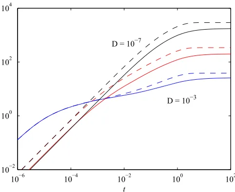
Figure1shows the results forE when starting with a very narrow peak (D0=10−8) that is very far from the origin
(y0=0.7). D=10−3, 10−5, and 10−7, and the two cases
linear and cubic are considered. Starting with the behavior for small times (t 10−4), called stage (i), there are two features
that stand out. First, the twoD=10−3 cases are far above
D=10−5and 10−7, and linear and cubic are the same. Second,
forD=10−5and 10−7, the two differentDvalues follow the
same curves, but the linear and cubic cases are now different, with linear being approximately four times greater than cubic. Also, at least for these early times, these four curves are all essentially independent oft.
To understand these results, we recall thatE is a measure of (∂p∂t)2, which in turn consists of two parts, the movement
of the PDF (advection) by the damping forceF(x) and the change in width of the PDF due to diffusionD > D0. Since
F is different in the linear and cubic processes whileDis the same,Ewould evolve similarly for both processes if dominated by diffusion (diffusion-dominated) while evolving differently if dominated by advection (advection-dominated) due to the damping force. We need to combine this knowledge with the fact that the initial evolution ofEin stage (i) is dominated for smallDby advection while for largeDby diffusion. To show this in the linear case, we examine Eq. (20) att =0:
E=2γ2
D D0 −
1 2
+γ3y02
D0
, (33)
where the first and second terms represent the effect of the diffusion and advection, respectively. Inserting γ =1, D0=10−8 and y
0=0.7, D=10−3 yields E=2×10¹⁰,
whereas D=10−5 and 10−7 both yield E=5×10⁷, as in Fig.1. Thus, in stage (i),Eexhibits the transition from diffusion dominated to advection dominated asD is reduced. Similar conclusion can be obtained for the cubic case by replacing in Eq. (33) byγe∼ζ μx 2 [Eq. (30)]. The transition point,
where the two terms in Eq. (33) are comparable, occurs when D∼y0
√
D0/2=5×10−5.
This predicted transition from advection dominated to dif-fusion dominated occurring aroundD∼y0
√
D0/2=5×10−5
is indeed observed in Fig. 1. Specifically, for D=10−3,E
is dominated by diffusion and takes the same (large) value for linear and cubic. In contrast, for D=10−5 and 10−7, E is dominated by the advection, and different evolutions are observed in linear and cubic processes. We can even understand why the linear curves are above the cubic curves by this factor of 4: If the positions of the peaks are expected to evolve asy0e−tandy0/
√
1+2y02t in the two cases (setting γ =μ=1 in the general formulas), then the speeds at which they initially move arey0 andy30, respectively (obtained by
evaluating|dtdx |att=0 in the two cases). Fory0=0.7 the
linear peak thus moves roughly twice as fast as the cubic peak, hence a factor of 4 in E. Finally, the reason these curves remain independent of time up tot ≈10−4is that the speeds of the peaks are essentially unchanged up to that time with constantF(x)∼ −γ x0 and−μx30 for linear and cubic,
respectively; diffusion is also not yet playing an important role andβ(t)=β0.
For the linear case, for somewhat larger times in stage (ii), up tot < O(1),Eexhibits a power-law decrease in time. This can also be inferred from Eq. (20) by keeping the first-order correctionT ∼γ[DD
02γ t+1]∼γ[
D
D02γ t] for
D0
2γ D t 1
(recallDD0):
E∼2γ2
1 2t2 +
y02 Dt
[image:5.608.311.557.116.205.2]
. (34)
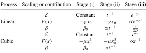
TABLE I. Scalings ofEin stages (i), (ii), and (iii) for advection-dominated case for sufficiently smallD < y0
D0
2 (D0=10− 8) and physical origins of such scaling behavior [F(x) andβ(t)]; 3< n <4. Process Scaling or contribution Stage (i) Stage (ii) Stage (iii)
E Constant t−1 e−γ t
Linear F(x) −γ x0 −γ x0 ∝e−γ t
β β0 ∝t−1 2Dγ
E Constant t−1 t−n
Cubic F(x) −μx3
0 −μx03 ∝t−1
β β0 ∝t−1 —
The second term in Eq. (34) is due to the peak with the variance
(x− x )2 ∝ =1/2β ∝t[see Eq. (17)] andF(x)= −γ x∼ −γ y0fort < O(1), which givesE ∝t−1. In comparison, the
final stage (iii) is due to the adjustment to the stationary PDF. This involves an exponential decrease inEsince
T ∼γ De
2γ t
D0
T2
ast → ∞, and thus
E =2γ2
T2 (r
2+qT)∼ 2γ2q
T ∝
1 T ∝e
−2γ t →
0,
exponentially decreasing in time ast → ∞. This is physically due to the exponential decrease in peak positiony =y0e−γ t
while β∼ γ
2D. This last stage occurs around t ≈O(1),
independent ofD.
To summarize the O-U process, for a sufficiently small D < y0
D0
2 , the relaxation of the O-U process undergoes three
scaling regimes ofEwitht: (i) constant, (ii) power law, and (iii) exponential. The stage (i) is due to the movement of the PDF; the stage (ii) is due to the diffusion with 1/β∝ (x− x )2
[see Eq. (17)] (e.g., due to the Brownian motion where the rms displacement increases ast1/2); the stage (iii) is due to the
exponential adjustment of the peak position asy=y0e−γ tin
settling into the equilibrium PDF. These scalings and leading contribution from F(x) andβ responsible for such scalings are summarized in TableI.
Sinceτ =E−1/2is the time unit or correlation time (over
which the physical time is to be measured), our results imply three stages of (i) constant, (ii) power law, and (iii) exponential scalings of the time unitτ. Furthermore, in the O-U process, the final stage starts att=O(1), the same for allD, suggesting the independence of the relaxation time on D. Alternately, this can be viewed as the independence ofx andt in linear processes sinceDonly affectsx (dependence of PDFs).
Compared to the O-U process, the time evolution ofEfor the cubic process occurs over a much longer time scale, as seen in Fig. 1. This is due to the fact that with a cubic nonlinear damping, the equilibration of a PDF to the final equilibrium quartic exponential PDF requires the timet tcwhere [31]
tc∼
1
Dμ. (35)
Astc∝D−1/2, the relaxation time becomes longer for smaller
evolution of E(t), it is useful to utilize the effective γe in
Eq. (30). Specifically, at small and intermediate times,γeis
almost independent oft as γe∝μy02, and thus the behavior
of E for the cubic process is quite similar to that of the O-U process. For stage (iii), the prediction based on Eq. (20) becomes questionable due to large fluctuations. It suffices for the purpose of this paper to conclude from Fig.1thatEin stage (iii) follows power law asE∝t−n(3< n <4). To summarize,
for a sufficiently smallD, the relaxation of the cubic process undergoes three scaling regimes ofE witht: (i) constant, (ii) power law, and (iii) power law. The stage (i) is due to the movement of the PDF, similarly to linear case; the stage (ii) is due to the diffusion, similar to the linear case. The last stage with the power-law scaling is different from the exponential scalings in the O-U process. The scalings are summarized in TableItogether with leading behavior ofF(x) andβ.
Our results demonstrate that nonlinear interaction promotes power-law scalings of statistical measuresE(τ) with respect to time. Making an analogy to power-law scaling often observed in self-organizing system which ensures scale invariance, we speculate that power-law scale of statistical measures may also be induced in self-organizing systems through nonlinear interaction. This issue will need to be explored further in the future. Furthermore, compared with the O-U process, nonlinear interaction in the cubic process results inE which varies much less rapidly. (That is to say, a power law evolves much slower than exponential.) Recalling that a geodesic is a particular path with a constantE along the path [26] which minimizes the totalLbetween given two times, we infer that the cubic process follows a path which is closer to a geodesic compared to the O-U process. Thus, we expect a smallerLin the cubic process than in the O-U process, and this will shortly be shown to be observed in our numerical results.
Furthermore, in comparison with the linear case where the relaxation time to the equilibrium is independent ofD, the dependence oftc in Eq. (35) onDreflects that the diffusion
affects not onlyx, but also key transition time scale [e.g.,tc
[image:6.608.49.290.529.727.2]in Eq. (35)], implying a close link betweenx andt through
FIG. 2. Las functions of timetfor the linear (dashed lines) and cubic (solid lines) processes. All parameter values as in Fig.1.
nonlinear interaction. We note that [31] showed that the cubic system can be linearized by introducing a nonlinear time which depends onx, which is most likely whytcis affected byD
(i.e., throughxwhich depends onD).
Finally, Fig.2showsLfor the six cases corresponding to Fig.1. SinceEin Fig.1monotonically decreases in time, the largest contribution toLcomes fromEat small times. The most prominent difference between the O-U and cubic processes is that the relaxation time tc to converge to the stationary
state is much longer for the cubic process and depends on D. Furthermore,Ltends to be smaller for the cubic process, confirming our expectation above.
VII. ATTRACTOR STRUCTURE:LVS y0
In the absence of a stochastic forcing, a system with either linear or cubic damping has one stable equilibrium point x =0, to which all initial positions approach in the long time limit. The proximity of different x to the equilibrium point x =0 can be quantified by the difference in the potential V(x) (= γ2x2 and μ
4x4 for the linear and cubic processes,
respectively), or its gradient F(x). In the presence of the stochastic forcing ξ, any initial value of x always tends to approach x=0 for sufficiently large time, and fluctuates around it, forming an equilibrium distribution. In this case, V(x) from the deterministic force does not provide an accurate measure of the difference between different initial points due toξ.
Motivated by this, [23] considered the relaxation of an initial nonequilibrium state strongly localized aroundx =y0
[i.e., modeled by p(x,0)∝δ(x−y0)] into the final
equilib-rium state around x=0 and defined the distance between the point y0 and x =0 by the total L between the initial localized PDF and the final equilibrium PDF. ThisLprovides a metric which quantifies the distance between x=y0 and
the equilibrium, serving as a useful measure to differentiate differentx’s in view of the proximity to the equilibrium point x =0.1 AsL measures different states along a path that a
system passes through, it can be viewed as a “Lagrangian or dynamic” measure of a metric. In general, when an initial PDF has a finite width [24–26], the totalLbetween an initial PDF with the mean valuey0and final equilibrium PDF was used
as the distance between y0 (mean value of x att =0) and x =0 (mean value ofx att → ∞). This metric consequently depends on both the strengthDof the stochastic noise (which determines the width of the final equilibrium PDF) and the width of the initial PDF.
In order to elucidate the effect of nonlinear interaction on the geometric structure, we now present how this metric depends ony0for differentDandD0 for the O-U and cubic
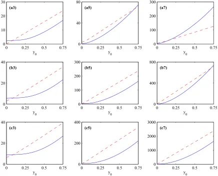
processes. Figure3shows the results of the totalL(in the limit t → ∞) as a function ofy0, forD0andDequal to 10−3, 10−5,
and 10−7. Focusing on the linear case first, the dependence
ony0 is clearly linear, except for small regions neary0=0, where a sufficiently large mismatch betweenDandD0yields results dominated by diffusion rather than movement of the
1The difference between different initial points (y
FIG. 3. Las functions ofy0for the linear (dashed lines) and cubic (solid lines) processes. The nine panels (a3)–(c7) are labeled such that rows (a,b,c) correspond toD0=10−3, 10−5, and 10−7, respectively, and columns (3,5,7) correspond toD=10−3, 10−5, and 10−7respectively. peak fromy0 to 0. TableII summarizes the slopes of these
straight lines (including also additionalDandD0values). For the simplestD=D0cases, where Fig.3indicates an exactly
linear relationship for ally0, the slopes clearly scale asD−
1 2. Above the diagonal in Fig.3 or TableII(D < D0) yields a
greater slope than below the diagonal (D > D0).
To understand these results, we examine Eqs. (22), (23), and (28). Wheny0=0, Eqs. (22) and (23) imply that L in
general has a complex dependence ony0,D0, andD. Some
simple scaling relations are, however, obtained whenD=D0,
[image:7.608.48.294.660.752.2]or wheny0is sufficiently large. First, whenD=D0,r =0; so usingTi =γ andTf → ∞(sincetf → ∞),q =β0γ y20 and
TABLE II. Slopes of L versus y0 for the linear process, for differentDandD0as indicated.
HH HHH
D0 D
10−3 10−4 10−5 10−6 10−7
10−3 31.6 60.5 95.0 131 167
10−4 41.5 100 192 301 415
10−5 46.1 132 316 606 951
10−6 47.3 148 416 1000 1917
10−7 47.5 153 467 1317 3162
2β0=γ /D0in Eq. (28) gives us
L=
2q
γ =
√γ y 0 √
D0
. (36)
Thus, when D=D0,Lhas an exact linear scaling with y0,
with slope
γ
D, as seen also in TableII(whereγ =1).
Second, for a sufficiently largey0such thatq 1, a clear linear relation betweenL andy0 is obtained, with different
slopes forD > D0 andD < D0. When D > D0 andq1
(0< r < q), the leading order contribution toLcomes from Hin Eq. (23) as (see AppendixFfor details)
tan−1
Y
qr−r2
Yf
Yi
∼ π
2 − 1
√
r0
,
wherer0= DD0 −1 and, thus (see again AppendixF),
L∼
π 2 −
D0
D
√γ y 0 √
D−D0 ∼
π
2 −
D0 D
√γ y 0 √
D , (37)
wherer∼ DD
0 is used forDD0. Thus, whenD > D0,Lis determined by measuring the change in the mean positiony0
in units of√Dto leading order, and takes its maximum value
π√γ 2
y0
√
D for a very narrow initial distribution (as D0
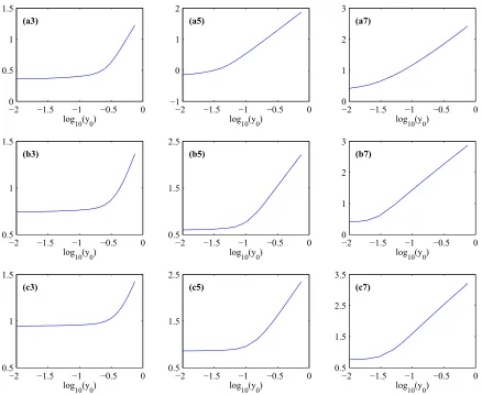
FIG. 4. As in Fig.3, but now showing log10(L) as functions of log10(y0), and for the cubic process only. These scalings can also be confirmed above the diagonals in
TableII.
When D < D0 and q 1 (r <0), the leading order
contribution toLcomes fromH in Eq. (23) as
ln
Y −r2−rq
Y +r2−rq
Yf
Yi
∼ln 2
1−√|r0|
∼ln4D0 D ,
where|r0| =1− D
D0 and, thus,
L∼ √γ y
0
2√D0
ln4D0
D ∼
ln 2+ln
D0
D √
γ y0 √
D0
. (38)
Thus, whenD0> D,Lis given byy0 measured in units of √
D0/ln
D
D0, increasing as
D0
D → ∞. It is interesting to see
the logarithmic correction factor ln
D0
D to y0 measured in
units of √D0, which is due to the narrowing of the PDF.
Again, these values are quite close to the exact results in Table
II. We have checked similar results withL∝y0for different initial PDFs (quartic exponential PDFs).
In sharp contrast to the linear case, Fig.3shows that for the cubic case, L is clearly not linearly dependent on y0.
However, plotting the same data on a log-log scale, Fig. 4
shows that for sufficiently largey0, clear power-law scalings emerge. Fory0< O(D1/4)Lis dominated by diffusion, and
hence largely independent ofy0. Fory0> O(D1/4), though, in
the regime dominated by the advection by damping forceF, all nine panels exhibit power-law behavior. For sufficiently small values of D, the power-law regime O(D1/4)< y
0< O(1)
would also extend over arbitrarily many orders of magnitude. The slopes, that is, the power-law exponents, of these straight line portions at largey0 are presented in TableIII. We infer asymptotic scalings L∼(y0)m with the exponent maround
1.5 to 1.9. This suggests that geometry is curved by the nonlinear interaction in the statistical space. What is more interesting is that this scaling ofL∝ym
0 has no resemblance
to either the quartic potential V(x)∝x4 or its gradient
F ∝x3. That is, the combined action of the deterministic force and stochastic force results in a unique characteristic
TABLE III. Slopes of log10Lversus log10y0for the cubic process, for differentDandD0as indicated.
HH HHH
D0 D
10−3 10−4 10−5 10−6 10−7
10−3 1.69 1.62 1.56 1.53 1.60
10−4 1.77 1.74 1.64 1.58 1.56
10−5 1.74 1.85 1.76 1.70 1.59
10−6 1.63 1.91 1.88 1.80 1.66
[image:8.608.312.556.658.753.2]of the geometry of the attractor, governed by a power law with indexm=m(D,D0)<2. In comparison,L∝y0for the O-U
process manifests the preservation of a linear geometry both by the linear damping force and the white-noise stochastic force.
To trace the origin of this power-law scaling, we again utilize the result that the dominant contribution toL comes from the initial and intermediate stages, where the effect of damping can be approximated by a linear friction constantγe
in Eq. (30). Thus, we can get an estimate on the upper bound onmby replacing γ byγein Eqs. (22) and (23) and taking x ∼y0as follows:
L∼
⎧ ⎨ ⎩ ψ
√μ √
Dy 2
0 ifD > D0, 0< r < q,
φ√√μ D0y
2
0 ifD < D0, r <0,
(39)
forq 1. Here,ψandφareO(1) constants. Equations (39) thus show that the power-law scaling has the upper bound as L∼ym
0 where m2. We have checked similar power
scalings for different initial PDFs (quartic exponential PDFs).
VIII. CONCLUSION
We investigated the effect of nonlinear interaction on a met-ric structure in a nonequilibrium process. By considering linear and nonlinear (cubic) damping, we computed the information change in the relaxation of an initial nonequilibrium state to a final equilibrium state and measured by the information length Lthe number of distinguishable states that a system undergoes during the relaxation. We explored scalings of statistical quantities ofτ(the inverse of the rate of change ofL) andL. Specifically, we illustrated that nonlinear interactions promoted temporal power-law scaling ofτ ∝tn. By varying
D0andD, we also demonstrated power-law scalings ofLwith
the mean positiony0of the initial PDF. For a linear damping,
an underlying linear geometry was captured in L∝y0. In
comparison, the cubic damping supports a power-law relation L∝ym
0, with a varying power indexm∼1.5–1.9, depending
onD and D0. This has to be contrasted withm=1 in the linear case. This demonstrates that nonlinear interaction tends to change geometric structure of a nonequilibrium process from linear to power-law scalings.
We emphasize thatL is path specific and is a dynamical measure of the metric, capturing the actual statistical change that occurs during time evolution. This path specificity would be crucial when it is desirable to control certain quantities according to the state of the system (e.g., time-dependent PDF) at any given time. An interesting example would be the treatment of large population (e.g., of bacteria, tumor cells) where the treatment should be adjusted according to the status of the population to optimize desirable outcomes while avoiding undesirable side effects (e.g., resistance). A toy optimization problem was addressed in terms of a geodesic solution in [26]. Due to the generality of our methodol-ogy, we envision a large scope for further applications to natural phenomena to characterize nonequilibrium processes (e.g., relaxation processes). Beyond analytical and numerically solvable models, L can be applied to any data as long as time-dependent PDFs can be constructed from data (e.g., see [24]). Such application of L to data is currently underway. Exploration of different metrics would also be of great interest.
APPENDIX A: FLUCTUATING HAMILTONIANE To appreciate the relation betweenEand fluctuating energy, we express the PDFp(x,t) as
p(x,t)=
β πe
−SA ≡e−SA+F. (A1)
Here,F= 12lnπβ is the free energy;SAis the effective action
which can be related to the HamiltonianH of the stochastic system (see [33]) as
H = −∂SA
∂t , (A2)
which is a stochastic analogy to the Hamilton-Jacobi relation [33,34]. Specifically, it was shown in [33] by a path integral formulation thatHis given in terms of
H(t)= −∂SA ∂t =
D 2
2−μx,
whereis the conjugate momentum. Note thatstems from the stochastic noise. Taking the time derivative of Eq. (A1) gives us
∂p(x,t)
∂t =( ˙F+H)p(x,t), (A3)
where ˙F= dF
dt. First, we integrate both sides of Eq. (A3) over
xand use the conservation of the total probability as follows:
0=
dx∂p ∂t =
dx( ˙F+H)p(x,t)=F˙ + H , (A4)
where H is the mean (average) value of the Hamiltonian. Therefore,
˙
F= −H . (A5)
That is, the mean value of the Hamiltonian compensates for the change in free energy to conserve the total probability. We now compute the second moment which is related toEin Eq. (20) as
E=
dx1
p
∂p ∂t
2 =
dx(H+F˙)2p(x,t)
= (H+F˙)2 = (δH)2 , (A6)
where δH=H− H =H+F˙ is the fluctuating Hamilto-nian. By using Eq. (A5), it is interesting to observe that
(δH)2 = H2 +2H F˙ +F˙2= H2 − H 2.
APPENDIX B: PHYSICAL MEANING OFL In this appendix, we make an analogy to a deterministic system to elucidate the key concepts ofτandLin Eqs. (1) and (8). Specifically, we consider the case where an object is not moving but its length changes according to the time-dependent functionl(t). For this deterministic functionl(t), the easiest way of extracting the characteristic time scaleτ(t) ofl(t) is by computing
1 τ(t) =
1 l
dl dt
By using Eq. (B1) in Eq. (8), we can then measure the total time between initialt =0 and final timetin unit ofτ(t) as
L(t)= t
0
dt1
τ(t1). (B2)
For example, if we takel(t)=Aeλt whereA >0 andλ >0
are constant, thenτ(t)=λ−1, thus, Eq. (B2) gives
L(t)= t
0
dt1 τ(t1) =
t
0
dt1λ=λt =ln
Aeλt A =ln
l(t) l(0)
.
(B3)
We realize that ll(0)(t) in Eq. (B3) is just the total number of a segment of (initial) length l(0) within the final length l(t) and that Eq. (B3) is nothing more than the entropy (by usingkB=1). Thus,L(t) characterizes the change in entropy
(amount of disorder) over timetwhen the object has no mean motion.
Switching back to the stochastic case with the time-dependent PDF p(x,t), we now consider the rate at which p(x,t) changes in time to extract the time scale ofp(x,t) as
1 τ(x,t) =
1 p(x,t)
∂p(x,t)
∂t . (B4)
As can clearly be seen from Eq. (9), the characteristic time scale τ(x,t) depends not only on t, but also x. To obtain the dynamic time unit τ(t) independent of x, we can take an average of Eq. (B4) overx as
1 τ(t) ≡
dx p(x,t) 1 τ(x,t) =
dx p(x,t) 1 p(x,t)
∂p(x,t) ∂t
=
dx∂p(x,t)
∂t =0, (B5)
where the last equality follows from the total probability conservation. Therefore, in order to obtain a nonzero τ(t), we can consider squaring Eq. (B4) before taking the average overx:
1 [τ(t)]2 ≡
dx p(x,t) 1 [τ(x,t)]2
=
dx p(x,t) 1 p(x,t)2
∂p(x,t)
∂t 2
=
dx 1 p(x,t)
∂p(x,t)
∂t 2
, (B6)
obtaining Eq. (1) in the main text. We note that Eq. (B6) corresponds to the second time derivative of relative entropy (or Kullback-Leibler divergence), as shown in Eq. (7).
APPENDIX C: COMPARISON BETWEEN LIN EQ. (26) [(27)] AND ENTROPY
To demonstrate that L take the form different from the relative entropy, it is valuable to considerp1=p(x,t1) and p2=p(x,t2) that have the same zero mean value but different
width with inverse temperaturesβ1andβ2:
p1=
β1
πe
−β1x2, p
2=
β2
πe
−β2x2. (C1)
We can then easily compute the relative entropy betweenp1
andp2as
D(p1,p2)=
dx p2ln (p2/p1)
=
dx p2ln (p2)−
dx p2ln (p1)
=
dx p2
ln
β2
π −β2x
2
−
dx p2
ln
β1
π −β1x
2
=ln
β2
π −β2x
2 2− ln β1
π +β1x
2 2 = 1 2ln β2 β1 −
1 2
1−β1 β2
. (C2)
Here,x2 2=
dx p2x2= 21β2was used. While the first term in Eq. (C2) appears to be similar to Eqs. (26) or (27), the second term inside the square brackets takes a different form. We can now show that the integral of the square root of Eq. (C2) for small |t2−t1|becomes similar to Eqs. (26) or (27). To this end, we expand terms in Eq. (C2) by lettingβ2=β1+δ:
D(p1,p2)=
1 2ln
1+ δ
β1
−1
2
1− β1 β1+δ
=1 2 δ β1 −1 2 δ2 β2 1 −1 2 δ β1
− δ2
β2 1 +O δ3
β13 =1 4 δ2 β2 1 +O δ3 β3 1 , (C3)
where ln (1+x)=x−1
2x
2+O(x3) was used. By taking a
square root of Eq. (C3), writingδ=β˙1dt, and then summing
over time in the limitδt→0, we obtain t 0 dt1 2 ˙ β1
β1 = 1 2ln
β(t)
β(0), (C4)
which is the same as the entropy change in Eq. (27).
APPENDIX D: DERIVATION OF EQ. (20) Fromp(x,t) in Eq. (13), we obtain
∂p ∂t = ˙ β 1
2β −(x−y)
2
+2β(x−y) ˙y
p, (D1)
where we recally = x =y0e−γ t. Using Eq. (D1) in Eq. (1)
gives us
1 [τ(t)]2 =
dx
1
2β −(x−y)
2
˙
β+2β(x−y) ˙y 2
p
=β˙2
1 2β
2
− 1
β(x−y)
2 + (x−y)4
+4β2(x−y)2 y˙2
= 1
2β(t)2
dβ dt
2 +2β
dy dt
2
Here, ˙β= dβdt and ˙y = dydt; we used (x−y)2 = 1
2β and
(x−y)4 =3(1 2β)
2
. To obtain the last equation in Eq. (20), it is useful to expressβ in Eq. (18) in the following form:
β = 1
1 β1 +
1 β0e
−2γ t =
1
2D(1−e−2γ t)
γ +
1 β0e
−2γ t (D3)
= γ β0e2γ t
T , (D4)
where we usedT =2β0D(e2γ t−1)+γ. By differentiating
Eq. (D3), we then obtain
˙
β = −2γ β2e−2γ t 2D γ − 1 β0
= −2β2e−2γ t[2β0D−γ]
1 β0
. (D5)
Equations (D4) and (D5) andr=2β0D−γ then give us
˙ β2 2β2 =2γ
2r2 1
T2. (D6)
Similarly, using y˙= dtd(y0e−γ t)= −γ y0e−γ t, T =
2β0D(e2γ t−1)+γ, andq=β0γ y02, we obtain
2βy˙2 =2qγ21
T. (D7)
Finally, using Eqs. (D6) and (D7) in Eq. (D2) gives us Eq. (20).
APPENDIX E: DERIVATION OF EQS. (22) AND (23) By using Eqs. (20) and (21) in Eq. (8), we obtain
L=√1
2 Tf Ti 1 T 1 T +r
r2+qT
dT . (E1)
To compute Eq. (E1), we letY =r2+qT and recast it as
L= √ 2 r Yf Yi r2 Y2−r2 +
qr−r2 Y2+qr−r2
dY
=√1
2
ln
Y −r
Y +r Yf
Yi
+ √
2
r H, (E2)
whereYiandYfareYevaluated atTiandTf, andHis defined
as
H= Yf
Yi
qr−r2
Y2+qr−r2dY. (E3)
Equation (E3) is to be evaluated separately for two cases: qrandq < r. First, forq r, we useY =qr−r2tanθ
in Eq. (E3) to obtain
H =qr−r2
sec2θ
tan2θ+1dθ (E4)
=qr−r2
tan−1
Y
qr−r2
Yf
Yi
. (E5)
Second, in the q < r case, we let Y =|qr−r2|secθ=
r2−qrsecθ(cosθ= √
r2−qr
Y ) to obtain
H = −r2−qr
1 sinθdθ
= −
r2−qr
2
ln
Y−r2−qr
Y+r2−qr
Yf
Yi
. (E6)
We note that Eq. (E2) is continuous acrossq=r. In summary, Eqs. (E5) and (E6) lead to Eq. (23) in the text; Eq. (E2) gives Eq. (22) in the text.
APPENDIX F: DERIVATION OF EQ. (37)
In this appendix, we show the main steps leading to Eq. (37) whenD > D0,q 1, and 0< r < q. In this case, we note
thatHin Eq. (22) is given by the first line in Eq. (23) and thus
H r =
q
r −1 tan
−1
Y
qr−r2
, (F1)
where
Y =qT +r2, q =γ 2y2
0
2D0
, r=γ D D0 −1 ,
T =γ
D D0(e
2γ t−
1)+1
.
We evaluate Eq. (F1) at t =0 and t→ ∞ to compute the second term on the right-hand side of Eq. (22). To this end, first, we approximate the argument of the arctan function in Eq. (F1) for largeq 1 as
Y
qr−r2 =
qT r2 +1
q r −1
∼ T r ∼ D0
D−D0
D
D0
(e2γ t−1)+1
. (F2)
In the long time limit as t→ ∞, we let φ≡ D0
D−D0 [DD
0(e
2γ t−1)] (→ ∞), and evaluate Eq. (F2) as
Y
qr−r2
t→∞ ∼
φ+ D0
D−D0. (F3)
On the other hand, att=0, Eq. (F2) is simplified as
Y
qr−r2
t=0 ∼
D0
D−D0. (F4)
We now evaluate
q
r −1 in front of the arctan function in
Eq. (F1) att =0 andt → ∞, which in both limits becomes
q r −1∼
γ y02
2D −1∼
γ
Thus, by putting Eqs. (F3)–(F5) in Eq. (F1), we obtain
H
r ∞
t=0 ∼y0
γ 2D
tan−1
φ+ D0 D−D0
−tan−1
D0
D−D0
∼y0
γ 2D
π
2 −
D0
D
, (F6)
by using φ→ ∞, D0D, and tan−1x∼x for x 1.
In comparison with the contribution from the second term involvingHon the right-hand side of Eq. (22), the contribution from the first term involving the logarithmic function can be shown to be negligible by following similar analysis as above. Therefore, multiplying Eq. (F6) by√2 gives Eq. (37) in the main text.
[1] H. Haken,Information and Self-Organization: A Macroscopic Approach to Complex Systems(Springer, Berlin, 2006). [2] W. B. Cannon, Organization for physiological homeostasis,
Physiol. Rev.9, 399 (1929).
[3] E. Kim and P. H. Diamond, Zonal Flows and Transient Dynamics of the L-H Transition,Phys. Rev. Lett.90,185006(2003). [4] K. Srinivasan and W. R. Young, Zonostrophic instability,
J. Atmos. Sci.69,1633(2006).
[5] A. L. Gibbs and F. E. Su, On choosing and bounding probability metrics,Int. Stat. Rev.70,419(2002).
[6] R. Jordan, D. Kinderlehrer, and F. Otto, The variational formulation of the Fokker-Planck equation,SIAM J. Math. Anal.
29,1(1998).
[7] A. Takatsu, Wasserstein geometry of Gaussian measures, Osaka J. Math.48, 1005 (2011).
[8] J. Lott, Some geometric calculations on Wasserstein space,
Commun. Math. Phys.277,423(2008).
[9] W. Gangbo and R. J. McCann, The geometry of optimal transportation,Acta Math.177,113(1996).
[10] S. Ferradans, G.-S. Xia, G. Peyr´e, and J.-F. Aujol, Static and dynamic texture mixing using optimal transport,Lecture Notes Comput. Sci.7893,137(2013).
[11] H. Risken,The Fokker-Planck Equation: Methods of Solutions and Applications(Springer, Berlin, 2013).
[12] W. K. Wootters, Statistical distance and Hilbert space,
Phys. Rev. D23,357(1981).
[13] M. T. Martin, A. Plastron, and O. A. Ross, Statistical complexity and disequilibrium,Phys. Lett. A311,126(2003).
[14] G. Ruppeiner, Thermodynamics: A Riemannian geometric model,Phys. Rev. A20,1608(1979).
[15] F. Schl¨ogl, Thermodynamic metric and stochastic measures,
Z. Phys. B: Condens. Matter59,449(1985).
[16] E. H. Feng and G. E. Crooks, Far-from-equilibrium measure-ments of thermodynamic length, Phys. Rev. E 79, 012104
(2009).
[17] S. L. Braunstein and C. M. Caves, Statistical Distance and the Geometry of Quantum States,Phys. Rev. Lett.72,3439(1994). [18] H. Strobel, W. Muessel, D. Linnemann, T. Zibold, D. B. Hume, L. Pezz´e, A. Smerzi, and M. K. Oberthaler, Fisher information and entanglement of non-Gaussian spin states,Science345,424
(2014).
[19] J. Nulton, P. Salamon, B. Andresen, and Q. Anmin, Quasistatic processes as step equilibrations,J. Chem. Phys.83,334(1985).
[20] G. E. Crooks, Measuring Thermodynamic Length,Phys. Rev. Lett.99,100602(2007).
[21] D. A. Sivak and G. E. Crooks, Thermodynamic Metrics and Optimal Paths,Phys. Rev. Lett.108,190602(2012).
[22] P. Salamon, J. D. Nulton, G. Siragusa, A. Limon, D. Bedeaux, and S. Kjelstrup, A simple example of control to mini-mize entropy production,J. Non-Equilib. Thermodyn.27,45
(2002).
[23] S. B. Nicholson and E. Kim, Investigation of the statistical distance to reach stationary distributions,Phys. Lett. A379,
83(2015).
[24] S. B. Nicholson and E. Kim, Structures in sound: Analysis of classical music using the information length,Entropy18,258
(2016).
[25] J. Heseltine and E. Kim, Novel mapping in non-equilibrium stochastic processes, J. Phys. A: Math. Theor. 49, 175002
(2016).
[26] E. Kim, U. Lee, J. Heseltine, and R. Hollerbach, Geometric structure and geodesic in a solvable model of nonequilibrium process,Phys. Rev. E93,062127(2016).
[27] E. Kim, H.-L. Liu, and J. Anderson, Probability distribution function for self-organization of shear flows,Phys. Plasmas16,
052304(2009).
[28] A. P. L. Newton, E. Kim, and H.-L. Liu, On the self-organizing process of large scale shear flows,Phys. Plasmas20,092306
(2013).
[29] E. T. Lu, Avalanches in Continuum Driven Dissipative Systems,
Phys. Rev. Lett.74,2511(1995).
[30] M. H. Pinsonneault, S. D. Kawaler, S. Sofia, and P. Demarque, Evolutionary models of the rotating Sun,Astrophys. J.338,424
(1998).
[31] E. Kim and R. Hollerbach, Time-dependent probability density function in cubic stochastic processes,Phys. Rev. E94,052118
(2016).
[32] F. Klebaner,Introduction to Stochastic Calculus with Applica-tions(Imperial College Press, London, 2016).
[33] E. Kim and S. Nicholson, Complementary relations in non-equilibrium stochastic processes, Phys. Lett. A 379, 1613
(2015).