State Aggregation through Reasoning in Answer Set Programming

This is a repository copy of State Aggregation through Reasoning in Answer Set

Programming.

White Rose Research Online URL for this paper:

http://eprints.whiterose.ac.uk/102693/

Version: Accepted Version

Conference or Workshop Item:

Gaudioso, G, Leonetti, M orcid.org/0000-0002-3831-2400 and Stone, P (2016) State

Aggregation through Reasoning in Answer Set Programming. In: IJCAI Workshop on

Autonomous Mobile Service Robots, 11 Jul 2016, New York, United States.

[email protected] https://eprints.whiterose.ac.uk/ Reuse

Unless indicated otherwise, fulltext items are protected by copyright with all rights reserved. The copyright exception in section 29 of the Copyright, Designs and Patents Act 1988 allows the making of a single copy solely for the purpose of non-commercial research or private study within the limits of fair dealing. The publisher or other rights-holder may allow further reproduction and re-use of this version - refer to the White Rose Research Online record for this item. Where records identify the publisher as the copyright holder, users can verify any specific terms of use on the publisher’s website.

Takedown

If you consider content in White Rose Research Online to be in breach of UK law, please notify us by

In Proceedings of the IJCAI Workshop on Autonomous Mobile Service Robots, New York City, NY, USA July 2016

State Aggregation through Reasoning in Answer Set Programming

Ginevra Gaudioso, Matteo Leonetti, and Peter Stone

Department of Computer Science

University of Texas at Austin

[email protected],

{

matteo,pstone

}

@cs.utexas.edu

Abstract

For service robots gathering increasing amounts of information, the ability to realize which bits are rel-evant and which are not for each task is going to be crucial. Abstraction is, indeed, a fundamental characteristic of human intelligence, while it is still a challenge for AI. Abstraction through machine learning can inevitably only work in hindsight: the agent can infer whether some information was per-tinent from experience. However, service robots are required to be functional and effective quickly, and their users often cannot let the robot explore the environment long enough. We propose a method to perform state aggregation through reasoning in an-swer set programming, which allows the robot to determine if a piece of information is irrelevant for the task at hand before taking the first action. We demonstrate our method on a simulated mobile ser-vice robot, carrying out tasks in an office environ-ment.

1

Introduction

Service robots will have to perform a variety of tasks for ex-tended periods of time, inhabiting their environment perma-nently. They are subject to continuously accumulating knowl-edge, which can quickly become overwhelming. Decision making requires robots to process such knowledge repeatedly, with the additional challenge, brought about by sharing the environment with humans, of having to do so with a respon-siveness that does not make the users impatient.

Being able to realize which pieces of information are rele-vant for which task will become an indispensable skill. This ability ofabstractingirrelevant details is a formidable char-acteristics of human intelligence, which is still a challenge for AI. A person learning the shortest path between two rooms in a building would have no problem realizing that the weather outside has no bearing on his task. He would not need to learn it from data, trying a certain path with sunshine and with rain to verify it takes the same time. He would just be able to re-alize it by reasoning. This human capability is what we want to achieve by automated reasoning.

In this paper, we propose a system which leverages auto-mated reasoning in Answer Set Programming (ASP) to

de-termine a set of possible courses of action for the robot, and the respective relevant information. Reinforcement learning is then performed to learn the best behavior for the task, learn-ing decisions that depend only on the knowledge that the ASP reasoner has deemed pertinent.

By reasoning on a model, the agent can direct the execu-tion towards the goal, without the need to explore the whole environment. Through reinforcement learning, the agent can adjust to the environment, adapting in the (very likely) case of inaccuracies of the model. By learning alone, however, the only way to realize whether some features of the perceived state are irrelevant for the optimal behavior is in hindsight: after trying the same actions multiple times, statistical tests can reveal that certain states can indeed be abstracted. In cer-tain cases as our example above, on the other hand, we expect that reasoning on a model of the environment should provide such an abstraction even before acting. For this reason, we propose a combination of automated reasoning in ASP and reinforcement learning, to benefit from both the forward view of reasoning and the backward view of learning.

2

Background

2.1

Answer Set Programming

Answer Set Programming is a form of declarative ming, based on the stable model semantics of logic program-ming [Lifschitz, 2008]. Its syntax is defined in terms of atoms,literals, andrules. An atom is an elementary propo-sition, such as por -q, while a literal is an atom with our without negation, such aspornot q. A rule is is an expres-sion of the form:

p, . . ., q :- r, . . ., s, not t, . . ., not u

The symbolnot is often referred to asnegation as failure. The classical negation of an atompis denoted with-p, and is another atom, with the constraint that ifpis in the answer set then-pcannot be in the answer set, and vice versa.

Achoicerule is a particular rule whose syntax is as follows:

{p, . . ., q} :- r, . . ., s, not t, . . ., not u If the body is verified by the answer set, then zero or any number of atoms in{p, . . . ,q}may be in the answer set. Two other special cases of rules arefactsandconstraints. Afactis a rule in which the body is missing. Aconstraintis a rule in which the head is missing. For instance, “:- q” means that qcannot belong to any answer set.

To compute the answer sets of a given program, we used the answer set solverclingo[Gebseret al., 2011].

2.2

Planning in Answer Set Programming

We want to represent a dynamical systemDm=hS,A, fmi

in Answer Set Programming. The setSis a set of states,A

is a set of actions, andfm :S × A →2S is the (potentially

non-deterministic) transition function.

The set of states is represented in terms of predicates whose truth value may change at different time steps, and that for this reason are calledfluents. Given a finite set of fluents,F, the set of states S = 2F

is the set of all possible truth as-signments (positive or negative) to the fluents inF. In ASP, however, a fluent may havethreevalues: appear in an answer set, appear negated, or not appear at all. Therefore, answer sets can be partial assignments to the fluents, where some flu-ents result unspecified. Such answer sets may correspond to more than one state (the ones obtained by assigningtrueor falseto the missing fluents in all possible ways), and we will refer to them asbelief states. LetB= 3F

be the set of belief states over the fluents inF. Letc:B →2S

be a completing function which for any belief statebreturns the set of states obtained by assigning to the fluents inF \btruth values in all possible ways. We can establish a partial ordering over belief states, determining that a belief statebismore generalthan a belief stateb′

iffc(b)⊇c(b′

), denoted withbb′

.

Actions are represented in the same way as fluents, and are syntactically indistinguishable from them. For instance, openDoor(d1,0), is an atom that means that the action openDooris executed on doord1at time step0. The tran-sition functionfmis represented in the ASP theory by

deter-mining how fluents are carried over from one time step to the next by actions, or just by the passage of time.

The pre-condition of actions is represented with con-straints. For instance:

:- openDoor(D,I), not facing(D,I)

means that it is not possible to execute actionopenDoor(D) iffacing(D)cannot be proven at time stepI.

The effect of actions is represented with rules such as: open(D,I+1):- openDoor(D,I)

which means that executing the action openDoor(D) at time stepIcauses the door to be open at time stepI+1.

A planning problem P = hDm, s0,Gi is a tuple where

Dmis a transition system,s0is the initial state, andGis a set

of states. The initial state is specified through a set of facts

about the time step0, while the goal state is specified through constraints excluding, from the possible set of states at the last time step, all the states that do not fulfill a given goal. The ASP reasoner grounds all the rules, and generates a theory up to a given time step n, whose answer sets are all and only the histories of the formhs0, a0, . . . , sn−1, an−1, sni, where

sn ∈ G. The sequence of actionsp = ha0, . . . , an−1iis a

plan that achieves a goal state inG.

2.3

Optimization in Answer Set Programming

The answer set solverclingosupports optimization state-ments, which allow the programmer to obtain not just any answer set but an optimalone. We take advantage of this feature, since we want to compute theminimumset of flu-ents necessary to estimate the cost of a plan. An optimization statement can be specified as follows:

opt { L1, ..., Ln }

whereoptcan be either#minimizeor#maximize, and the symbolsLnare literals. As a consequence of the presence

of this statement, the answer set solver will return an answer set which has either the minimum or the maximum possible number of literals specified in the statement.

Answer set programming allows us to write very compact models, and the answer set solverclingocan return not just one plan but all plans that fulfill certain constraints, which will be necessary for the definition of our method. Further-more, the ability to optimize over the answer sets allows us to define theminimumsolution as the more abstract, enabling the reasoning at the foundation of state aggregation. A draw-back of automated reasoning is that decisions originate from the model only, and any discrepancies between the environ-ment and the model may lead to a failure. We overcome this weakness through reinforcement learning, grounding de-cisions also on data from experience.

2.4

Markov Decision Processes

We introduce briefly in this section the notation we use for Markov Decision Processes, referring to one of the many more specialized texts for a complete discussion [Sutton and Barto, 1998]. We denote a Markov Decision Process as

D = hS,A, f, ri, whereS is the set of states,Ais the set of actions, f is the transition function and r is the reward function. We denote withA(s)the actions available in state

s. The behavior of the agent is represented as a function

π :S → Acalled a(stationary deterministic) policy, which returns the action to execute in each state.

A number of methods exist which return an optimal policy by computing avaluefunction:

qπ(s, a) =

X

s′

f(s, a, s′

)(r(s, a, s′

) +γq(s′ , π(s′

))), (1)

where0 < γ ≤1is thediscount factor. The value function computes the expected return for taking actionainsand fol-lowingπthereafter. A policyπ∗

isoptimaliffqπ∗(s, a) ≥

qπ(s, a), for every other policyπ, and∀s∈ S, a∈ A.

A popular function approximator, for which implementa-tions are widely available, is Tile Coding with hashing [Sut-ton and Barto, 1998]. In tile coding the state space is parti-tioned intotiles, where the union of a layer of tiles forms a tiling. A featureφi(s)∈ {0,1}corresponds to each tile, and

therefore, only one feature can return1per tiling. It is pos-sible to have multiple tilings slightly shifted from each other span the state space, or at different resolutions.

We will use Sarsa(λ) [Sutton and Barto, 1998] for control, estimating the value function with True Online TD(λ) [Seijen and Sutton, 2014]. The exploration will be anǫ-greedy strat-egy. With theǫ-greedy strategy, the agent chooses the current optimal action according toqπ with probability1−ǫ, and a

random action with probabilityǫ.

Reinforcement learning allows the agent to learn an opti-mal behavior with no prior knowledge. In practice, however, this often requires an infeasible amount of experience. This issue is addressed by DARLING, a method combining plan-ning and reinforcement learplan-ning described in the next section.

2.5

Domain Approximation for Reinforcement

Learning

The approach presented in this paper builds on a method to generate a reduced MDP for reinforcement learning through planning, called Domain Approximation for Reinforcement LearnING (DARLING). DARLING comprises three steps: plan generation, plan filtering and merging, and reinforce-ment learning.

Plan GenerationThe user is required to provide an ASP modelDm =hS,A, fmiof an MDPD =hS,A, f, ri. For

this paper we only consider MDPs that can be modeled in ASP, therefore with discrete action and state spaces. The first step consists of computing all plans of length at mostL=µ·l

wherelis the length of the shortest plans, andµ≥1is a pa-rameter of the method, which determines how suboptimal a plan can be in the model in order to be considered for rein-forcement learning in the environment.

Plan Filtering and MergingLetP be the set of the plans computed at the previous step. Some plans inP may be re-dundant, that is, they may contain a sequence of actions such that, if removed from the plan, what remains is also a plan. For instance, a plan containing a cycle is redundant. If a plan is not redundant it is said to beminimal. Redundant plans are filtered out ofP, and the remaining plans form the setΠ(L) of all the minimal plans of length at mostL. The plans that belong toΠ(L)are then merged into apartialpolicy

πL(s) ={a|∃p∈Π(L) s.t.hs, ai ∈p}, ∀s∈ S. (2)

While a policy is a function that returns an action for each state of an MDP, a partial policy is a functionπ : S → 2A

which returns the set of all the actions that belong to at least one plan. Such a function is used in the last step of DAR-LING to define a reduced MDPDr on which the agent can

do reinforcement learning.

Reinforcement Learning and ExecutionAt run time, the agent can choose only among the actions returned by the partial policy, and it estimates their value by reinforcement learning to make an informed choice. The partial policy re-duces the MDP in which the agent effectively learns from

D = hS,A, f, ritoDr = hS,Ar, fr, ri, where the actions

available are restricted to those returned by the partial policy:

Ar(s) =πL(s). The transition function is defined from the

one ofD: fr(s, a, s′) =f(s, a, s′), ∀s, s′ ∈ S, a∈ Ar(s),

but it is undefined for actionsa /∈ Ar(s).

If the agent finds itself in a state for whichπLreturns no

ac-tion, it can replan from that state, compute a new partial pol-icy, and merge it with the current one, augmenting the MDP in which it learns.

3

Related Work

Li et al. [Liet al., 2006] identify several levels of abstrac-tion for Markov Decision Processes, from the strictest, cor-responding to Bisimulation [Givan et al., 2003], in which two states are aggregated only if the full one-step model corresponds exactly, to Policy Irrelevance [Jong and Stone, 2005], in which only the optimal action has to be maintained when merging two states. Our method is at an intermedi-ate level, indicintermedi-ated by Li et al. as Q∗

-Irrelevance, since it aims at preserving the optimal value function. At the same level of abstraction are the G-algorithm [Chapman and Kael-bling, 1991], and stochastic dynamic programming with fac-tored representation [Boutilieret al., 2000]. The former ini-tially collapses every state, and later performs statistical tests to split particular states when necessary. It is a learning al-gorithm, which does not require a model of the MDP, but does require experience to gather enough data for the sta-tistical tests. Conversely, our method is based on reasoning on a model, and no prior experience is required to determine which information is certainly irrelevant.

Factored representations allow for a natural description of many domains in terms offeatures. Stochastic dynamic pro-gramming on factored MDPs is a decision-theoretic method, and it works on a model of the MDP, like our method, but it requires an exact, stochastic, model. Our method, on the other hand, requires an ASP model of the environment, which does not include transition probabilities and actions costs. Re-lated to factored representation is Relational Reinforcement Learning (RRL) [Dˇzeroskiet al., 2001]. The aim of RRL is making use of a relational, first-order, representation to gen-eralize through logic induction. It is particularly powerful in domains that can be naturally expressed in terms of objects and relations among them. Even if generalizing through first-order lifted inference, RRL methods still calculate values and policies for the full domain, while our method uses ASP (in its propositional definition) to reduce the portion of the region to explore, and apply the generalization to that region only.

Lastly, the most common method for state aggregation for RL is through function approximation. In particular, tile cod-ing described in Section 2.4, is one of the most popular lin-ear function approximators. For this reason, we compare our method against Tile coding in Section 5.1.

4

Method

humans that certain features of the environment have no im-pact on a particular task, for instance the weather outside of a building for indoor navigation. We aim at formalizing and implementing such reasoning in ASP, so that the agent can realize that certain aspects of the environment do not matter for the task at hand, even before taking the first action.

As a motiving example, consider a service robot perform-ing tasks in the buildperform-ing shown in Figure 1. The robot

re-Figure 1: Simulation environment of an office building.

members whether the doors in front of it are open or closed. If the robot is in roomA, as shown in the figure, and it has to navigate to roomB, the state of only a few of the about30 doors on the floor actually affects the navigation.

We are interested in determining when two states are equiv-alent for the purpose of computing an optimal policy in the restricted MDPDr. If in two statessands′the same actions

are available, and each action has the same value under the optimal policy:

Ar(s)≡Ar(s

′

)∧qπ∗(s, a) =qπ∗(s

′

, a),∀a∈Ar(s) (3)

thensands′

can beaggregated, which we will denote with

B(s, s′

).

As introduced in Section 2.2, it is possible in ASP to reason in terms of belief states, that is, states in which some fluents are not assigned a truth value. Some belief states are more general than others, in that they correspond to larger sets of fully specified states.

For each statesfor which the partial policy (Eq. 2) returns a non-empty set of actions, we want to compute the most gen-eral belief stateb∗

such that the following conditions hold:

s∈c(b∗) (4)

B(s, s′)∀s, s′ ∈c(b∗) (5) ∄b. bb∗∧B(s, s′)∀s, s′ ∈c(b) (6)

that is,b∗

is the maximal equivalence class for the value func-tion containing the states. Such a belief stateb∗

would not contain any of the fluents that are irrelevant for distinguishing states for the purpose of estimating the optimal value func-tion. Therefore, it would be possible to learn the same value for all the states inc(b∗

), accelerating learning considerably. Executing DARLING, the agent has already computed Π(L). The plans are stored in a directed acyclic graph

G = hV, Ei, whereV = {s|∃p ∈ Π(L) s.t. hs, aii ∈ p}, is the set of nodes which is composed of the states that are traversed by at least one plan, and E = {hsi, ai, sji|∃p ∈

Π(L) s.t. hsi, aii,hsj, aji ∈ p∧sj = si+1} is the set of

edges, labeled by the actions, which link two states if they appear one immediately after the other in at least one plan.

We require the user to specify the one-step model for esti-mating action costs, and we take advantage of an automated reasoner to verify which bits of information are necessary.

We add an additional requirement to the specification of actions in ASP: a pre-condition for an actionais verified in a belief statebif: (1) the action is executable in any state of

c(b), and (2) the agent has all the necessary information to correctly estimate the cost ofafrom any state inc(b). The second requirement is usually not present in planning, but it will allow the reasoner, with an appropriate query, to chain the necessary knowledge for estimating action costs.

For instance, the robot of our example has an action approachDoor(D,I)to approach a doorDat time step

I. We use time as a metric for action costs. The pre-condition of such an action requires (1) the agent to be at a location con-nected to the door (to enable the action) and (2) to know the room in which the robot is, and the door it is beside. The second part of the pre-condition is necessary to be able to as-sociate a cost with the action.

In order to compute the most general current belief state, the agent generates an ASP query for each plan available from the current state. First, the current state is located in the graph

G. If not present, the agent can replan. Then, the graph is visited with a depth first search starting from the current state. For each plan, the agent constructs the following query:

1. For each fluentpi in the current state, add a choice rule {pi}.

2. Add an optimization statement with each fluentpiin the

current state:#minimize {p1, p2, ..., pi}.

3. For each actiona(C,i)with constantsCat time stepi

in the current plan, add the action as a fact:a(C,i).

4. Add the goal.

The resulting query is similar to a planning query, since it contains the goal, but the choice rule is not on the actions, which on the contrary are specified as facts, but on the fluents of the initial state. Because of the minimization statement, only the fluents that are necessary for the plan to achieve the goal will be added. Hence, this method explicitly takes ad-vantage of the fact that the agent knows what it is going to do, and can therefore reason about what information will be necessary down the road.

Consider the plan in the example that goes from room A

to room B through the doors A1 and B1. The knowledge

base of the robot could contain the state of 10 doors, still leaving about20more unspecified. It also certainly contains the fluentat(roomA,0)specifying that the robot is in room

A, and the fluentbeside(A1,0), since the robot is beside door A1. A minimization of the fluents of the current state

would leave only theatandbesidefluents, and the fluents encoding the state of doorsA1andB2. The state of any other

door would be removed from the answer set.

The query returns the minimum answer setASifor a

par-ticular planpi. The minimum belief state containing the

cur-rent state is then computed asb∗

= ∪ASi, the union of all

informa-tion. This is the most we can extract from the model, but more aggregation can be performed learning from data.

5

Experimental Validation

We validate our method to aggregate states through reasoning in ASP in two domains. The first domain is a grid world de-signed to serve as an illustration of the method. It allows us to run a large number of trials, and to compare our method with Tile Coding. The second domain is the realistic simulation of a mobile service robot introduced above.

5.1

Gridworld Domain

The grid-world domain designed to illustrate our method is represented in Figure 2. The state is composed of the agent’s

Figure 2: The Gridworld used for this experiment.

position in the grid and the grid’s color. The position is rep-resented ashx, yicoordinates, where the bottom left corner ish0,0iand the top right corner ish4,4i. The color repre-sents information which is irrelevant for navigation tasks in the grid. The agent moves by executing the actionsnorth, south,eastandwest, which deterministically move the agent in the respective direction, unless it would take the agent out of the grid, or make it hit the wall, in which case the agent does not move. In Figure 2, the wall is the thick black line. The pre-conditions of the actions require the agent to know its position, but do not require the color.

The wall has been added to illustrate the effect of DAR-LING. We ran DARLING withµ= 1, so that only the plans that are optimal in the model (shortest plans) are retained. The resulting reduced MDPDrcontains only actions to reach

the bottom cells, and the cells on the right-hand side of the wall, as shown in Figure 2. There are 15shortest plans in this grid, but only one of them is the optimal plan in practice. Since the ASP model of the environment does not contain the reward, the optimal plan will have to be learned. The reward returned for entering each cell is also shown in Figure 2.

The agent goes from the starting position (marked with S in the figure) to the goal position (marked with G) for100 episodes. The color of the grid was randomly assigned as part of the initial state out of a set of 100 colors.

We compare the agent performing state aggregation with our method against four agents that do state aggregation with tile coding, and one which learns in the full state space, with-out doing any aggregation. The agents using tile coding have as input the state vectorhx, y, ci, where the first two variables are the coordinates of the agent in the grid, andc ∈ [0,99] encodes the color of the grid. Each tile coding agent employs

a group of 8 tilings with2 ×2 cells on the first two vari-ables, and different sizes on the color variable, namely: 2, 10,50, and100. A drawback we can immediately note about state aggregation with tile coding is that the representation has to be designed by hand. The parameters of Sarsa(λ) are

α= 0.1,γ=λ= 0.9,ǫ= 0.5. For tile coding,αhas been normalized by the number of tilings.

The results, shown in Figure 3, are averaged over 1000 tri-als, and a sliding windows of 5 episodes. The plot also shows the 95%confidence intervals every5points. The agent

im-Figure 3: The results of the grid-world experiment.

plementing our method filters out the information about the color at planning time, and the input to its learning layer con-tains only the position of the agent. Even if learning with a tabular representation, it can outperform all of the tile coding agents. The performance of tile coding agents increases, as expected, with the generalization over the irrelevant variable. The agent learning in the full state space in tabular form is the slowest to learn, since it has to re-learn the optimal action for each state for every color of the grid.

In this experiment the irrelevant knowledge has been in-jected in the design of the environment, and can be identified easily. In the next domain we show a realistic scenario in which relevant and irrelevant fluents have to be determined state by state.

5.2

Robot Navigation Simulator

The second domain was introduced in Section 4 and is shown in Figure 1. The simulation is controlled by the same code that controls our robots, executed in the Robot Operating Sys-tem (ROS), while the 3D simulation was built in Gazebo1.

The state of the environment is represented by a set of flu-ents as follows. Theat(R,I) fluent represents the posi-tion of the robot; beside(D,I)andfacing(D,I) in-dicate the position of the robot with respect to doorD; the open(D,I)fluents represent the state of the doors. The set of actions is: gothrough(D,I);opendoor(D,I); approach(D,I), where D is a door, with their literal meaning. The reward function isr(s, a, s′

) = −t(s, a, s′

), wheret(s, a, s′

)is the time in seconds it took to execute ac-tionafromstos′

.

The robot had a sequence of three tasks to perform, which was repeated 500 times. Each task has the goal of reaching

(a) Task 1, action 1. (b) Task 1, action 2.

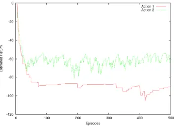
Figure 4: The estimated return without state aggregation for the initial states corresponding to the single belief state of Figure 5

Figure 5: The estimated return with state aggregation for the most frequent initial belief state.

one of the three roomsA,B, orC, starting from the preceding one in a loop.

The state of the environment changed every 5 iter-ations of the tasks: some randomly chosen doors in

{A1,A2,A3,B1,B2,B3,C1,C2}were closed and others were opened, to simulate the effect of people in the real envi-ronment. When approaching a door the robot can sense its state, and therefore update the knowledge base following the changes in the environment. The parameter wereµ= 1.5for DARLING, andα= 0.8,γ= 0.9999,λ= 0.9, andǫ= 0.15 for Sarsa.

Each simulated trial took about14hours in real time, which corresponds to 2.5 times as much simulated time. For this reason we could not run as many trials as with the grid-world domain. For this experiment, we show the impact of state ag-gregation on the estimate of the value function in the initial state, which converges to the robot’s estimate for the whole task. For each task we identified the aggregated belief state which was the most frequent initial state. Let this belief state be bi. Then we determined which states in c(bi) were the

initial state when the agent was not performing state aggrega-tion. The single most common aggregate belief state corre-sponds to11initial states for Task 1,6for Task 2, and again 11for Task 3. It means that the agent not performing state

aggregation had to learn the same values for the same ac-tions11,6, and11times respectively just for the initial state, while it only had to learn them once while doing state aggre-gation. The estimates learned for state aggregation are shown in Figure 5, while the estimates without state aggregation are shown, for each of the11states that should have been aggre-gated, in Figure 4. Note that the estimates converge for state 2, the most frequent, while for the other states they are still converging. For all these other states, using the aggregated knowledge would provide a correct estimate, while the value of those actions had to be relearned.

6

Conclusion

We propose a method to perform state aggregation based on reasoning in answer set programming. The method allows the robot to realize, before execution, what pieces of infor-mation are certainly going to be irrelevant for learning an op-timal policy. We demonstrated the approach on two domains, one of which is a realistic simulation of a service robot in an office environment. We show how much can be gained by doing state aggregation, since just in the initial state of one of the three tasks performed, the agent had to relearn the same action values11times. This learning effort could be spared if the robot realized that those 11 initial states are actually equivalent for the task at hand. This ability is going to be crucial for service robots which will deal with constantly in-creasing amounts of information.

7

Acknowledgements

References

[Boutilieret al., 2000] Craig Boutilier, Richard Dearden, and Mois´es Goldszmidt. Stochastic dynamic program-ming with factored representations. Artificial Intelligence, 121(1):49–107, 2000.

[Chapman and Kaelbling, 1991] David Chapman and Leslie Pack Kaelbling. Input generalization in delayed reinforcement learning: An algorithm and performance comparisons. In International Joint Conference on Artificial Intelligence, volume 91, pages 726–731, 1991. [Dˇzeroskiet al., 2001] Saˇso Dˇzeroski, Luc De Raedt, and

Kurt Driessens. Relational reinforcement learning. Ma-chine learning, 43(1):7–52, 2001.

[Gebseret al., 2011] Martin Gebser, Benjamin Kaufmann, Roland Kaminski, Max Ostrowski, Torsten Schaub, and Marius Schneider. Potassco: The potsdam answer set solv-ing collection.Ai Communications, 24(2):107–124, 2011. [Gelfond and Lifschitz, 1988] Michael Gelfond and Vladimir Lifschitz. The stable model semantics for logic programming. In ICLP/SLP, volume 88, pages 1070–1080, 1988.

[Givanet al., 2003] Robert Givan, Thomas Dean, and Matthew Greig. Equivalence notions and model minimiza-tion in markov decision processes. Artificial Intelligence, 147(1):163–223, 2003.

[Jong and Stone, 2005] Nicholas K Jong and Peter Stone. State abstraction discovery from irrelevant state variables. In International Joint Conference on Artificial Intelli-gence, pages 752–757. Citeseer, 2005.

[Liet al., 2006] Lihong Li, Thomas J. Walsh, and Michael L. Littman. Towards a unified theory of state abstraction for mdps. In Proceedings of the Ninth International Sympo-sium on Artificial Intelligence and Mathematics (ISAIM-06), 2006.

[Lifschitz, 2008] Vladimir Lifschitz. What is answer set pro-gramming? InProceedings of the 23rd National Confer-ence on Artificial IntelligConfer-ence - Volume 3, AAAI’08, pages 1594–1597. AAAI Press, 2008.

[Seijen and Sutton, 2014] Harm V. Seijen and Rich Sutton. True online td(lambda). InProceedings of the 31st Inter-national Conference on Machine Learning (ICML), pages 692–700, 2014.