This is a repository copy of
Using surface sensitivity from mesh adjoint solution for
transonic wing drag reduction
.
White Rose Research Online URL for this paper:
http://eprints.whiterose.ac.uk/103836/
Version: Accepted Version
Proceedings Paper:
Hinchliffe, B.L. and Qin, N. orcid.org/0000-0002-6437-9027 (2016) Using surface
sensitivity from mesh adjoint solution for transonic wing drag reduction. In: 54th AIAA
Aerospace Sciences Meeting. 54th AIAA Aerospace Sciences Meeting, 04-08 Jan 2016,
San Diego, CA. AIAA .
https://doi.org/10.2514/6.2016-0560
[email protected] https://eprints.whiterose.ac.uk/ Reuse
Unless indicated otherwise, fulltext items are protected by copyright with all rights reserved. The copyright exception in section 29 of the Copyright, Designs and Patents Act 1988 allows the making of a single copy solely for the purpose of non-commercial research or private study within the limits of fair dealing. The publisher or other rights-holder may allow further reproduction and re-use of this version - refer to the White Rose Research Online record for this item. Where records identify the publisher as the copyright holder, users can verify any specific terms of use on the publisher’s website.
Takedown
If you consider content in White Rose Research Online to be in breach of UK law, please notify us by
Using surface sensitivity from mesh adjoint solution
for transonic wing drag reduction
Benjamin L. Hinchliffe
∗and Ning Qin
†Department of Mechanical Engineering, University of Sheffield, Sheffield, S1 3JD, UK
Shock control bumps are a promising device for improving the aerodynamic efficiency
of transonic aircraft. From the literature, the peak location and bump height are the most
sensitive parameters, therefore the deployment position and size of the shock control bump
are key factors. When placing a flow control device it is highly dependent on the designers’
experience and their view of the area where the device will be most effective. In this paper,
the mesh adjoint approach is employed to identify the regions where the drag coefficient
is sensitive to a change of the wing surface. An array of shock control bumps are then
deployed in the areas of sensitivity and optimized using a gradient based approach. In
addition to the sensitivity in the shock regions a non-shock region is identified using the
sensitivity map on the wing. This region is not identified in other plots such as pressure or
skin friction and could be overlooked by a designer without the sensitivity map. The results
show that the mesh adjoint approach successfully identifies the drag sensitive areas on the
upper wing and assists in the deployment of the bump arrays quickly, and the class/shape
function transformation (CST) bump provides a highly flexible design space, with a large
number of design variables, to achieve an optimal solution.
Nomenclature
λf low Vector of flow adjoint variables
λmesh Vector of flow adjoint variables
ǫ Perturbation step
η Non-dimensional spacewise coordinate
D Design variables
∗PhD Researcher, Department of Mechanical Engineering, [email protected]
†Professor of Aerodynamics, Corresponding Author, [email protected], Associate Fellow AIAA
Downloaded by Ning Qin on August 17, 2016 | http://arc.aiaa.org | DOI: 10.2514/6.2016-0560
54th AIAA Aerospace Sciences Meeting 4-8 January 2016, San Diego, California, USA
K Mesh deformation matrix
T Vector of mesh deformation residuals
W Conservative state vector
X Volume mesh
L Lagrangian operator
ψ Non-dimensional chordwise coordinate
ξ Non-dimensional coordinate in direction normal to chordwise
Bi,j Coefficients of Bernstein Polynomials
C(ψ) Class function
Cn Continuity to thenthorder
Cd Drag coefficient
Cl Lift coefficient
I Objective function
Kr,n Binomial coefficient
S(ψ) Shape function
CST Class Shape function Transformation
I.
Introduction
Modern civil transport aircraft normally fly in a high subsonic regime. At this flow condition, a local shock
wave can form on the surface of the aircraft wing. Due to the entropy difference across the shock, wave
drag is produced. Wave drag can dramatically affect the aircraft performance. Furthermore, the boundary
layer suffers from increasingly strong adverse pressure gradients as the shock wave strength grows and can
eventually cause separation. As a result, the lift-to-drag ratio is suddenly reduced, which limits the aircraft
range.
The reduction of wave drag is a key technique to improve the aircraft performance in terms of fuel economy.
Flow control techniques can be broken down into two subgroups: active and passive. The shock control
bump belongs in the passive group and has shown the capability to reduce shock strength and wave drag.
The shock control bump was proposed by Fulker et al1 and Ashill et al.2 The basic idea is to employ the
concave part of the bump upstream before the primitive shock to induce a series of isentropic compression
waves, which significantly weakens the shock strength and reduces wave drag without a large viscous drag
penalty.
The design and optimization of a 2D shock bump has been widely performed by academic researchers.3–6
The literature has asserted that the shock control bump will effectively provide a significant shock wave drag
reduction for 2D airfoils when wave drag is present. Wong7 presented a 3D bump which is able to reduce
wave drag and proved more robust than the optimized 2D case. More recently, Qin et al8 has successfully
extended the shock control bump to a 3D un-swept NLF wing. The results show that the three-dimensional
bump reduces wave drag more than the 2D case. They have also applied the control bumps for a
three-dimensional blended-wing-body.7 In their work, the capability and feasibility of a shock control bump for
shock wave drag reduction in a three-dimensional practical case has been proven. In recent years, the shock
control bump technique is of more increasing interest to industry since it is able to be applied as a retrofit
device and has the potential to provide a significant drag reduction with slight surface distortion.
In previous research, the deployment position of a shock control bump is decided based on what is viewed as
the shock location. This can lead the designer to use a poor deployment position or an important area may be
missed due to the designers’ lack of experience. This could cause a detrimental effect on bump performance
which will be less than the expectation or the optimization may get stuck in a local extremum without
further reduction of wave drag. In the worst case, the bump can cause other issues, such as separation,
which will degenerate the wing performance. In addition to this there may also be regions which have an
effect on the drag with no descernable traces to indicate the area from the flow solution. It is desirable to
identify the sensitivity to changes in the geometry surface to drag. The shock control bump is then deployed
in the most sensitive areas. The adjoint approach for calculating gradients has been widely employed in
aerodynamic optimization.7–12 Qin et al8and Wong7have also employed the adjoint method for their shock
control bump optimization research. In this paper, an adjoint approach with the mesh adjoint, which is
proposed by Nielsen and Park,13which introduces the mesh deformation residual, is applied to identify the
sensitive surface areas.
Qin et al8 proposed a three-dimensional bump using piecewise cubic polynomials, which is able to provide a
smooth geometry and key intuitive geometric parameters including the bump height, length, peak location,
bump location (relative to leading edge) and spanwise width. This cubic method only guarantees first order
geometric continuity (C1) at the interface between bump and wing. Industrial practice requires second order geometric continuity (C2) of the surface. A parameterization method for a bump with C2 continuity is necessary. In recent years, the class/shape function transformation (CST) parameterization method, which
was proposed by Kulfan,14 has been increasingly implemented in aerodynamic shape parameterisation. In
this paper, the CST method is extended to parameterise the shock control bump to provide high flexibility
with aC2 continuity requirement.
II.
Adjoint Approach
II.A. Discrete Adjoint Approach
Adjoint methods are derived from control theory, this was first proposed by Lions10 and continued by
Pironneau11in Stokes’ flow. Jameson12successfully developed this methodology for use with the Euler flow
equation. Consider the objective as a function of flow variableW, gridXand design variablesD:
I=I(W(D),X(D),D) (1) For a steady state flow, the vector of flow residuals (R(W,X,D)) is zero. One method to derive adjoint methods is to multiply the flow residual vector by a Lagrangian multiplier λ, and add it to the objective
function, Eq (1).
L=I(W,X,D) +λ·R(W,X,D) (2)
Taking the derivative of equation (2) with respect to the design variablesDgives:
dL
dD =
∂I ∂W
dW
dD +
∂I ∂X
dX
dD+
∂I ∂D+λ
T∂R
∂W
dW
dD +
∂R
∂X
dX
dD+
∂R
∂D
(3)
Equation (3) can be re-arranged as:
dL
dD =
∂I ∂D +λ
T∂R
∂D
+
∂I ∂W+λ
T ∂R
∂W
dW
dD +
∂I ∂X+λ
T∂R
∂X
dX
dD (4)
In equation (4) the calculation of dW
dD is computationally prohibitive. Since the choice of λ is arbitrary,
equation (4) can be simplified by choosingλto satisfy:
∂R
∂W T
λ=−
∂I ∂W
T
(5)
equation (5) is known as the adjoint equation. ∂R
∂W represents the exact Jacobian of the flow field. With this
choice ofλthe expensive term dW
dD no longer needs to be calculated.
dL
dD =
dI dD =
∂I ∂D +λ
T∂R
∂D
+
∂I ∂X+λ
T∂R
∂X
dX
dD, ∀λ,D (6)
equation (6) can be further simplified when the design variables describe purely geometric changes such that
there is no explicit dependence ofI andRonD. (i.e. ∂∂ID = 0 and ∂R ∂D = 0).
dL
dD =
dI dD =
∂I ∂X+λ
T∂R
∂X
dX
dD, ∀λ,D (7)
This only requires to solve the adjoint equation once to obtain the sensitivity derivatives for each objective
function. The calculation of the sensitivity derivatives of the objective function is decoupled from the design
variables. The grid sensitivities dX
dDcould be calculated analytically if it is possible or through antoher method
such as finite difference. For a complex grid, especially unstructured grid, the analytical grid sensitivity is
difficult to obtain. Therefore, it could be calculated using finite differences, which are:
∂I ∂X dX dDk
≈ I(W,X(Dk+ǫ), Dk)−I(W,X(Dk), Dk)
ǫ ∂R ∂X dX dDk
≈ R(W,X(Dk+ǫ), Dk)−R(W,X(Dk), Dk)
ǫ (8)
The above stated formulas are discrete adjoint formula since the flow governing equation is discretized before
it is differentiated. In this work, the discrete adjoint formula is solved using DLR TAU solver.15, 16
II.B. Mesh Adjoint Approach
As presented in above subsection, the grid sensitivities dX
dD could be calculated by finite difference or
analyti-cally. Le Moigne17shows the grid sensitivities for an algebraic structured mesh deformation. The analytical
solution of entire grid sensitivities would be difficult (or impossible) to obtain for an unstructured mesh
deformation algorithm such as spring analogy, therefore finite differences could be used instead.
To perform the finite-difference, the number of calculations required is the number of design variables (NDV)
times the size of volume mesh. For a largeNDV and/or a large mesh the finite difference form a bottleneck
in the optimisation procedure. The mesh deformation could also be time consuming. An additional issue,
which is the same with any finite difference approach, is that it is hard to determine the perturbation step
size to obtain accurate sensitivities. Nielsen and Park13 proposed the introduction of another adjoint
equa-tion, the mesh adjoint equaequa-tion, to eliminate the need to calculate the grid sensitivities. In this approach,
the objective function shown in equation (1) will be minimised subject to:
R(W,X,D) = 0
T(X,D) = 0 (9)
whereTis the residual of the mesh deformation method. Then the two residual functions are added into the
objective function with two adjoint operatorsλf lowandλmeshfor flow and mesh variable vectors respectively:
L=I(W,X,D) +λf low·R(W,X,D) +λmesh·T(X,D) (10) Taking the derivative of Equation (10) w.r.t. the design variables (D) and re-arranging gives:
dL
dD =
∂I ∂D+λ
T f low
∂R
∂D+λ
T mesh ∂T ∂D + ∂I ∂W+λ
T f low ∂R ∂W dW dD + ∂I ∂X+λ
T f low
∂R
∂X+λ
T mesh ∂T ∂X dX
dD (11)
As in the previous subsection the choice of the lagrangian variables is arbitrary. Therefore, it is appropriate
to choose values forλf low and λmesh such that the most expensive terms in equation (11) do not need to
be calculated. As before the most expensive terms are from the derivative dW
dD. For cases where there are a
large number of design variables and/or a large computational grid (in terms of nodes/cells) the term dX dD will
also become computationally prohibitive. To eliminate these terms the following linear systems of equations
need to be solved:
∂R
∂W T
λf low=− ∂I ∂W T (12) ∂T ∂X T
λmesh=− ∂I ∂X T − ∂R ∂X T
λf low (13)
where equation (12) is solved first. equation (12) is the flow adjoint equation and equation (13) is the mesh
adjoint equation. When the flow and mesha djoint equations are satisfied, the gradients of the objective
function with respect to the design variables can be found using the following:
dL
dD =
dI dD =
∂I ∂D +λ
T f low
∂R
∂D+λ
T mesh
∂T
∂D
, ∀λf low,mesh,D (14)
Furthermore, for purely geometric changes, the terms ∂I ∂D and
∂R
∂D are zero. This gives a much simpler
derivative:
dL
dD =
dI dD =λ
T mesh
∂T
∂D (15)
In this instance the derivatives are dependent entirely on the mesh adjoint operator derived in equations
(12) and (13) and the derivative of the mesh deformation residual ∂T
∂D. In this paper linear elasticity is used
to deform the mesh but the derviation is the same for other implicit deformation methods.18–20 Using the
linear elasticity method the surface and volume mesh are related by:
KX=S (16)
where Srepresents the surface mesh points and K is the mesh deformation matrix. equation (16) can be
rearranged such that it is in the form of a residual so equation (9) is satisfied:
KX−S= 0 (17)
SubstitutingT=KX−Sinto equation (13) gives:
∂T
∂X T
λmesh=
K∂X
∂X−
∂S
∂X T
λmesh=− ∂I ∂X T − ∂R ∂X T
λf low (18)
sinceShas no explicit dependence onXequation (18) can be rearranged as:
λTmesh=−
∂I ∂X+λ
T f low
∂R
∂X
[K]−1 (19)
Similarly, for equation (15):
vdI dD =λ
T mesh
∂T
∂D =λ
T mesh
K∂X
∂D −
∂S
∂D
(20)
sinceXhas no explicit dependence onD:
dI dD =
dI dS
∂S
∂D =−λ
T mesh
∂S
∂D (21)
An extra step was added in equation (21) (middle term) to highlight an interesting inference. This shows
that the vector of mesh adjoint variables, λmesh, will provide the sensitivity of the objective function to
changes in the surface (∂I
∂S = −λmesh). This can be used to give the designer extra information when
designing/optimising a wing or flow control device.
III.
Parameterisation of Bump Using CST method
The design parameterization used previously for a shock bump control is generally simple. In Qin et al8
and Wongs work,9 the 2D bump is represented by splitting it into two piece-wise cubic curves joined at the
crest position. However, this bump parameterization equation only guarantees first derivative continuity at
the start, crest and end positions of the bump. With industrial manufacturing methods, the second order
continuity C2 is required. In order to satisfy C2 continuity, the order of piecewise polynomials has to be increased to 5. Higher order polynomials will lead to a higher degree-of-freedom and contain more than one
peak in the curve; this will cause uncontrollable waviness in the bump.
A different shock control bump parameterization is proposed based on the CST parameterization method.
As presented in Kulfans paper,14 the CST method has two parts: the class function and the shape function.
The class function determines the basic type of geometry and the shape function is then employed to define
the details.
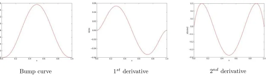
If the class parameters N1 and N2 are set to 3, and the shape function S(ψ) = 1, as in equation (22), a bump like curve is obtained with 1st and 2nd derivatives of zero at starting and ending points. The curve
and 1stand 2ndderivative distribution are shown in Figure 1.
ξ(ψ) =ψ3.0·(−1)ψ3.0 (22)
The above figures clearly show that the geometry, 1st and 2nd derivatives are all zero at the start and end
position of the bump. In addition, because the class parameters are exponential parameters of the class
function, if N1 and N2 are set to 3, the bump peak value reduces to 1/64 for the shape functionS(ψ) = 1. Because the bump maximum height and bump peak crest position parameters do not directly appear in
the CST function, the shape function parameter values should be a similar magnitude to bump height.
Multiplying by 64 in the CST equation moves the peak value back to 1 when S = 1. This is convenient
Bump curve 1stderivative 2ndderivative
Figure 1: Bump curve and derivatives using the CST parameterisation method
for the user when setting up their design parameter range. The full description of the 2D CST bump with
shape function is:
ξ(ψ) =64·C33.0
.0(ψ)·
n
X
i
Ai·Si(ψ)
CN1
N2(ψ) =ψ
N1·(1−ψ)N2
Si(ψ) = n
X
r=0
Kr,nψr(1−ψ)n−r
Kr,n=
n r
= n!
i!(n−i)!
x=ψ·xlength
z=ξ·xlength
The three-dimensional bump is the extension of two-dimensional bump using a second Bernstein polynomial.
Finally, the bump patch may not be strictly a rectangle, so the bump length distribution along spanwise is
a function of span. The definition of a three-dimensional bump with sweep angle is shown in the following
equations:
ξ(ψ, η) = 64·C33.0
.0 ·
Nx
X
i Ny
X
j
[Bi,j·Sxi(ψ)·Syj(η)]·H(η)
where
H(η) =64·C3.0 3.0(η)·
n
X
i
Ai·Si(η)
x=xleading(y) +ψ·xlength(y)
y=η·ywidth
z=ξ
xlength(y) =(xleading(y)−xtrailing(y)
where xleading and xtrailing are the leading edge and trailing edge values of x at a giveny, which can be
a higher polynomial function depending on the distribution shape. The CST bump equations can provide
higher flexibility of a local bump, and generate symmetric or asymmetric bumps in three-dimensional space.
The orders of Bernstien polynomials are recommended to be below 4, this allows the CST bump to provide
high flexibility with a reasonable number of design variables and produce the most realistic bump shapes. As
stated in the previous section, the flow solver and adjoint solver used is TAU developed by DLR. TAU is a
hexahedral dominant multi-grid solver.15 The meshes of all the geometries use hexahedral dominant hybrid
meshes which are generated using Solar which has been developed by the Aircraft Research Association, BAE
System and Airbus.16 Once the gradient is obtained, a SLSQP21, 22 optimizer from the NLOPT package23
is employed to perform optimization.24 One test case, the M6 wing, is analysed throughout. This case has
been widely used in the area of aerodynamic research.25, 26
IV.
Three-dimensional Bump deployment and Optimization
IV.A. M6 Surface Sensitivity
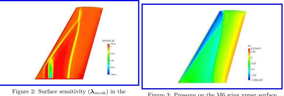
In this case, the flow condition is chosen as Mach=0.84, Re=11.72×10⁶ and Cl=0.2743. The mesh adjoint is first to be calculated for a zero height bump, i.e. there is no deformation of the mesh. In bump design,
the surface points in the bump area are only moving along the z-direction. Therefore, only λmesh,z (also
referred to as lambda gz) is used. λmesh,z are the sensitivities ofCd respect to changes of the surface in the
z-direction. The contour ofλmesh,z is plotted in Figure 2.
Figure 2 shows the negative surface sensitivity on the upper surface of the M6 wing. The green,blue and
yellow areas on the surface in figure 2 show regions where the derivative points in a positive z-direction.
The red regions show areas with negative or very small gradients. On the M6 wing the sensitivity makes
a clear lambda structure. The pressure plot confirms that the lambda structure can be attributed to the
Figure 2: Surface sensitivity (λmesh) in the
z-direction Figure 3: Pressure on the M6 wing upper surface
shock locations. In addition to this there is a non-shock region near the wing root which suggests moving
the surface in a positive z-direction in that region could also achieve a drag change.
Previous research27has focussed on optimising a shock bump array on the rear shock line only (neglecting
near the tip); this paper takes this further by applying the bumps over the entire span of the wing.
Further-more, it explores surface changes in the front shock region and the sensitive non-shock region near the wing
root.
IV.B. Rear Shock Line
The surface mesh points with large negativeλmesh value, shown in blue, green and yellow colour in Figure
2. The rear shock line shows the greatest potential for shock bump deployment as it shows the greatest
sensitivities of the two shock lines. The rear shock line is extracted then the points are fitted and smoothed
using 5thorder polynomials. The sensitivities feature line is then obtained.
In this subsection only the rear shock line is considered, however, in later sections other areas will be analysed.
It is particularly important to involve the wing tip region where the sensitivity is strongest. The bump is
deployed starting at y=0.01m and ending at y=1.19m. 14 bumps are evenly distributed, which gives a bump width of 0.084m. The optimisation region is defined by a front line and rear line. The distance between these lines is defined byxlength(y) = 0.35×Chordwing(y). This means at any span position, the local length of the
bump is equal to 35% wing local chord. This is based on previous research by Wong7 and Qin et al,8which
suggested that the shock control bump length should be between 20% to 40% chord length. Finally, the
bump has to be deployed with respect to the shock feature line. The EUROSHOCK II project6 suggested
that the peak of shock control bump should be between 5−10% downstream of the shock for an asymmetric
bump. The bump will be placed downstream in terms of shock feature line. In this case, it has 40% length
in front of shock feature line and 60% behind. Figure 4 shows the bounds of the optimisation region.
[image:12.612.72.545.51.211.2]Figure 4: Extraction of rear shock sensitivity data with curve fitting and subsequent front and rear optimisation bounds
After the bump area is decided, the optimization can be carried out. In this case, the Bernstein polynomials
for each bump has 3rd order on chordwise, 3rd order on spanwise, and 3rd order to control shape function
of the height distribution. The length and width of the bumps are fixed, hence the total number of design
variables is 14×((4×4) + 4) = 280.
During the flow calculation the lift is fixed to guaranteeCl is matched with the requirement, the objective
function is then modified as:
minI=Cd− ∂Cd
∂α
∂Cl
∂α
(Cl−Cl,target) (23)
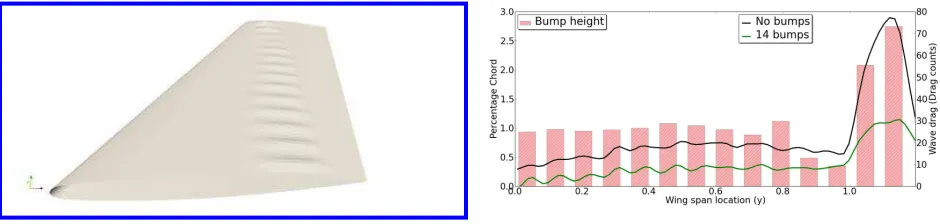
Figure 5 shows the topology of the bumps on the M6 wing of the final iteration in the optimisation. It is
obvious that at the tip the bumps are the tallest, this is what we would expect since the sensitivities in the
positive z-direction at this location are very strong. It is also interesting to note that at the region where
the ‘legs’ of theλ-shock concatenate the shock bump height is very close to zero. In this region the possible reduction of wave drag for one of the shocks is offset by an increase of drag elsewhere, therefore the optimiser
has driven the bump height to be smaller in this region. The highest bumps are found at the tip region on
the wing where the wave drag is largest. The wave drag has been reduced all across the span when bumps
are present, however at the tip there is still a significant amount of wave drag generated which could further
be reduced.
Figures 6 and 7 show the surface pressure distribution on the upper surface of the M6 wing. The M6 wing
with no bumps shows a very sharp change in pressure at the rear shock line which is not present in the
case with the optimised bumps included. When the optimised bumps are placed on the wing the pressure
M6 wing with optimised bumps Percentage height distribution and spanwise wave drag
Figure 5: Bump distribution and spanwise wave drag
change in the rear shock line region is much more gradual across the majority of the span. At the wing tip
the pressure change has been reduced in most of the tip area but there is still a small area in between the
bumps which contains a sharp change in pressure which is indicative of a small shock.
[image:14.612.71.545.289.436.2]Figure 6: M6 wing upper surface pressue distribution with no bumps
Figure 7: M6 wing pressure distribution with 14 bumps
Figure 8 shows spanwise slices along the M6 wing and the surace pressure distribution is plotted on each
slice. For the 1st through to the 11th bump the pressure distribution at the rear shock shows a much more
gradual change, this effect on the pressure distribution is typical of a well designed shock bump. The 12th
bump is in the region when the front and rear shocks join, there is still a positive effect on the rear shock
but it is much less significant in comparison to the bumps closer to the wing root. For bumps 13 and 14
at the wing tip there is a strong re-expansion of the flow after the initial compression, however the pressure
change after the re-expansion is not as severe. Between the 13thand 14ththere is a strong re-expansion of
the flow and the gradient of pressure after the re-expansion is still large, indicative of a shock.
Table 1 shows a comparison of the drag decomposition using the far field drag analysis tool FFD72.28 When
the bumps are deployed the drag is reduced by just less than 19 drag counts. The table also shows that
the pressure drag reduces while the skin friction shows a slight increase which is common when using shock
bumps.
1st bump 2nd bump
7th bump Between 7th and 8thbump
11th 12thbump
13thbump Between 13th and 14thbump
[image:15.612.71.543.50.693.2]14thbump
Figure 8: Streamwise surface slices showing the pressure distribution on the surface
Table 1: Far field drag comparison between optimised shock bump and no bump cases
(drag counts) Cd,total Cd,wave Cd,induced Cd,viscpres Cd,f riction CCdl
NoBump 175.87 28.69 62.24 31.13 52.69 15.55 14 bumps 156.91 12.81 62.31 27.80 53.56 17.42 Reduction -10.78% -55.35% 0.11% -10.70% 1.65% 12.03%
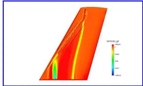
Figures 9 and 10 show the surface sensitivity for the upper surface of the M6 wing with no bumps and
after the optimisation is applied. For most of the span the sensitivity of drag to changes in the surface has
been reduced significantly in the rear shock area. The only area to still show a strong sensitivity in the
optimisation region is between the two bumps at the tip of the wing. A possible explanation for this is that
the shock is so strong in this location that the bumps cannot grow high enough to treat it without incurring
a drag penalty elsewhere. This shows that there is a need to improve the parameterisation method such that
a shape can be found that will act directly on this region. It is intersting to note that in this comparison
the non-shock sensitivity region is reduced after the bump optimisation despite no optimisation taking place
in the local vacinity. This indicates that the surface in the rear shock and non-shock region are somehow
[image:16.612.75.543.343.514.2]linked.
Figure 9: Surface sensitivity of M6 wing with no bumps
Figure 10: Surface sensitivity for final iteration of optimisation
IV.C. Leading Shock Line
The previous subsection focusses on the application of shock bumps in the rear shock region across the entire
wing span, this subsection will focus on the other shock line near the leading edge (LE). The future of this
research will look into combining all of these regions together into a unified optimisation, therefore the tip
region after the shock legs join is not considered as part of the LE optimisation region. A further limitation
to this case is that the mesh deformation scheme fails when adding bumps too close to the wing leading
edge. This is due to the fact that the clustering of nodes at the wing leading edge is dense and the change
from adding bumps can create poor quality cells at the leading edge.
Figure 11 shows the optimisation region considered for this case. Due to the proximity of the leading edge
a much shorter bump is used compared to that of the previous section, the optimisation region is 25% local
chord in streamwise length, this is still within the suggested length. There will be 8 bumps deployed with a
[image:17.612.157.448.150.324.2]bump width of 0.056m each. The optimisation region begins aty= 0.5m and ends aty= 0.95m. As with the previous test case each bump will have 40% before the feature line and 60% after.
[image:17.612.75.539.422.531.2]Figure 11: Extraction of leading edge shock sensitivity data with curve fitting and subsequent front and rear optimisation bounds
Figure 12 shows the final optimised bump array on the leading shock edge. Although bumps have established
themselves in this region the height of the bump is small and therefore the effect on the wave drag is minimal.
M6 wing with optimised bumps Percentage height distribution from root (left) to tip (right)
Figure 12: Bump distribution and spanwise wave drag distribution
Figures 13 and 14 show the pressure distributions with no bump and with optimised bumps. The bumps
here have had a small effect on weakening the pressure peak in the shock location but there still remains a
significant pressure change in the front shock line region.
Figure 15 shows spanwise slices of the wing with the surface pressure distribution plotted at each slice.
Between the 1st and 4th bumps there is little effect on the front shock. Bumps 5 through 8 shows a much
more gradual pressure change in the shock region. For the entire shock array there is no effect downstream
Figure 13: M6 wing upper surface pressue distribution with no bumps
Figure 14: M6 wing pressure distribution with bumps placed on leading shock line
at the rear shock. The bottom two pressure distributions show that there is only a local effect of LE bump
array.
Table 2 shows the comparison of drag values for total, pressure and skin friction drag. This shows that the
application of the shock bumps in this region has only had a small change on the drag. The bumps were
placed in a region where the sensitivity was not as strong and due to the limitations on the placement, this
[image:18.612.123.491.395.453.2]could explain why the drag has not reduced by a substantial amount.
Table 2: Far field drag comparison between optimised shock bump and no bump cases
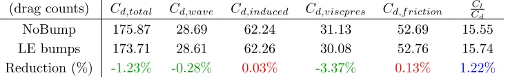
(drag counts) Cd,total Cd,wave Cd,induced Cd,viscpres Cd,f riction CCdl
NoBump 175.87 28.69 62.24 31.13 52.69 15.55 LE bumps 173.71 28.61 62.26 30.08 52.76 15.74 Reduction (%) -1.23% -0.28% 0.03% -3.37% 0.13% 1.22%
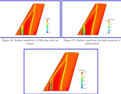
Figures 16 and 17 show the surface sensitivity in the z-direction with no bumps and with the optimised
bumps. The optimised bumps have had an effect on the sensitivity in the optimisation region, however the
stronger sensitivity regions are closer to the wing root.
IV.D. Non-Shock region
This paper so far has focussed on optimisations in the shock regions, the subsection will look into an area
where there is not a shock but the sensitivity map suggests that a change in the surface in the positive
z-direction will have a strong effect on the drag.
Figure 18 shows the optimisation region considered for this case. The optimisation region is 25% local chord
in streamwise length. There will be 4 bumps deployed with a bump width of 0.085meach. The optimisation region begins aty= 0.01mand ends aty= 0.35m. As with the previous test case each bump will have 40% before the feature line and 60% after.
1st bump Between 1st and 2nd bump
3rd bump Between 3rd and 4th bump
5th bump 6th bump
7th bump 8th bump
[image:19.612.69.548.51.710.2]1 bump width toward the wing root 2 bump widths toward the wing tip Figure 15: Streamwise surface slices showing the pressure distribution on the surface
Figure 16: Surface sensitivity of M6 wing with no bumps
Figure 17: Surface sensitivity for final iteration of optimisation
Figure 18: Extraction of non-shock sensitivity data (at the wing root) with curve fitting and subsequent front and rear optimisation bounds
Figure 19 shows the topology of the optimised bumps. All 4 bumps have grown to a similar height at
approximately 0.5% local chord. When the bumps are present the wave drag is reduced from the root to
y = 0.9m. At y = 0.9mthe the wave drag dramatically increases due to the concatenation of the leading edge and rear shock lines. This concatenation point is further from the tip than in the no bump case and
causes the wave drag at the tip to be slightly stronger.
Figures 20 and 21 show the surface pressure distribution on the upper surface of the M6 wing. The
in-troduction of the optimised bumps has introduced an increase in pressure in the local region and directly
downstream of the bumps the pressure change is much less dramatic. In addition to this the bump furthest
down the span is acting slightly on the front shock line.
The surface pressure at various slices along the wing span in figure 22 show that there is a compression
then expansion caused by the placement of bumps 1, 2 and 3. The placement of bump 4 has forced extra
compression of the flow around the front shock line. The placement of these bumps has moved the rear
M6 wing with optimised bumps Percentage height distribution and spanwise wave drag
Figure 19: Bump distribution and spanwise wave drag
[image:21.612.70.543.222.365.2]Figure 20: M6 wing upper surface pressue distribution with no bumps
Figure 21: M6 wing pressure distribution with bumps placed in the non-shock sensitvity region
shock line slightly upstream of its original location causing the two shock lines to join earlier and directly
downstream of the optimisation region the shock is weaker.
Table 3 shows the comparison of total, pressure and skin friction drag between the optimised and no bump
case. The drag reduction after the bumps are deployed is 4 drag counts and interestingly the skin friction
[image:21.612.115.495.541.601.2]barely changes.
Table 3: Far field drag comparison between optimised shock bump and no bump cases
(drag counts) Cd,total Cd,wave Cd,induced Cd,viscpres Cd,f riction CCdl
NoBump 175.87 28.69 62.24 31.13 52.69 15.55 Non-shock bumps 170.68 26.01 62.21 29.80 52.66 16.02 Reduction -2.95% -9.34% -0.05% -4.27% -0.057% 3.02%
Figures 23 and 24 show the surface sensitivity in the z-direction for the M6 wing with no bumps and the
M6 wing with optimised bumps. After the bumps are deployed the sensitivity downstream of the bumps at
the rear shock line has been reduced. The sensitivity in the non-shock region has been reduced significantly
but the sensitivity map does suggest that increasing the bump length may give even more drag reduction.
Since the front shock line and the non-shock region are so close a combined array may prouduce a better
1st bump Between 1st and 2nd bump
2nd bump Between 2ndand 3rd bump
3rd bump Between 3rd and 4th bump
4th bump Half bump width after 4thbump
[image:22.612.70.544.51.709.2]2 bump widths downstream 4 bump widths downstream Figure 22: Streamwise surface slices showing the pressure distribution on the surface
drag reduction over all.
[image:23.612.71.543.69.236.2]Figure 23: Surface sensitivity of M6 wing with no bumps
Figure 24: Surface sensitivity for final iteration of optimisation
IV.E. Entire sensitivity region optimisation
This paper has looked at individual regions for optimisation of bumps. In this section bumps will be placed
and optimised in all the sensitivity regions.
Figure 25 shows the optimisation region considered for this case. The optimisation region for the leading
edge is 25% local chord in streamwise length and 35% for the rear region. There will be 26 bumps deployed,
9 bmps each in the front and rear regions and 7 in the concatenated region near the wing tip. The bumps
in the leading and rear regions have bump width 0.0826mand the bumps in the concatenated region have bump width 0.0624m. The optimisation region begins aty = 0.01m and ends at y = 1.19m. As with the previous test case each bump will have 40% before the feature line and 60% after. The concatenated region
[image:23.612.154.448.491.666.2]begins at 0.753m from the root of the wing.
Figure 25: Extraction of sensitivity data with curve fitting and subsequent front and rear optimisation bounds
Figure 26 show the topology of the optimised bumps and the bump heights for each optimisation region and
the comparison of wave drag between the current case, the no bump case and the rear-shock line case. For
the LE region and rear optimisation region the bump patches in line in the spanwise direction, therefore the
bump heights are offset from each other in the bar chart for clarity. For the current case the wave drag is
reduced a little more in the mid span of the wing compared to the rear-shock line case however this will be
somewhat offset by the increase in wave drag toward the tip region.
[image:24.612.71.540.180.287.2]M6 wing with optimised bumps Percentage height distribution and spanwise wave drag
Figure 26: Bump distribution and spanwise wave drag
Figures 27 and 28 show the surface pressure distribution on the upper surface of the M6 wing. The
introduc-tion of the optimised bumps shows a much more gradual pressure change in the rear shock region, however
the bumps in the non-shock region have not had as large an effect as in section IV.D. This may be due to
the weakening of the sensitivity in this region shown in the final iteration of the rear shock line optimisation
[image:24.612.74.543.439.591.2]in section IV.B.
Figure 27: M6 wing upper surface pressue distribution with no bumps
Figure 28: M6 wing pressure distribution with bumps placed in all the sensitvity regions
Figure 29 shows spanwise slices along the wing where the surface pressure has been plotted. For the 1st and
2ndbumps the effect from the non-shock region bump causes a small compression and expansion in the fluid.
The bumps further downstream act on the rear shock by making the pressure change much more gradual.
By the 4thbump, the effect of the bump in the non-shock region is negligible, this is due to the small height
of the bump. From the 6th to the 11thbump the pressure distribution at the front and rear shock is either
much more gradual or the pressure peak before the shock is significantly reduced. For bumps 14 through
16 the pressure distribution exhibits a small re-expansion of the flow, however the pressure peak does not
return to the strength of the baseline case.
Table 3 shows the comparison of total, pressure and skin friction drag between the optimised and no bump
case. Comparing tables 4 and 2, the overall drag reduction is 1 drag count better than when using optimised
[image:25.612.91.518.221.334.2]bumps in the rear-shock region alone.
Table 4: Far field drag comparison between optimised shock bump and no bump cases
(drag counts) Cd,total Cd,wave Cd,induced Cd,viscpres Cd,f riction CCdl
NoBump 175.87 28.69 62.24 31.13 52.69 15.55
14 bumps 156.91 12.81 62.31 27.80 53.56 17.42
Reduction from NoBump -10.78% -55.35% 0.11% -10.70% 1.65% 12.03%
All region bumps 155.33 12.39 62.33 26.93 53.68 17.60 Reduction from NoBump -11.68% -56.81% 0.15% -13.49% 1.88% 13.18%
Figures 30 and 31 show the surface sensitivity in the z-direction for the M6 wing with no bumps and the
M6 wing with optimised bumps. After the bumps are deployed the sensitivity downstream of the bumps at
the rear shock line has been reduced. The sensitivity in the non-shock region has been reduced significantly
but the sensitivity map does suggest that increasing the bump length may give even more drag reduction.
Since the front shock line and the non-shock region are so close a combined array may prouduce a better
drag reduction over all.
V.
Conclusion
The mesh adjoint method has been used throughout this paper as a design tool to aid in the placement
and optimisation of flow control device. For purely geometric optimisations a by-product of obtaining the
gradients of the objective function with respect to the design variables is finding the sensitivity of the
objective function with respect to surface changes. This value is the solution to the mesh adjoint equation
−λmesh.
This work has focused on the M6 wing test case. The sensitivity produced from this case is very diverse and
therefore shows how the mesh adjoint can aid a designer. The flow over the M6 produces a shock with a
front and rear shock leg, both of which have been analysed and shock bumps have been optimised to treat
the production of wave drag in these regions.
1st bump 2nd bump
4th bump 6th bump
9th bump Between 9thand 10thbump
11thbump 14thbump
[image:26.612.74.540.52.716.2]Between 14th and 15thbump 16thbump
Figure 29: Streamwise surface slices showing the pressure distribution on the surface
Figure 30: Surface sensitivity of M6 wing with no bumps
Figure 31: Surface sensitivity for final iteration of optimisation
An interesting region of sensitivity was also discovered on the upper surface of the M6 wing. This region
was shock free but the sensitivity map indicated that a surface change in the positive z-direction would give
a change in the drag. Using the existing framework, bumps where added into the non-shock region. It was
found that the optimised bumps reduced the change in entropy at the shock directly downstream from the
optimisation region.
The final analysis considered placing bumps in all the sensitivity regions on the M6 wing upper surface and
optimising. In a comparison with the rear-shock region case, using all the sensitivity regions gained an extra
reduction in drag by 1 drag count.
A higher drag reduction could be found if the parameterisation was improved in the non-shock region and
the tip region such that all the sensitivity in those regions is reduced.
VI.
Acknowledgements
The author would like to thank Feng Zhu for creating the optimisation framework and the helpful discussions
thoughout this papers research.
The work was supported by the ESPRC/Airbus ICASE award. The author would like to thank Airbus for
their help throughout this investigation.
VII.
References
References
1
Fulker, J. L., Ashill, P. R., and Simmons, M. J., “Study of simulated active control of shock waves on an aerofoil,”Technical
Report 93025 DERA, May 1993.
2
Ashill, P. R., Fulker, J. L., and Shires, A., “A novel technique for controlling shock strength of laminar flow aerofoil sections,”
First European Symposium on Laminar Flow, Hamburg, March 1992.
3
Fulker, J. L., Ashilll, P. R., and Simmons, M. J., “Computational Study of Shock Control at Transonic Speed,”PhD Thesis,
Cranfield University, 2000.
4
Lutz, T., Kutzbach, M., and Wagner, S., “Investigations on shock control bumps for infinite swept wings,”AIAA 2004-2702,
2004.
5
Birkemeyer, J., Rosemann, H., and Stanewky, E., “Shock control on swept wing,”J. Aerospace Sci and Tech, 2000, pp. 147–
156.
6
Stanewsky, E., Delery, J., Fulker, J. L., and De Matteis, P., “Drag reduction by shock and boundary layer control, Results
of the project EUROSHOCK II, Notes on Numerical Fluid Mechanics and Multidisciplinary Design,”Springer, 1997.
7
Wong, W. S., Le Moigne, A., and Qin, N., “Parallel adjoint-based optimisation of a blended wing body aircrft with shock
control bumps,”Aeronautical Journal, Vol. 111, 2007, pp. 165–174.
8
Qin, N., S., W. W., and Le Moigne, A., “Three-dimensional contour bumps for transonic wing drag reduction,”J. Aerospace
Engineering, Vol. 222, 2008, pp. 619–629.
9
S., W. W., “Mechanisms and Optimisations of 3D Shock Control Bumps,”PhD Thesis, The University of Sheffield, 2006.
10
Lions, J. L., “Optimal Control of Systems Governed by Partial Differential Equations,”Springer-Verlag, New York, Translated
by S.K. Mitter, 1971.
11
Pironneau, O., “On optimum profiles in Stokes flow,”Journal of Fluid Mechanics, Vol. 59, 1973, pp. 117–128.
12
Jameson, A., “Aerodynamic design via control theory,”National Aeronautics and Space Administration, Langley Research
Center, 1988.
13
Nielsen, E. J. and Park, M., “An Adjoint Approach to Eliminate Mesh Sensitivities in Computational Design,”AIAA
2005-491, 2005.
14
Kulfan, B. M. and Bussoletti, J. E., ““Fundamental” Parametric Geometry Representations for Aircraft Component Shapes,”
AIAA 2006-6948, 2006.
15
Gerhold, T., Friedrich, O., and Evans, J., “Calculation of complex three-dimensional configurations employing the DLR-TAU
code,”AIAA 1997-167, 1997.
16
Leatham, M., Stokes, S., and Shaw, J. A., “Automatic mesh generation for rapid-response Navier-Stokes calculations,”AIAA
2000-2247, 2000.
17
Le Moigne, A., “A discrete Navier-Stoked adjoint method for aerodynamic optimisation of Blended Wing-Body
configura-tions,”PhD Thesis, The University of Sheffield, 2002.
18
Dwight, R., “Robust Mesh Deformation using the Linear Elasticity Equations,”Computational Fluid Dynamics, Springer
Berlin Heidelberg, 2009, pp. 401–406.
19
Ilic, C., Widhalm, M., and Brezillon, J., “Efficient Polar Optimization of Transport Aircraft in Transonic RANS Flow Using
Adjoint Gradient Based Approach,” European Congress on Computational Methods in Applied Sciences and Engineering
(ECCOMAS), 2012.
20
Widhelm, M., Brezillon, J., Ilic, C., and Leicht, T., “Investigation on Adjoint Based Gradient Computations for Realistic 3d
Aero-Optimization,”AIAA 2012-9129, 2010.
21
Krafter, D., “A software package for sequential quadratic programming,”Technical Report DFVLR-FB 88-28, Institut fr
Dynamik der Flugsysteme, Oberpfaffenhofen, July 1988.
22
Krafter, D., “Algorithm 733: TOMPFortran modules for optimal control calculations,”ACM Transactions on Mathematical
Software, Vol. 20, No. 3, 1994, pp. 262–281.
23
Johnson, S. G., “The NLopt nonlinear-optimization package,” http://ab-initio.mit.edu/nlopt.
24
Nocedal, J. and Wright, S. J., “Numerical Optimization,”London: Springer, Vol. 2nd ed, 2006.
25
Schmitt, V. and Charpin, F., “Pressure Distributions on the ONERA M6 Wing at Transonic Mach Numbers,”Experimental
Database for Computer Program Assessment AR-138, B1-1-B1-44, AGARD, May 1979.
26
Durrani, N. and Qin, N., “Comparison of RANS, DES and DDES results for ONERA M6 Wing at transonic flow speed using
an in-house parallel code,”AIAA 2011-190, 2011.
27
Zhu, F., Hinchliffe, B., and Qin, N., “Using Mesh Adjoint for Shock Bump Deployment and Optimization on Transonic
Wings,”AIAA SciTech, 2015.
28
Destarac, D., “Far-eld/near eld drag balance and applications of drag extraction in cfd,”VKI Lecture Series, 2003, pp. 3–7.
29
Nielsen, E. J., Diskin, B., and Yamaleev, N., “Discrete Adjoint-Based Design Optimization of Unsteady Turbulent Flows on
Dynamic Unstructued Grids,”AIAA 2009-3802, 2009.
30
Brezillon, J. and Dwight, R. P., “Discrete Adoint of the Navier-Stokes Equations for Aerodynamic Shape Optimization.
Evolutionary and Deterministic Methods for Design,”EUROGEN Conference, 2005.
31
Brezillon, J., Ronzheimer, A., Haar, D., Abu-Zurayk, M., and Lummer, M., “Development and application of
multi-disciplinary optimization capabilities based on high-fidelity methods,”AIAA 2012-1757, 2012.