c
Communications in Mathematical Sciences (2014)A Convex and Selective Variational Model for Image
Segmentation
Jack Spencer∗and Ke Chen∗†
Abstract
Selective image segmentation is the task of extracting one object of interest from an image, based on minimal user input. Recent level set based variational models have shown to be eective and reliable, although they can be sensitive to initialization due to the mini-mization problems being nonconvex. This sometimes means that successful segmentation relies too heavily on user input or a solution found is only a local minimizer, i.e. not the correct solution. The same principle applies to variational models that extract all objects in an image (global segmentation); however, in recent years, some have been successfully reformulated as convex optimization problems, allowing global minimizers to be found.
There are, however, problems associated with extending the convex formulation to the current selective models, which provides the motivation for the proposal of a new selective model. In this paper we propose a new selective segmentation model, combining ideas from global segmentation, that can be reformulated in a convex way such that a global minimizer can be found independently of initialization. Numerical results are given that demonstrate its reliability in terms of removing the sensitivity to initialization present in previous models, and its robustness to user input.
Keywords. Image processing, Variational segmentation, Level set function, Edge detection, Convex functional, Euler-Lagrange equation, AOS.
AMS subject classications. 62H35, 65N22, 68U10, 35A15, 65C20, 74G65, 74G75.
1 Introduction
An important part of Image Processing is segmentation; the task of partitioning an image into multiple regions (each sharing certain characteristics - such as texture, intensity, shape, colour etc.). Given an imagez(x, y) in a bounded domain Ω⊂R2, we look for an edge Γ that
partitionsΩinto regions{Ωi, i= 1,2, ..., l}inΩ\Γ. Within Segmentation, there is the global
approach and the local approach. Global segmentation is the task of selecting all objects in an image based on a certain characteristic, e.g. intensity, and has been widely studied over the last twenty years [9, 21]. Selective segmentation is when only one object, from within all objects, is selected [1, 27].
∗Centre for Mathematical Imaging Techniques and Department of Mathematical Sciences, University of
Liverpool, United Kingdom. Email: [email protected], Web: www.liv.ac.uk/cmit
We consider the variational approach to these problems. Within variational segmentation techniques two main ideas have developed: edge-based methods and region-based methods. An important region-based method, where the idea is to achieve segmentation through an approximation of the original image, is the Mumford-Shah functional minimization [22]; there exists a large literature extending this work. Edge-based methods drive an evolving contour towards edges within an image using an edge detector function. This method was originally proposed by Kass et al. [17]; further work by Caselles et al. led to the Geodesic Active Contours model [5]. Recently, in order to incorporate the advantages of each idea, there has been a tendency to combine edge-based and region-based approaches [19, 5].
The requirements for a selective segmentation model are that solutions are computed quickly and they are reliable with minimal user input. Much research has been done in recent years on developing this idea. In 2005, Gout, Le Guyader and Vese [14] introduced geometrical constraints to Geodesic Active Contours similar to [5] in the form of a set of points on the contour of interest. This idea was enhanced further by Badshah and Chen [1] in 2009, by combining this work with the region-based idea of Mumford-Shah [22] and Chan-Vese [10]. In 2011, to increase model reliability, Rada et al. [27] introduced a novel Dual Level Set Model, where a local level set incorporates geometrical constraints similar to [14] and [1], locating an object within a global level set. The selective model discussed in detail here is the Rada-Chen model [28], introduced in 2012 to improve on [27] by using a single level set function, where there is a constraint introduced on the area inside the contour. This has proven to be the most eective model. Another idea of improving [1], that is not of the same type as [22], was proposed by Badshah and Chen [2] in 2012, incorporating tting based on coecient of variation.
These models, either global or selective, are nonconvex, which can lead to problems in the form of local minima. This means that nding the correct solution is dependent on initializa-tion, which reduces their reliability. In recent years work has been done to reformulate global segmentation models as convex minimization problems such that any local minimizer is a global minimizer. The focus of this paper is to apply the convex reformulation of nonconvex global models to selective segmentation. We remark that one of the current challenges in global seg-mentation is reformulation into convex or relaxed models for multiphase cases [18, 15, 6, 3]. Other challenges include the idea of selective segmentation based on user input of 3-D images. Chan-Vese has been generalized to 3-D by Zhang and Chen [31], and user input of a similar type to [1, 28, 14] has been applied with active contours in 3-D by Le Guyader and Gout [13]. This involves the selection of points on slices of the 3-D data. Visualising objects in this way, allowing for ecient user input, is a dicult problem. In relation to Rada-Chen [28], this input would generate a polyhedron, with its volume providing a selection constraint.
both the nonconvex and convex models. Conclusions of the paper are given in Section 6.
2 Global Segmentation
In order to discuss the selective segmentation methods of interest, it is important to introduce global variational image segmentation models. This is important for two reasons; rstly, it will provide the foundation for the selective models introduced and secondly, it provides the method for minimizing the associated functionals with the introduction of Active Contours Without Edges [10] by Chan and Vese in 2001.
2.1 The Mumford-Shah Approach
One of the most important variational image segmentation models is by Mumford and Shah [22], introduced in 1989, and forms the basis for this work as well as many others. Let Ω be
a bounded domain in Rn and z be a bounded measurable function dened on Ω. Here we
consider the case where n= 2. In the piecewise constant case, the image, z, is reconstructed
as a cartoon of the original where each region, Ωi, consists of homogeneous intensity (with
i= 1, . . . , l), separated by an edge setΓ, a closed subset ofΩ.
In 2001, Chan and Vese [10] introduced a particular case of the piecewise constant Mumford-Shah functional. This was the two-phase example (l = 2), with Ω1 =in(Γ) and Ω2 =out(Γ), which looks for the best approximation of an image zby a function u taking only 2 values,
u=
c1=average of z insideΓ,
c2=average of z outsideΓ.
The length of the setΓ is given by
|Γ|= Z
Γ
ds.
The piecewise constant two-phase Mumford-Shah (P C) functional is given as follows:
P C(Γ, c1, c2) =µ|Γ|+λ Z
in(Γ)
(z−c1)2dΩ +λ Z
out(Γ)
(z−c2)2dΩ. (2.1)
It consists of the regularization term, |Γ|, forcing the boundary between homogeneous regions to be as short and as smooth as possible, and the tting terms which force the boundary to nd regions of homogeneous intensity. Theoretical existence and regularity of minimizers of the P C case (2.1), with respect to Γ, are discussed in [22]. However, minimizing P C (2.1)
is problematic due to the diculty of tracking the movement of Γ and the model was not
implemented directly until the work of [10].
2.2 The Chan-Vese Method
and Vese proposed to replace the unknown 1-D variable with a higher dimensional variable, counterintuitively simplifying the problem. They applied the level set method [26], introduced by Osher and Sethian in 1988, to (2.1). By tracking a variable of a higher dimension, where the boundary is represented by a level set of this variable, topological changes in the boundary, such as splitting into two or merging into one, are dealt with automatically. Formally, the boundaryΓ is represented by the zero level set of the Lipschitz functionφsuch that
Γ ={(x, y)∈Ω φ(x, y) = 0},
in(Γ) ={(x, y)∈Ω φ(x, y)>0},
out(Γ) ={(x, y)∈Ω φ(x, y)<0}.
TheP C functional (2.1) is reformulated using the Heaviside function H and the Dirac deltaδ
dened by
H(φ(x, y)) =
1, if φ(x, y)≥0
0, if φ(x, y)<0, δ(φ(x, y)) =H
0(φ(x, y)).
In order to compute the associated Euler-Lagrange (EL) equation forφwe consider regularized
versions ofH andδ, given as
H(φ) =
1 2
1 + 2
π arctan φ
, δ(φ) =
1
π(1 +φ2/2). TheP C functional (2.1) is then reformulated as follows:
CV(φ, c1, c2) =µ Z
Ω
δ(φ)|∇H(φ)|dΩ +λ
Z
Ω
(z−c1)2H(φ)dΩ
+λ
Z
Ω
(z−c2)2(1−H(φ))dΩ, (2.2)
whereφ(x, y)has been replaced withφfor simplicity; this notation will be continued from here.
Minimizing (2.2) with respect to the intensity constants c1 and c2 is given by:
c1(φ) = R
ΩH(φ)z dΩ R
ΩH(φ)dΩ
, c2(φ) = R
Ω(1−H(φ))z dΩ R
Ω(1−H(φ))dΩ
. (2.3)
Then, given these constants, (2.2) is minimized with respect toφ:
min
φ CV(φ, c1, c2) (2.4)
This leads to the EL equation
(
µδ(φ)∇ ·
∇φ
|∇φ|
−λδ(φ)
(z−c1)2−(z−c2)2
= 0 inΩ,
∂φ
∂~n = 0 on∂Ω.
characteristic functions. This means that there are local minima and a computed solution may not be correct unless the initial guess is suciently close to the true solution. Fortunately, by reformulating as the minimization of a convex functional, global minimizers of the nonconvex problem (2.4) can be found. This idea has not yet been applied to selective segmentation models, which also have local minima.
2.3 A Global Convex Reformulation
Important to the idea of reformulating a model to be convex is why this improves the reliability of a solution. With that in mind, the fundamental idea behind convex minimization is now discussed briey in a general sense. Consider the problem of minimizingf(x)subject tox∈S,
given a non-empty setS. A point x∈S is called a feasible solution to the problem. If ¯x∈S
and f(x) ≥ f(¯x) for each x ∈ S, then ¯x is a global minimum. If ¯x ∈ S and there exists an -neighbourhoodN(¯x)around¯xsuch thatf(x)≥f(¯x)for eachx∈S∩N(¯x), thenx¯is called
a local minimum.
The advantage of convex minimization is that supposingx¯is a local minimum, iff is convex
and S is a convex set, then ¯x is a global minimum. It has been shown that minimizing the
piecewise constant two-phase Mumford-Shah functional with respect toΓ can be reformulated
as a convex problem, by relaxation of the label set. We now introduce the theory behind reformulating the functional (2.1), which we shall later apply to selective segmentation.
We consider the minimization of the piecewise constant two-phase Mumford-Shah functional from (2.1) with respect toΓ; reformulated to the minimization problem (2.4) by Chan and Vese
[10]. Observe that
CV(φ, c1, c2) =µ Z
Ω
δ(φ)|∇H(φ)|dΩ +λ
Z
Ω
(z−c1)2H(φ)dΩ +λ Z
Ω
(z−c2)2(1−H(φ))dΩ
is nonconvex due to the presence of H(φ). In 2006, Chan, Esedoglu and Nikilova [8] proposed
replacing H(φ) with u ∈ [0,1] in (2.2), and obtained the following equivalent, convex, and
constrained minimization problem:
min 0≤u≤1
µ
Z
Ω
|∇u|dΩ +λ
Z
Ω
(z−c1)2−(z−c2)2
u dΩ
. (2.5)
Here the constraint 0≤u≤1ensures that uis a valid Heaviside function and the equivalence
to Chan-Vese is in the sense of having the same EL equation. For any xed c1, c2 ∈ R+, a
global minimizer forCV(·, c1, c2) can be found by carrying out the convex minimization (2.5) [8]. Once the solution u is obtained, set Σ = {(x, y) : u(x, y) ≥ γ} for γ ∈ (0,1) and then
in terms of piecewise-constant two-phase Mumford-Shah, Γ = ∂Σ. As remarked, the convex
problem (2.5) will nd a global minimizer independently of the initial guess foru.
3 The Selective Segmentation Problem and Recent Models
monitoring and feature selection in medical imaging. Within medical applications, advances in this subject can improve quantitative diagnosis, help monitor treatment over time and improve pre-operative planning.
Here, on image z, we assume the availability of n1(≥ 3) points inside the target object that form a set A = {wi = (x∗i, yi∗) ∈ Ω,1 ≤ i ≤ n1} that denes a polygon. A common misconception is that ifAis available any global, nonconvex model (such as [10]) can solve the selective segmentation problem if one places the initial contour ofφnearA. Indeed, this is true for some simple and designed images where features in an image are distinct, but in general this idea does not lead to a useful method for selective segmentation. We also remark that our problem setting is not the same as that of using seeds for fuzzy membership approaches [24, 32]. One model recently proposed by Nguyen et al. [25] attempts another kind of selective segmentation in a similar way and works with a marker setA and another `anti-marker' setB which contains points not within the object to be extracted. It uses an edge detector and a probability map, based on user input, but its results tend to be too dependent on user input.
In order for a selective method to be suitable in this context, it is imperative that a model requires minimal user input and is reliable. Recent developments in the subject include Gout et al. [14], Badshah-Chen [1] and Rada et al. [27], which include region, edge and geometrical constraints. The geometrical constraints are used to modify the regularization term by a distance function, for instance the following used in [1],
d(x, y) =distance((x, y),A) =
n1
Y
i=1
1−e−
(x−x∗i)2 2κ2 e−
(y−yi∗)2 2κ2
, ∀(x, y)∈Ω, (3.1)
where κ is a positive constant. Alternative distance functions are also possible. It is also
possible to alter the regularization term with the addition of an edge detector (as in [5]), where the strength of detection is adjusted by a parameter, β:
g(|∇z|) = 1
1 +β|∇z|2. (3.2)
These additions modify the regularization term [27, 1] to be:
Z
Γ
d·g ds.
Of the selective models studied, two eective models capable of segmenting a wide range of examples in a robust way are by Rada-Chen [28] (based on area constraints) and Badshah-Chen [2] (based on non-L2 tting). Here "robust" means that correct segmentations have been obtained as long as the initial contour is strictly inside the object to be extracted.
As with Chan-Vese, these selective models are nonconvex. This means that the models can nd local minima, depending on the initialization of the contour (which are associated with initial contours not strictly within the object to be extracted). This lack of convexity is problematic for a selective segmentation model as reliability and consistency are key in possible applications.
candidates are Rada-Chen [28] and Badshah-Chen [2]. The tting terms of [2] are based on the coecient of variation rather than the mean intensity, used in [22, 10]. The convex reformulation idea from Chan et al. [8] was applied to mean intensity tting terms, so we intend to focus on Rada-Chen [28] (which also uses mean intensity). Also, the geometrical constraints (3.1) used in [2] can sometimes be too weak based on simple user input, whereas Rada-Chen [28] is less sensitive to the choice ofA. The area constraint of Rada-Chen [28] is an addition to Chan-Vese [10], but is also unsuitable for the convex reformulation. We intend to discuss the reasons for the lack of suitability in further detail. We provide important details of Rada-Chen [28] below, to demonstrate why the convex reformulation fails here.
From the polygon formed by the marker set A, denote byA1 andA2 respectively the area inside and outside the polygon. The Rada-Chen model [28] makes use ofA1 and A2 to achieve selective segmentation. The initial contour starts from a polygon inside the object and the additional terms restrict the area inside Γ from growing larger than the target object (and
therefore outside the object boundary). It also incorporates the edge detector (3.2) into the regularization term. We denote the weighted regularization term as
|Γ|g = Z
Γ
g(|∇z|)ds.
These additions to the piecewise-constant two-phase Mumford-Shah functional (2.1) give us the following energy for selective segmentation:
RC(Γ, c1, c2) =µ|Γ|g+λ
Z
in(Γ)
(z−c1)2dx dy+λ Z
out(Γ)
(z−c2)2dx dy
+θ 2
Z
in(Γ)
dξ dη −A1 2
+ Z
out(Γ)
dξ dη −A2 2
. (3.3)
Using the level set formulation, this energy (3.3) becomes [28]:
RC(φ, c1, c2) =µ Z
Ω
g(|∇z|)δ(φ)|∇H(φ)|dx dy
+λ
Z
Ω
(z−c1)2H(φ)dx dy +λ Z
Ω
(z−c2)2 1−H(φ) dx dy + θ 2 Z Ω
H(φ)dξ dη −A1 2
+ Z
Ω
1−H(φ)dξ dη −A2 2
. (3.4)
The energy is minimized successively with respect to the intensity constants, c1 and c2 given by (2.3), and φ. The nonconvex problem of minimizing (3.4) with respect toφ,
min
φ RC(φ, c1, c2) (3.5)
leads to the EL equation, whereg=g(|∇z|),
(
µδ(φ)∇ ·
g|∇∇φφ|+f = 0 inΩ,
∂φ
∂~n = 0 on∂Ω,
and f =−λδ(φ)
(z−c1)2−(z−c2)2
−θδ(φ
Z
Ω
H(φ)dΩ −A1
−
Z
Ω
(1−H(φ)dΩ−A2
.
Solving (3.6) can be done with the introduction of an articial time step and using the gradient descent method:
∂φ
∂t =µδ(φ)∇ ·
g ∇φ
|∇φ|
+f.
We now discuss the possibility of reformulating (3.5) into a convex minimization problem. There are two reasons which mean this is not possible, which have to be considered for the proposal of an appropriate model. Firstly, the additional terms, based on A1 and A2, only incorporate the area of the object into the functional (3.4). This means that information about the location of the object is provided by the initialization. Clearly, convex reformulation where a global minimizer is found independently of initialization is not feasible in this case. Secondly, the method of convex reformulation of Chan et al. [8] introduced above requires linearity in H(φ), in the tting term of (3.4). The area constraint of Rada-Chen [28] violates
this condition. This provides the two main considerations in proposing a new selective model, suitable for convex reformulation, which we detail next.
4 The Proposed Model
In the following is the introduction of our new model that ts in with the idea of being refor-mulated as a convex minimization problem and is broadly speaking analogous to Rada-Chen [28]. It uses the same user input as [28], whilst instead of penalizing the area inside the contour from growing too much, it penalizes the contour from moving further away from the polygon, a set of points denoted byP, formed by the user input set,A. The new constraint is linear in the indicator function and includes locational information of the target object, consistent with the idea of convex reformulation.
4.1 A New Nonconvex Selective Model
The proposed nonconvex model, to be called Distance Selective Segmentation (DSS), has a dierent area tting term than Rada-Chen [28]. The function Pd(x, y) is the normalized
Eu-clidean distance of each point (x, y) ∈ Ω from its nearest point in the polygon, made up of (xp, yp)∈ P, constructed from the user input set,A:
P0(x, y) = q
(x−xp)2+ (y−yp)2,
Pd(x, y) =
P0(x, y)
The DSS functional is then dened as:
DSS(Γ, c1, c2) =µ|Γ|g +θ
Z
in(Γ)
Pd(x, y)dΩ
+λ
Z
in(Γ)
(z−c1)2dΩ +λ Z
out(Γ)
(z−c2)2dΩ. (4.2)
Here, we have the regularization and tting terms from the piecewise constant two-phase Mumford-Shah functional (2.1) with the addition of a new distance tting term, normalized so that Pd(x, y) ∈ [0,1]. For (x, y) ∈ P, Pd(x, y) = 0 and (4.2) reduces to (2.1), except the
regularization term is weighted by an edge detector function (3.2) as in [4, 28]. Introducing the level set formulation, (4.2) reduces to the following model:
min
φ,c1,c2
DSSLS(φ, c1, c2) =µ Z
Ω
δ(φ)g|∇φ|+θ
Z
Ω
H(φ)PddΩ
+λ
Z
Ω
H(φ)(z−c1)2dΩ +λ Z
Ω
(1−H(φ))(z−c2)2dΩ
, (4.3)
Here, if the area parameter, θ, is too strong the nal result will just be the polygon P which of course is undesirable. The idea behind the Pd term is that it encourages H(φ) ∈Ω\ P to
be 0, enforced more strictly the further from the object of interest a point is. The motivation behind this new model is that it ts in with the idea of convex reformulation.
But it is important to clarify whether the idea behind this segmentation model, i.e. the distance constraint, works as it is. The answer is yes. Comparisons of (4.3) with Rada-Chen [28] are made for three examples and shown in Figures 1-2 of Section 5.1. There, one clearly observes that the two sets of segmentation results are successful. That is, (4.3) is a valid selective segmentation in its own right. In the third example, where the initial guess is altered, both results are unsuccessful as local minima have been found. We look to correct this fault in DSS (4.3) by convexication of the model.
4.2 A Selective Convex Reformulation
We now present details for the convex reformulation of (4.3). As in [8] theDSSLS energy can
be made convex by making the adjustment H(φ) → u ∈ [0,1] to give the Convex Distance
Selective Segmentation (CDSS) functional:
CDSS(u, c1, c2) =µ Z
Ω
|∇u|gdΩ +λ
Z
Ω
ru dΩ +θ
Z
Ω
Pdu dΩ (4.4)
where r = (z−c1)2−(z−c2)2 and |∇u|g = g(|∇z|)|∇u|. Given initial values for c1 and c2, based on the setA, our model consists of the following constrained minimization problem:
min
0≤u≤1CDSS(u, c1, c2). (4.5)
Dene Σ ={(x, y) :u(x, y) ≥γ} for γ ∈(0,1). Following the work of Chan et al. [8], we can
for the rst term, the weighted total variation (TV) norm, in (4.2), we get
Z
Ω
|∇u|gdΩ = Z 1
0
g(|∇z|)Per{(x, y) :u(x, y)≥γ}; Ωdγ
= Z 1
0
g(|∇z|)PerΣ(γ); Ωdγ= Z 1
0
|Γ|gdγ. (4.6)
For the remaining terms in (4.2) we rst need to introduce a denition. Letube a non-negative,
real-valued, measurable function on Ω. Then with χa characteristic function,
u(x) = Z ∞
0
χu(x)>tdt.
For the rst tting term, as u∈[0,1], we have
Z
Ω
(z−c1)2u dΩ = Z
Ω
(z−c1)2 Z 1
0
χΣ(γ)dγ dΩ = Z 1
0 Z
Ω
(z−c1)2χΣ(γ)dΩdγ
= Z 1
0 Z
Σ(γ)
(z−c1)2dΩdγ, (4.7)
and for the other two terms, similarly, we have
Z
Ω
(z−c2)2u dΩ = Z 1
0 Z
Σ(γ)
(z−c2)2dΩdγ=C− Z 1
0 Z
Ω\Σ(γ)
(z−c2)2dΩdγ, (4.8)
Z
Ω
Pdu dΩ =
Z 1
0 Z
Σ(γ)
PddΩdγ, (4.9)
whereC=RΩ(z−c2)2dΩand is independent of u. Combining equations (4.6)-(4.9):
CDSS(u, c1, c2) = Z 1
0
|Γ|g+λ
Z
Σ(γ)
(z−c1)2dΩ
+λ
Z
Ω\Σ(γ)
(z−c2)2dΩ +θ Z
Σ(γ)
PddΩ
dγ −C
= Z 1
0
DSS(Γ, c1, c2)dγ−C.
Since C is independent of u, it follows that if u is a minimizer of CDSS(·, c1, c2) then for
γ ∈(0,1)the setΓ = Σ(γ) is a minimizer ofDSS(·, c1, c2). However, the convex minimization problem (4.5) will provide us with the ability to nd a global minimizer, independently of initialization.
4.3 Unconstrained Minimization
The constrained minimization problem (4.5) can be replaced by an unconstrained one:
min
u
CDSS(u, c1, c2) =µ Z
Ω
|∇u|gdΩ +
Z
Ω
ru dΩ +θ
Z
Ω
Pdu dΩ +α
Z
Ω
whereν(u) = max{0,2|u−1/2| −1}is an exact penalty term [16], provided that
α > 12||λr+θPd||L∞ (see a proof in [8] for a related problem). In order to compute the associated EL equation foru we introduce a regularized version of the penalty function,ν(u):
ν1(u) =H1
p
(2u−1)2+ 1−1
hp
(2u−1)2+ 1−1
i
,
whereH1(x) =
1 2 1 +
2
πarctan x 1
. Then we get the following EL equation foru:
(
µ∇ ·g|∇∇uu|
−λr−θPd−αν01 = 0 inΩ,
∂u
∂~n = 0 on∂Ω.
(4.10)
To minimize for the intensity values, we use the following equations:
c1(u) = R
Ωuz dΩ R
Ωu dΩ
, c2(u) = R
Ω(1−u)z dΩ R
Ω(1−u)dΩ
. (4.11)
4.4 Numerical Aspects
Equation (4.10) can be solved by the gradient descent method by solving the following:
∂u
∂t =µ∇ ·
g∇u
|∇u|
−λr−θPd−αν01
| {z }
f
. (4.12)
One option to solve (4.12) is an explicit scheme, which is computationally cheap but stability conditions often lead to a very restricted time step,τ. The resulting system of equations from
a semi-implicit scheme is laborious to solve. This means that neither method is suitable for a model where computational speed is required. Instead we apply the semi-implicit additive operator splitting (AOS) proposed by [20, 29]. To avoid singularities we replace |∇u| with |∇u|2 = qu2
x+u2y+2 for small 2, and denote W = |∇ug|2. Freezing W linearizes the
equation and (4.12) can be rewritten in the form:
∂u ∂t =µ
∂x(W ∂xu) +∂y(W ∂yu)
+f
After discretization rewrite in the matrix-vector form (uˆn=un+τ f):
un+1 = 1 2
2 X
`=1
I−2τ µA`(un)
−1 ˆ
un. (4.13)
Here,A`is the diusion quantity in the`direction (`= 1,2forxandy directions respectively)
the grid sizes in the x andy directions respectively:
A1(un)un+1
i,j =
∂x Wn∂xun+1
i,j
= 1
hx
Win+1/2,j ∂xun+1
i+1/2,j−W n
i−1/2,j ∂xu n+1
i−1/2,j
= 1
hx
Wn
i+1,j+Wi,jn
2
uni+1+1,j−uni,j+1 hx
!
−W
n
i,j+Win−1,j
2
uni,j+1−uni−+11,j hx
!
=uni+1+1,j
Wn
i+1,j+Wi,jn
2h2
x
+uni−+11,j
Wn
i−1,j+Wi,jn
2h2
x
−uni,j+1
Wn
i+1,j+Win−1,j+ 2Wi,jn
2h2
x
and similarly,
A2(un)un+1
i,j =
∂y Wn∂yun+1
i,j =u n+1
i,j+1 Wn
i,j+1+Wi,jn
2h2
y
+uni,j+1−1
Wn
i,j−1+Wi,jn
2h2
y
−uni,j+1
Wn
i,j+1+Wi,jn−1+ 2Wi,jn
2h2
y
.
The benets of this method are that at each iteration the solution to two tridiagonal linear systems is required, which can be computed eciently with the Thomas Algorithm [29, pp.5-6]. However, the original AOS method described above generally assumes f is not dependent on u. Actually, in our case, the term ν0(u) in f does depend on u, which can lead to stability
restrictions in practice. This prompts us to consider an extension of the original AOS, to improve performance and ensure stability of the scheme.
4.4.1 An Improved AOS Method
The changes inf in (4.12) between iterations result in stability restrictions onτ. The shape of ν0(u)means that changes are problematic nearu= 0 andu= 1, as small changes inuproduce
large changes in f. In order to overcome this, we dene an interval Iς, where we adjust the
equation based on the linear part of ν0(u) and the dierence in u between iterations. This
minimizes the changes in f from n to n+ 1. We will demonstrate the adjustments made by
rst looking at the equation in the x-direction, ` = 1 (similar for the y-direction, ` = 2), for
¯
fn=−τ αν0(un)−τ(θPd+λr):
∂u1
∂t =µ∇ ·
∇
un1+1
|∇un1|2
+f
2
un1+1−un1
2τ =µ∇ ·
∇
un1+1
|∇un
1|2
+f
2
un1+1=un1 + 2τ µ∇ ·
∇un1+1
|∇un1|2
+ ¯fn
(I−2τ µA(un1))un1+1=un1 + ¯fn
un1+1= (I−2τ µA(un1))−1
| {z }
Q0
(un1 + ¯fn
|{z}
f0
). (4.14)
We make an adjustment to the equation based on the Taylor expansion of ν0(u) at u = 0;
ν0(u) = a0+b0u+O(u2), and at u = 1; ν0(u) = a1+b1u+O(u2). Note that b0 =b1, so we call the rst order coecient bfrom here. This allows us to approximate ν0(u) in an interval,
Iς, with a linear function,bu. The interval is,
Iς := [0−ς,0 +ς]∪[1−ς,1 +ς].
Denote a binary function,˜bn given by:
˜bn ij =
b, if unij ∈Iς
0, elsewhere.
Then, withB˜n=diag(τ α˜bn), we can adjust (4.14) as follows:
un1+1 =un1 + 2τ µ∇ ·
∇
un1+1
|∇un
1|2
−τ α˜bnun1+1+τ α˜bnun1 + ¯fn
I+ ˜Bn−2τ µA1(un1)
un1+1 =un1 +τ α˜bnun1 + ¯fn
un1+1 =I+ ˜Bn−2τ µA1(un1) −1
| {z }
Q1
(un1 +τ α˜bun1 + ¯fn) | {z }
f1
. (4.15)
This scheme improves the performance of AOS0 because the changes in f1 (4.15) between iterations is limited, compared tof0 (4.14). The addition of τ α˜bnu1n−τ α˜bnun1+1 has the eect of approximating the change inν01 betweennandn+ 1, inIς. We call the above schemeAOS1 (4.15) from here. In Weickert et al. [29] conditions for a discrete scale space were provided, required for convergence. The conditions for Q(un) = (q
ij(un)) are as follows, where N is
number of pixels andJ :={1, ..., N}: (D1) Continuity in its argument:
Q∈C(RN,RN×N)
(D2) Symmetry:
(D3) Unit row sum:
X
j∈J
qij = 1, ∀i∈J
(D4) Nonnegativity:
qij ≥0, ∀i, j∈J
(D5) Positive diagonal:
qii>0, ∀i∈J
(D6) Irreducibility:
For any i, j∈J there existk0, ..., kr ∈J withk0=iandkr=j
such thatqkpkp+1 6= 0 for p= 0, ..., r−1.
The matrix Q1 (4.15) does not full this criteria, specically (D2) Symmetry and (D3) Unit row sum. In order to satisfy these conditions, we must rst make the following adjustment, compared to (4.15). Again, we only consider thex-direction here:
un1+1 =un1 + 2τ µ∇ ·
∇
un1+1
|∇un1|2
−τ α˜bnun1+1+τ α˜bnun1 −f¯n
(I+ ˜Bn)−2τ µA1(un1)
un1+1 = (I+ ˜Bn)un1 + ¯fn
un1+1 =I−2τ µ(I+ ˜Bn)−1A1(un1) −1
| {z }
Q2
(un1 + (I+ ˜Bn)−1f¯n) | {z }
f2
.
(4.16) Depending on the choice ofς, there is unit row sum and symmetry in Q2 (4.16). By increasing
ς, such that ˜b =b, (D2) and (D3) are fullled for AOS2. As u ∈ [0,1], ς = 0.5 is enough to ensure this. This adjustment consists of multiplyingτ by a scalar, dependent onbandα. This
can be interpreted as automatically setting the time step toτ˜:
˜
τ = τ
1 +τ αb. (4.17)
This restricts the size of time step based on the prominence of the penalty function, dictated by the size of α, and represented by b. We will present results for AOS0, AOS1 and AOS2 in Section 5. For the schemes above (AOS0, AOS1, AOS2), as before, the corresponding equation for un2+1 is solved and then the complete update is given by:
un+1= u
n+1
1 +un2+1 2 .
4.4.2 The New Algorithm
Algorithm AOS method for CDSS
1: Setµ, θ. Calculateg andPd using (3.2) and (4.1) respectively. 2: Initializeu(0) such thatΓis the boundary of P.
3: fork←1 :maxitdo
4: Calculatec(1k)(u(k−1))and c(2k)(u(k−1)) using (4.11)
5: Calculater(pk)=λ
(z−c(1k))2−(z−c(2k))2
+θPd. 6: Setα(k) =||r(k)
p ||L∞.
7: u(k) ←minuCDSS
c(1k), c(2k), α(k)using AOS scheme.
8: end for 9: u∗ ←u(k).
5 Experimental Results
This section will show three sets of experiments to test the eectiveness of our new algorithms and to compare them with the existing model. In the following we select the parameters as follows. We have found that setting 1 = 10−2 produces a tight approximation of ν(u). We x the penalty parameter atα=||λr+θPd||L∞, which is enough to enforce the constraint [8]. We set the time step at τ = 10−2 and ς = 0.1, except in Test Set 3, where they are varied to
demonstrate the benets of the improved AOS method. The only restriction on2 is that it is small; we select it as 2 = 10−6. We have to consider the balance between the regularization and tting term, which will change for each problem. Here we set λ= 1 and vary µ for each
problem, depending on the shape and smoothness of the boundary of the desired object. It might be worth considering the work of Mylona et al. [23] who automatically optimize these parameters based on image information. The following tests use only three points input by the user, i.e. n1 = 3. The model is capable of achieving the desired result with a simple shape within the target, even for awkwardly shaped targets as seen in Figs. 3 and 4. The resilience to these selections is discussed further in 5.2. This leaves the main choice for a successful segmentation as the distance selection parameter, θ. In these tests, it varies between 1 and
4.5. The basis for this choice is the size of the target object and its proximity to other image features of similar intensity, and can be intuitively selected quite reliably.
In Test Set 1 results are presented for the proposed nonconvex Distance Selective Segmen-tation (DSS) model and compared to the successful Rada-Chen model [28], demonstrating its robustness in dicult cases, whilst underlining the need for the convex reformulation. In Test Set 2, results are presented for the Convex Distance Selective Segmentation (CDSS) model, demonstrating its success in segmentation of a range of examples independently of initialization and its robustness to user input. Test Set 3 demonstrates quantitative improvement of the new AOS method, in relation to one example. All images tested are of size 128x128.
5.1 Test Set 1 comparisons of two nonconvex models
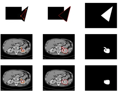
Figure 1: Results for Rada-Chen [28], for three test problems (given by rows 1-3). From left to right: initialization (with user input setA), nal contour, object selected
the successful results of Rada-Chen [28], whilst both models are sensitive to initialization, as evident in row 3 of each gure. The nature of the failure in each case is due to nding a local minimum, as is possible for the nonconvex formulation. This is evident from the fact that the user input set,A, is the same for rows 2 and 3 whilst the initializations are dierent, and one case fails where as the other succeeds. This provides the motivation for convexifying the energy in the DSS case, as this cause of failure is removed.
5.2 Test Set 2 demonstration of independence of initialization of CDSS In Fig. 3 results for CDSS are presented for three examples. The function is initialized as the given image, with successful segmentation in each case. In Figs. 4 and 5 the same object is selected, with dierent user input for each. The solution (ground truth) is given by an ideal user input set, A∗, which is the shape of the target object and would require n
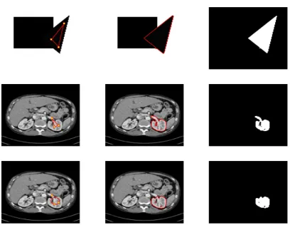
Figure 2: Results for DSS, for three test problems (given by rows 1-3). From left to right: initialization (with user input set A), nal contour, object selected
input, A4 from Fig. 4 and A5 from Figure 5. WhilstA5 is close to the boundary of the target (and closer to the ideal user input,A∗),A4 is a more interior selection. These produce slightly dierent results, but both are acceptable. This demonstrates that even with a simple user input far from the ideal, such as A4, we get an acceptable result. A more appropriate user input (i.e. closer to the ideal), such as A5, produces a better result, but still only requires three points. One observes that the initializations were deliberately chosen to be not within the object intended (which would fail with all other nonconvex models) and yet CDSS "knows" where the intended object is and nds it correctly. These examples demonstrate the robustness of the model; successful segmentation is possible for a wide range of user input.
5.3 Test Set 3 demonstration of eectiveness of the new AOS algorithm In Fig. 6 the residual is shown forAOS0for two dierent time steps;τ = 10−2andτ = 10−3. It demonstrates that for a stable convergence, the time step is limited toτ = 10−3. In Fig. 7 the
residual is shown forAOS1 for τ = 10−2 for two dierent choices of the restriction parameter;
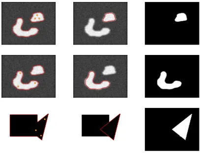
Figure 3: Results for CDSS, for three test problems (given by rows 1-3). From left to right: initialization (with user input set A), nal contour, object selected.
convergence for a higher time step than original AOS (AOS0), for an appropriate selection ofς. In Fig. 8 the residual is shown forAOS1 forτ = 10−1for two dierent choices of the restriction parameter; ς = 0.1 and ς = 0.5. It demonstrates that the improved AOS (AOS1) can achieve stable convergence for higher time steps, depending on the selection of ς. We have found that
the fastest stable convergence is for τ = 10−2, ς = 0.1.
In Fig. 9 the residual is shown forAOS2 forτ = 1for two dierent choices of the restriction parameter; ς = 0.1 and ς = 0.5. It demonstrates that AOS2 can achieve stable convergence for a higher time step than AOS0 and AOS1, for an appropriate selection of ς, i.e. ˜b = b. This scheme (AOS2) complies with the discrete scale space conditions [29] for ς = 0.5, and has stable convergence for large time steps. It can be seen as a variable time step, given by ˜τ
(4.17), dependent on the contribution of the penalty term.
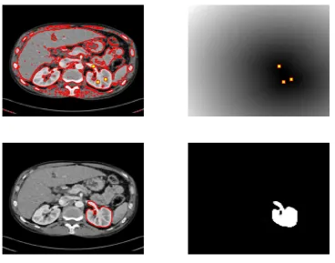
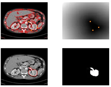
Figure 4: User input set 1 for CDSS. From left to right, top to bottom: initialization, Pd
function (with user input setA4), nal contour, object selected.
applicable to convex segmentation; and Yuan et al. [30] introduced a max ow based algorithm for binary labelling problems. These methods would further improve the results for CDSS, in terms of computational eciency.
6 Conclusions
Figure 5: User input set 2 for CDSS. From left to right, top to bottom: initialization, Pd
function (with user input setA5), nal contour, object selected.
References
[1] N. Badshah and K. Chen. Image selective segmentation under geometrical constraints using an active contour approach. Commun. Comput. Phys., 7(4):759778, 2009.
[2] N. Badshah, K. Chen, H. Ali, and G. Murtaza. Coecient of variation based image selective segmentation model using active contours. East Asian Journal on Applied Mathematics, 2:150169, 2012.
[3] E. Bae, J. Yuan, and X. C. Tai. Global minimization for continuous multiphase partitioning problems using a dual approach. Int. J. Computer Vision, 92:112129, 2011.
[4] X. Bresson, S. Esedoglu, P. Vandergheynst, J. P. Thiran, and S. Osher. Fast global minimization of the active contour/snake model. J. Math. Imaging Vis., 28:151167, 2007. [5] V. Caselles, R. Kimmel, and G. Sapiro. Geodesic active contours. International Journal
of Computer Vision, 22(1):6179, 1997.
Figure 6: Results forAOS0 for CDSS. Row 1 is forτ = 10−2, row 2 is forτ = 10−3. From left to right: nal contour and residual foru (with number of iterations).
[7] A. Chambolle and T. Pock. A rst-order primal-dual algorithm for convex problems with applications to imaging. Journal of Mathematical Imaging and Vision, 40:120145, 2011. [8] T. F. Chan, S. Esedoglu, and M. Nikilova. Algorithms for nding global minimizers
of image segmentationand denoising models. SIAM Journal on Applied Mathematics, 66:19321648, 2006.
[9] T. F. Chan and J. H. Shen. Image Processing and Analysis - Variational, PDE, Wavelet, and Stochastic Methods. SIAM Publications, Philadelphia, USA, 2005.
[10] T. F. Chan and L. Vese. Active contours without edges. IEEE Transactions on Image Processing, 10(2):266277, 2001.
[11] E. Giusti. Minimal Surfaces and Functions of Bounded Variation. Birkhauser Boston, 1984.
Figure 7: Results for AOS1, τ = 10−2 for CDSS. Row 1 is for ς = 0.01, row 2 is for ς = 0.1. From left to right: nal contour and residual foru (with number of iterations).
[13] C. Gout and C. Le Guyader. Geodesic active contour under geometrical conditions theory and 3d applications. Numerical Algorithms, 48:105133, 2008.
[14] C. Gout, C. Le Guyader, and L. Vese. Segmentation under geometrical conditions with geodesic active contour and interpolation using level set method. Numerical Algorithms, 39:155173, 2005.
[15] Y. Gu, L. L. Wang, and X. C. Tai. A direct approach towards global minimization for multiphase labeling and segmentation problems. IEEE Transactions on Image Processing, 21:2399 2411, 2012.
[16] J. B. Hiriart-Urruty and C. Lemarecheal. Convex Analysis and Minimization Algorithms. I. Fundamentals. Grundlehren Math. Wiss. 305. Springer-Verlag, New York, 1993.
Figure 8: Results for AOS1, τ = 10−1 for CDSS. Row 1 is for ς = 0.1, row 2 is for ς = 0.5. From left to right: nal contour and residual foru (with number of iterations).
[18] J. Lellmann, F. Becker, and C. Schnörr. Convex optimization for multi-class image labeling with a novel family of total variation based regularizers. In IEEE International Conference on Computer Vision (ICCV), 2009.
[19] C. Li, C. Xu, C. Gui, and M. D. Fox. Level set evolution without re-initialization: A new variational formulation. IEEE Computer Society Conference on Computer Vision and Pattern Recognition, 1:430436, 2005.
[20] T. Lu, P. Neittaanmaki, and X. C. Tai. A parallel splitting-up method for partial dieren-tial equations and its application to navier-stokes equations. RAIRO Math. Mod. Numer. Anal., 26(6):673708, 1992.
[21] A. Mitiche and I. Ben-Ayed. Variational and Level Set Methods in Image Segmentation. Springer Topics in Signal Processing. Springer, 2010.
Figure 9: Results for AOS2, τ = 1 for CDSS. Row 1 is forς = 0.1, row 2 is for ς = 0.5. From left to right: nal contour and residual for u(with number of iterations).
[23] E. Mylona, M. Savelonas, and D. Maroulis. Automated adjustment of region-based active contour parameters using local image geometry. IEEE Transactions on cybernetics, 2014. to appear.
[24] M. Ng, G. Qiu, and A. Yip. Numerical methods for interactive multiple class image segmentation problems. Int. J. Imaging Systems and Technology, 20:191201, 2010. [25] T. Nguyen, J. Cai, J. Zhang, and J. Zheng. Robust interactive image segmentation using
convex active contours. IEEE Transactions on Image Processing, 21:37343743, 2012. [26] S. Osher and J. Sethian. Fronts propagating with curvature-dependent speed: algorithms
based on Hamilton-Jacobi formulations. J. Computational Physics, 79(1):1249, 1988. [27] L. Rada and K. Chen. A new variational model with dual level set functions for selective
segmentation. Commun. Comput. Physics, 12(1):261283, 2012.
[29] J. Weickert, B. M. ter Haar Romeny, and Max A. Viergever. Ecient and reliable schemes for nonlinear diusion ltering. IEEE Transactions on Image Processing, 7:398410, 1998. [30] J. Yuan, E. Bae, X.C. Tai, and Y. Boykov. A spatially continuous max-ow and min-cut framework for binary labeling problems. Numerische Mathematik, 126(3):559587, 2014. [31] J. P. Zhang, K. Chen, and B. Yu. A 3D multigrid algorithm for the Chan-Vese model of
variational image segmentation. Int. Journal of Computer Math., 89:160189, 2012. [32] Y. L. Zheng and K. Chen. A hierarchical algorithm for multiphase texture image