Introduction to Real Analysis, Volume I
Typeset in LATEX.
Copyright c2009–2019 Jiˇrí Lebl
This work is dual licensed under the Creative Commons Attribution-Noncommercial-Share Alike 4.0 International License and the Creative Commons Attribution-Share Alike 4.0 International License. To view a copy of these licenses, visithttps://creativecommons.org/licenses/ by-nc-sa/4.0/ or https://creativecommons.org/licenses/by-sa/4.0/ or send a letter to Creative Commons PO Box 1866, Mountain View, CA 94042, USA.
You can use, print, duplicate, share this book as much as you want. You can base your own notes on it and reuse parts if you keep the license the same. You can assume the license is either the CC-BY-NC-SA or CC-BY-SA, whichever is compatible with what you wish to do, your derivative works must use at least one of the licenses. Derivative works must be prominently marked as such.
During the writing of these notes, the author was in part supported by NSF grants DMS-0900885 and DMS-1362337.
The date is the main identifier of version. The major version / edition number is raised only if there have been substantial changes. Each volume has its own version number. Edition number started at 4, that is, version 4.0, as it was not kept track of before.
Seehttps://www.jirka.org/ra/for more information (including contact information, possible updates and errata).
Introduction 5
0.1 About this book . . . 5
0.2 About analysis . . . 7
0.3 Basic set theory . . . 8
1 Real Numbers 21 1.1 Basic properties . . . 21
1.2 The set of real numbers . . . 26
1.3 Absolute value and bounded functions . . . 33
1.4 Intervals and the size ofR . . . 38
1.5 Decimal representation of the reals . . . 41
2 Sequences and Series 47 2.1 Sequences and limits . . . 47
2.2 Facts about limits of sequences . . . 56
2.3 Limit superior, limit inferior, and Bolzano–Weierstrass . . . 67
2.4 Cauchy sequences . . . 77
2.5 Series . . . 80
2.6 More on series. . . 92
3 Continuous Functions 103 3.1 Limits of functions . . . 103
3.2 Continuous functions . . . 111
3.3 Min-max and intermediate value theorems . . . 118
3.4 Uniform continuity . . . 125
3.5 Limits at infinity . . . 131
3.6 Monotone functions and continuity . . . 135
4 The Derivative 141 4.1 The derivative . . . 141
4.2 Mean value theorem. . . 147
4.3 Taylor’s theorem . . . 155
5 The Riemann Integral 163
5.1 The Riemann integral . . . 163
5.2 Properties of the integral . . . 172
5.3 Fundamental theorem of calculus . . . 180
5.4 The logarithm and the exponential . . . 186
5.5 Improper integrals. . . 192
6 Sequences of Functions 205 6.1 Pointwise and uniform convergence . . . 205
6.2 Interchange of limits . . . 212
6.3 Picard’s theorem . . . 223
7 Metric Spaces 229 7.1 Metric spaces . . . 229
7.2 Open and closed sets . . . 237
7.3 Sequences and convergence. . . 246
7.4 Completeness and compactness. . . 251
7.5 Continuous functions . . . 259
7.6 Fixed point theorem and Picard’s theorem again . . . 267
Further Reading 271
Index 273
0.1
About this book
This first volume is a one semester course in basic analysis. Together with the second volume it is a year-long course. It started its life as my lecture notes for teaching Math 444 at the University of Illinois at Urbana-Champaign (UIUC) in Fall semester 2009. Later I added the metric space chapter to teach Math 521 at University of Wisconsin–Madison (UW). Volume II was added to teach Math 4143/4153 at Oklahoma State University (OSU). A prerequisite for these courses is usually a basic proof course, using for example [H], [F], or [DW].
It should be possible to use the book for both a basic course for students who do not necessarily wish to go to graduate school (such as UIUC 444), but also as a more advanced one-semester course that also covers topics such as metric spaces (such as UW 521). Here are my suggestions for what to cover in a semester course. For a slower course such as UIUC 444:
§0.3, §1.1–§1.4, §2.1–§2.5, §3.1–§3.4, §4.1–§4.2, §5.1–§5.3, §6.1–§6.3
For a more rigorous course covering metric spaces that runs quite a bit faster (such as UW 521): §0.3, §1.1–§1.4, §2.1–§2.5, §3.1–§3.4, §4.1–§4.2, §5.1–§5.3, §6.1–§6.2, §7.1–§7.6
It should also be possible to run a faster course without metric spaces covering all sections of chapters 0 through 6. The approximate number of lectures given in the section notes through chapter 6 are a very rough estimate and were designed for the slower course. The first few chapters of the book can be used in an introductory proofs course as is for example done at Iowa State University Math 201, where this book is used in conjunction with Hammack’s Book of Proof [H].
With volume II one can run a year-long course that also covers multivariable topics. It may make sense in this case to cover most of the first volume in the first semester while leaving metric spaces for the beginning of the second semester.
The book normally used for the class at UIUC is Bartle and Sherbert, Introduction to Real Analysis third edition [BS]. The structure of the beginning of the book somewhat follows the standard syllabus of UIUC Math 444 and therefore has some similarities with [BS]. A major difference is that we define the Riemann integral using Darboux sums and not tagged partitions. The Darboux approach is far more appropriate for a course of this level.
Other excellent books exist. My favorite is Rudin’s excellent Principles of Mathematical Analysis[R2] or, as it is commonly and lovingly called,baby Rudin(to distinguish it from his other great analysis textbook, big Rudin). I took a lot of inspiration and ideas from Rudin. However, Rudin is a bit more advanced and ambitious than this present course. For those that wish to continue mathematics, Rudin is a fine investment. An inexpensive and somewhat simpler alternative to Rudin is Rosenlicht’sIntroduction to Analysis[R1]. There is also the freely downloadableIntroduction to Real Analysisby William Trench [T].
A note about the style of some of the proofs: Many proofs traditionally done by contradiction, I prefer to do by a direct proof or by contrapositive. While the book does include proofs by contradiction, I only do so when the contrapositive statement seemed too awkward, or when contradiction follows rather quickly. In my opinion, contradiction is more likely to get beginning students into trouble, as we are talking about objects that do not exist.
I try to avoid unnecessary formalism where it is unhelpful. Furthermore, the proofs and the language get slightly less formal as we progress through the book, as more and more details are left out to avoid clutter.
As a general rule, I use :=instead of=to define an object rather than to simply show equality. I use this symbol rather more liberally than is usual for emphasis. I use it even when the context is “local,” that is, I may simply define a function f(x):=x2for a single exercise or example.
0.2
About analysis
Analysis is the branch of mathematics that deals with inequalities and limits. The present course deals with the most basic concepts in analysis. The goal of the course is to acquaint the reader with rigorous proofs in analysis and also to set a firm foundation for calculus of one variable (and several variables if volume II is also considered).
Calculus has prepared you, the student, for using mathematics without telling you why what you learned is true. To use, or teach, mathematics effectively, you cannot simply knowwhatis true, you must knowwhyit is true. This course shows youwhycalculus is true. It is here to give you a good understanding of the concept of a limit, the derivative, and the integral.
Let us use an analogy. An auto mechanic that has learned to change the oil, fix broken headlights, and charge the battery, will only be able to do those simple tasks. He will be unable to work independently to diagnose and fix problems. A high school teacher that does not understand the definition of the Riemann integral or the derivative may not be able to properly answer all the students’ questions. To this day I remember several nonsensical statements I heard from my calculus teacher in high school, who simply did not understand the concept of the limit, though he could “do” the problems in in the textbook.
We start with a discussion of the real number system, most importantly its completeness property, which is the basis for all that comes after. We then discuss the simplest form of a limit, the limit of a sequence. Afterwards, we study functions of one variable, continuity, and the derivative. Next, we define the Riemann integral and prove the fundamental theorem of calculus. We discuss sequences of functions and the interchange of limits. Finally, we give an introduction to metric spaces.
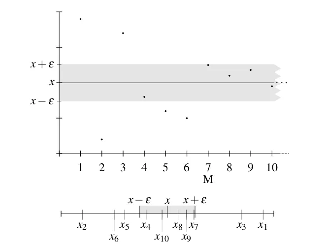
Let us give the most important difference between analysis and algebra. In algebra, we prove equalities directly; we prove that an object, a number perhaps, is equal to another object. In analysis, we usually prove inequalities, and we prove those inequalities by estimating. To illustrate the point, consider the following statement.
Let x be a real number. If x<ε is true for all real numbersε >0, then x≤0.
This statement is the general idea of what we do in analysis. Suppose next we really wish to prove the equalityx=0. In analysis, we prove two inequalities: x≤0 andx≥0. To prove the inequalityx≤0, we provex<εfor all positiveε. To prove the inequalityx≥0, we provex>−ε
for all positiveε.
The termreal analysisis a little bit of a misnomer. I prefer to use simplyanalysis. The other type of analysis,complex analysis, really builds up on the present material, rather than being distinct. Furthermore, a more advanced course on real analysis would talk about complex numbers often. I suspect the nomenclature is historical baggage.
0.3
Basic set theory
Note: 1–3 lectures (some material can be skipped, covered lightly, or left as reading)
Before we start talking about analysis, we need to fix some language. Modern∗analysis uses the language of sets, and therefore that is where we start. We talk about sets in a rather informal way, using the so-called “naïve set theory.” Do not worry, that is what majority of mathematicians use, and it is hard to get into trouble. The reader has hopefully seen the very basics of set theory and proof writing before, and this section should be a quick refresher.
0.3.1
Sets
Definition 0.3.1. Asetis a collection of objects calledelementsormembers. A set with no objects is called theempty setand is denoted by /0 (or sometimes by{}).
Think of a set as a club with a certain membership. For example, the students who play chess are members of the chess club. However, do not take the analogy too far. A set is only defined by the members that form the set; two sets that have the same members are the same set.
Most of the time we will consider sets of numbers. For example, the set
S:={0,1,2}
is the set containing the three elements 0, 1, and 2. By “:=”, we mean we are defining whatSis, rather than just showing equality. We write
1∈S
to denote that the number 1 belongs to the setS. That is, 1 is a member ofS. At times we want to say that two elements are in a setS, so we write “1,2∈S” as a shorthand for “1∈Sand 2∈S.”
Similarly, we write
7∈/S
to denote that the number 7 is not inS. That is, 7 is not a member ofS.
The elements of all sets under consideration come from some set we call the universe. For simplicity, we often consider the universe to be the set that contains only the elements we are interested in. The universe is generally understood from context and is not explicitly mentioned. In this course, our universe will most often be the set of real numbers.
While the elements of a set are often numbers, other objects, such as other sets, can be elements of a set. A set may also contain some of the same elements as another set. For example,
T :={0,2}
contains the numbers 0 and 2. In this case all elements ofT also belong toS. We writeT ⊂S. See Figure 1for a diagram.
T S
0 2
1 7
Figure 1:A diagram of the example setsSand its subsetT.
Definition 0.3.2.
(i) A setAis asubsetof a setBifx∈Aimpliesx∈B, and we writeA⊂B. That is, all members ofAare also members ofB. At times we writeB⊃Ato mean the same thing.
(ii) Two setsAandBareequalifA⊂Band B⊂A. We writeA=B. That is,AandBcontain exactly the same elements. If it is not true thatAandBare equal, then we writeA6=B. (iii) A setAis aproper subsetofBifA⊂BandA6=B. We writeA(B.
For example, forSandT defined aboveT ⊂S, butT =6 S. SoT is a proper subset ofS. IfA=B, thenAandBare simply two names for the same exact set. Let us mention theset building notation,
x∈A:P(x) .
This notation refers to a subset of the setAcontaining all elements ofAthat satisfy the property P(x). For example, usingS={0,1,2}as above,{x∈S:x6=2}is the set{0,1}. The notation is
sometimes abbreviated,Ais not mentioned when understood from context. Furthermore,x∈Ais sometimes replaced with a formula to make the notation easier to read.
Example 0.3.3: The following are sets including the standard notations. (i) The set ofnatural numbers,N:={1,2,3, . . .}.
(ii) The set ofintegers,Z:={0,−1,1,−2,2, . . .}.
(iii) The set ofrational numbers,Q:={mn :m,n∈Zandn6=0}.
(iv) The set of even natural numbers,{2m:m∈N}.
(v) The set of real numbers,R.
Note thatN⊂Z⊂Q⊂R.
There are many operations we want to do with sets.
Definition 0.3.4.
(i) Aunionof two setsAandBis defined as
A∪B:={x:x∈Aorx∈B}.
(ii) Anintersectionof two setsAandBis defined as
(iii) Acomplement of B relative to A(orset-theoretic differenceofAandB) is defined as A\B:={x:x∈Aandx∈/B}.
(iv) We saycomplementofBand writeBcinstead ofA\Bif the setAis either the entire universe or is the obvious set containingB, and is understood from context.
(v) We say setsAandBaredisjointifA∩B=/0.
The notationBc may be a little vague at this point. If the setBis a subset of the real numbersR,
thenBcmeans
R\B. IfBis naturally a subset of the natural numbers, thenBcisN\B. If ambiguity
can arise, we use the set difference notationA\B.
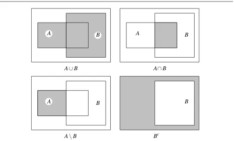
A∪B
A\B Bc
A∩B
B
A B A B
[image:10.612.77.542.244.525.2]B A
Figure 2:Venn diagrams of set operations, the result of the operation is shaded.
We illustrate the operations on theVenn diagramsin Figure 2. Let us now establish one of most basic theorems about sets and logic.
Theorem 0.3.5(DeMorgan). Let A,B,C be sets. Then
(B∪C)c=Bc∩Cc,
(B∩C)c=Bc∪Cc,
or, more generally,
A\(B∪C) = (A\B)∩(A\C),
Proof. The first statement is proved by the second statement if we assume the setAis our “universe.” Let us proveA\(B∪C) = (A\B)∩(A\C). Remember the definition of equality of sets. First, we must show that ifx∈A\(B∪C), thenx∈(A\B)∩(A\C). Second, we must also show that if x∈(A\B)∩(A\C), thenx∈A\(B∪C).
So let us assumex∈A\(B∪C). Thenxis inA, but not inBnorC. Hencexis inAand not in B, that is,x∈A\B. Similarlyx∈A\C. Thusx∈(A\B)∩(A\C).
On the other hand supposex∈(A\B)∩(A\C). In particular,x∈(A\B), sox∈Aandx∈/B.
Also asx∈(A\C), thenx∈/C. Hencex∈A\(B∪C).
The proof of the other equality is left as an exercise.
The result above we called aTheorem, while most results we call aProposition, and a few we call aLemma(a result leading to another result) orCorollary(a quick consequence of the preceding result). Do not read too much into the naming. Some of it is traditional, some of it is stylistic choice. It is not necessarily true that aTheoremis always “more important” than aPropositionor aLemma. We will also need to intersect or union several sets at once. If there are only finitely many, then we simply apply the union or intersection operation several times. However, suppose we have an infinite collection of sets (a set of sets){A1,A2,A3, . . .}. We define
∞ [
n=1
An:={x:x∈Anfor somen∈N},
∞ \
n=1
An:={x:x∈Anfor alln∈N}.
We can also have sets indexed by two integers. For example, we can have the set of sets {A1,1,A1,2,A2,1,A1,3,A2,2,A3,1, . . .}. Then we write
∞ [
n=1 ∞ [
m=1
An,m= ∞ [
n=1 ∞ [
m=1 An,m
!
.
And similarly with intersections.
It is not hard to see that we can take the unions in any order. However, switching the order of unions and intersections is not generally permitted without proof. For example:
∞ [
n=1 ∞ \
m=1
{k∈N:mk<n}=
∞ [
n=1 /0= /0.
However,
∞ \
m=1
∞ [
n=1
{k∈N:mk<n}=
∞ \
m=1
N=N.
Sometimes, the index set is not the natural numbers. In this case we need a more general notation. SupposeIis some set and for eachλ ∈I, we have a setAλ. Then we define
[
λ∈I
Aλ :={x:x∈Aλ for someλ ∈I},
\
λ∈I
0.3.2
Induction
When a statement includes an arbitrary natural number, a common method of proof is the principle of induction. We start with the set of natural numbersN={1,2,3, . . .}, and we give them their
natural ordering, that is, 1<2<3<4<···. ByS⊂Nhaving aleast element, we mean that there
exists anx∈S, such that for everyy∈S, we havex≤y.
The natural numbersNordered in the natural way possess the so-calledwell ordering property.
We take this property as an axiom; we simply assume it is true.
Well ordering property ofN. Every nonempty subset ofNhas a least (smallest) element.
Theprinciple of inductionis the following theorem, which is equivalent to the well ordering property of the natural numbers.
Theorem 0.3.6(Principle of induction). Let P(n)be a statement depending on a natural number n. Suppose that
(i) (basis statement)P(1)is true,
(ii) (induction step)if P(n)is true, then P(n+1)is true. Then P(n)is true for all n∈N.
Proof. SupposeSis the set of natural numbersmfor whichP(m)is not true. SupposeSis nonempty. Then S has a least element by the well ordering property. Let us call mthe least element of S. We know 1∈/Sby assumption. Thereforem>1 andm−1 is a natural number as well. Sincem is the least element of S, we know that P(m−1) is true. But by the induction step we see that P(m−1+1) =P(m)is true, contradicting the statement thatm∈S. ThereforeSis empty andP(n) is true for alln∈N.
Sometimes it is convenient to start at a different number than 1, but all that changes is the labeling. The assumption thatP(n)is true in “ifP(n)is true, thenP(n+1)is true” is usually called theinduction hypothesis.
Example 0.3.7: Let us prove that for alln∈N,
2n−1≤n! (recalln!=1·2·3···n).
We letP(n)be the statement that 2n−1≤n! is true. By plugging inn=1, we see thatP(1)is true. SupposeP(n)is true. That is, suppose 2n−1≤n! holds. Multiply both sides by 2 to obtain
2n≤2(n!).
As 2≤(n+1)whenn∈N, we have 2(n!)≤(n+1)(n!) = (n+1)!. That is,
2n≤2(n!)≤(n+1)!,
and henceP(n+1)is true. By the principle of induction, we see that P(n) is true for alln, and hence 2n−1≤n! is true for alln∈
Example 0.3.8: We claim that for allc6=1,
1+c+c2+···+cn=1−c
n+1 1−c .
Proof: It is easy to check that the equation holds withn=1. Suppose it is true forn. Then
1+c+c2+···+cn+cn+1= (1+c+c2+···+cn) +cn+1
= 1−c
n+1 1−c +c
n+1
= 1−c
n+1+ (1−c)cn+1 1−c
= 1−c
n+2 1−c .
Sometimes, it is easier to use in the inductive step thatP(k)is true for allk=1,2, . . . ,n, not just
fork=n. This principle is calledstrong inductionand is equivalent to the normal induction above. The proof that equivalence is left as an exercise.
Theorem 0.3.9 (Principle of strong induction). Let P(n)be a statement depending on a natural number n. Suppose that
(i) (basis statement)P(1)is true,
(ii) (induction step)if P(k)is true for all k=1,2, . . . ,n, then P(n+1)is true. Then P(n)is true for all n∈N.
0.3.3
Functions
Informally, a set-theoretic function f taking a set Ato a set B is a mapping that to each x∈A assigns a uniquey∈B. We write f: A→B. For example, we define a function f: S→T taking S={0,1,2} toT ={0,2} by assigning f(0):=2, f(1):=2, and f(2):=0. That is, a function f: A→Bis a black box, into which we stick an element ofAand the function spits out an element ofB. Sometimes f is called amappingor amap, and we say f maps A to B.
Often, functions are defined by some sort of formula, however, you should really think of a function as just a very big table of values. The subtle issue here is that a single function can have several formulas, all giving the same function. Also, for many functions, there is no formula that expresses its values.
To define a function rigorously, first let us define the Cartesian product.
Definition 0.3.10. LetAandBbe sets. TheCartesian productis the set of tuples defined as A×B:={(x,y):x∈A,y∈B}.
Definition 0.3.11. Afunction f: A→Bis a subset f ofA×Bsuch that for eachx∈A, there is a unique(x,y)∈ f. We then write f(x) =y. Sometimes the set f is called thegraphof the function
rather than the function itself.
The setAis called thedomainof f (and sometimes confusingly denotedD(f)). The set
R(f):={y∈B: there exists anxsuch that f(x) =y}
is called therangeof f.
It is possible that the rangeR(f)is a proper subset ofB, while the domain of f is always equal toA. We usually assume that the domain of f is nonempty.
Example 0.3.12: From calculus, you are most familiar with functions taking real numbers to real numbers. However, you saw some other types of functions as well. For example, the derivative is a function mapping the set of differentiable functions to the set of all functions. Another example is the Laplace transform, which also takes functions to functions. Yet another example is the function that takes a continuous functiongdefined on the interval[0,1]and returns the numberR1
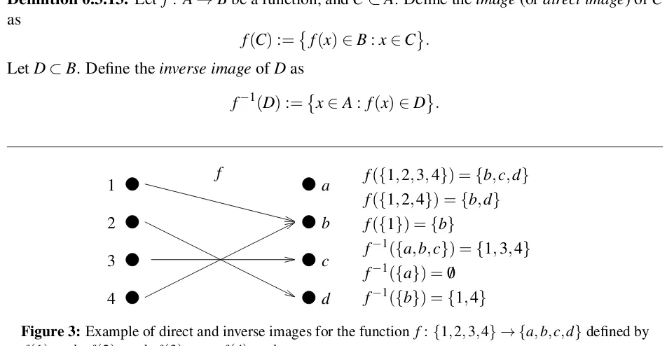
0 g(x)dx. Definition 0.3.13. Let f: A→Bbe a function, andC⊂A. Define theimage(ordirect image) ofC as
f(C):=
f(x)∈B:x∈C .
LetD⊂B. Define theinverse imageofDas
f−1(D):=
x∈A: f(x)∈D .
a 1
2
3
4
b
c
d
f f({1,2,3,4}) ={b,c,d} f({1,2,4}) ={b,d}
f({1}) ={b}
f−1({a,b,c}) ={1,3,4} f−1({a}) = /0
[image:14.612.67.543.325.572.2]f−1({b}) ={1,4}
Figure 3:Example of direct and inverse images for the function f:{1,2,3,4} → {a,b,c,d}defined by f(1):=b, f(2):=d, f(3):=c, f(4):=b.
Example 0.3.14: Define the function f: R→R by f(x) :=sin(πx). Then f([0,1/2]) = [0,1],
f−1({0}) =
Z, etc.
Proposition 0.3.15. Let f: A→B. Let C,D be subsets of B. Then
f−1(C∪D) = f−1(C)∪ f−1(D), f−1(C∩D) = f−1(C)∩ f−1(D), f−1(Cc) = f−1(C)c
Read the last line of the proposition as f−1(B\C) =A\f−1(C).
Proof. Let us start with the union. Supposex∈ f−1(C∪D). That meansxmaps toCorD. Thus f−1(C∪D)⊂ f−1(C)∪f−1(D). Conversely ifx∈ f−1(C), thenx∈ f−1(C∪D). Similarly for x∈ f−1(D). Hence f−1(C∪D)⊃ f−1(C)∪f−1(D), and we have equality.
The rest of the proof is left as an exercise.
The proposition does not hold for direct images. We do have the following weaker result.
Proposition 0.3.16. Let f: A→B. Let C,D be subsets of A. Then
f(C∪D) = f(C)∪f(D),
f(C∩D)⊂ f(C)∩f(D).
The proof is left as an exercise.
Definition 0.3.17. Let f: A→Bbe a function. The function f is said to beinjectiveorone-to-one if f(x1) = f(x2)impliesx1=x2. In other words, for ally∈Bthe set f−1({y})is empty or consists of a single element. We call such an f aninjection.
The function f is said to besurjectiveorontoif f(A) =B. We call such an f asurjection. A function f that is both an injection and a surjection is said to bebijective, and we say f is a bijection.
When f: A→B is a bijection, then f−1({y}) is always a unique element of A, and we can consider f−1as a function f−1: B→A. In this case, we call f−1the inverse functionof f. For example, for the bijection f: R→Rdefined by f(x):=x3we have f−1(x) =√3x.
A final piece of notation for functions that we need is thecomposition of functions.
Definition 0.3.18. Let f: A→B,g: B→C. The functiong◦f:A→Cis defined as (g◦f)(x):=g f(x)
.
0.3.4
Relations and equivalence classes
We often compare two objects in some way. We say 1<2 for natural numbers, or1/2=2/4for rational numbers, or{a,c} ⊂ {a,b,c}for sets. The ‘<’, ‘=’, and ‘⊂’ are examples of relations.
Definition 0.3.19. Given a setA, abinary relationon Ais a subsetR ⊂A×A, which are those pairs where the relation is said to hold. Instead of(a,b)∈R, we writeaRb.
Example 0.3.20: TakeA:={1,2,3}.
Consider the relation ‘<’. The corresponding set of pairs is
(1,2),(1,3),(2,3) . So 1<2
holds as(1,2)is in the corresponding set of pairs, but 3<1 does not hold as(3,1)is not in the set. Similarly, the relation ‘=’ is defined by the set of pairs
(1,1),(2,2),(3,3) . Any subset ofA×Ais a relation. Let us define the relation † via
Definition 0.3.21. LetR be a relation on a setA. ThenR is said to be (i) reflexiveifaRafor alla∈A.
(ii) symmetricifaRbimpliesbRa.
(iii) transitiveifaRbandbRcimpliesaRc.
IfR is reflexive, symmetric, and transitive, then it is said to be anequivalence relation.
Example 0.3.22: LetA:={1,2,3}as above. The relation ‘<’ is transitive, but neither reflexive nor
symmetric. The relation ‘≤’ defined by
(1,1),(1,2),(1,3),(2,2),(2,3),(3,3) is reflexive and transitive, but not symmetric. Finally, a relation ‘?’ defined by
(1,1),(1,2),(2,1),(2,2),(3,3) is an equivalence relation.
Equivalence relations are useful in that they divide a set into sets of “equivalent” elements.
Definition 0.3.23. LetAbe a set andR an equivalence relation. Anequivalence classofa∈A, often denoted by[a], is the set{x∈A:aRx}.
For example, for the relation ‘?’ above, the equivalence classes are [1] = [2] ={1,2} and
[3] ={3}.
Reflexivity guarantees thata∈[a]. Symmetry guarantees that ifb∈[a], thena∈[b]. Finally, transitivity guarantees that ifa∈[b]andb∈[c], thena∈[c]. In particular, we have the following proposition, whose proof is an exercise.
Proposition 0.3.24. IfR is an equivalence relation on a set A, then every a∈A is in exactly one equivalence class. In particular, aRb if and only[a] = [b].
Example 0.3.25: The set of rational numbers can be defined as equivalence classes of a pair of an integer and a natural number, that is elements ofZ×N. The relation is defined by(a,b)∼(c,d)
wheneverad=bc. It is left as an exercise to prove that ‘∼’ is an equivalence relation. Usually the equivalence class[(a,b)]is written asa/b.
0.3.5
Cardinality
A subtle issue in set theory and one generating a considerable amount of confusion among students is that of cardinality, or “size” of sets. The concept of cardinality is important in modern mathematics in general and in analysis in particular. In this section, we will see the first really unexpected theorem.
Definition 0.3.26. LetAandBbe sets. We sayAandBhave the samecardinalitywhen there exists a bijection f: A→B. We denote by|A|the equivalence class of all sets with the same cardinality asAand we simply call|A|the cardinality ofA.
For example {1,2,3}has the same cardinality as {a,b,c}by defining a bijection f(1):=a, f(2):=b, f(3):=c. Clearly the bijection is not unique.
Definition 0.3.27. SupposeAhas the same cardinality as{1,2,3, . . . ,n}for somen∈N. We then
write|A|:=n. IfAis empty we write|A|:=0. In either case we say thatAisfinite. We sayAisinfiniteor “of infinite cardinality” ifAis not finite.
That the notation|A|=nis justified we leave as an exercise. That is, for each nonempty finite set A, there exists a unique natural numbernsuch that there exists a bijection fromAto{1,2,3, . . . ,n}.
We can order sets by size.
Definition 0.3.28. We write
|A| ≤ |B|
if there exists an injection fromAtoB. We write|A|=|B|ifAandBhave the same cardinality. We write|A|<|B|if|A| ≤ |B|, butAandBdo not have the same cardinality.
We state without proof that |A|=|B| have the same cardinality if and only if |A| ≤ |B| and
|B| ≤ |A|. This is the so-called Cantor–Bernstein–Schröder theorem. Furthermore, ifAandBare
any two sets, we can always write|A| ≤ |B|or|B| ≤ |A|. The issues surrounding this last statement are very subtle. As we do not require either of these two statements, we omit proofs.
The truly interesting cases of cardinality are infinite sets. We will distinguish two types of infinite cardinality.
Definition 0.3.29. If|A|=|N|, then Ais said to becountably infinite. IfAis finite or countably
infinite, then we sayAiscountable. IfAis not countable, thenAis said to beuncountable.
The cardinality ofNis usually denoted asℵ0(read as aleph-naught)∗.
Example 0.3.30: The set of even natural numbers has the same cardinality asN. Proof: LetE⊂N be the set of even natural numbers. Givenk∈E, writek=2nfor somen∈N. Then f(n):=2n
defines a bijection f: N→E.
In fact, let us mention without proof the following characterization of infinite sets: A set is infinite if and only if it is in one-to-one correspondence with a proper subset of itself.
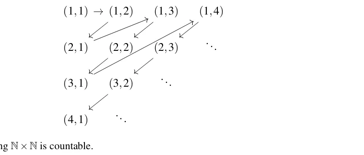
Example 0.3.31: N×Nis a countably infinite set. Proof: Arrange the elements ofN×Nas follows (1,1),(1,2),(2,1),(1,3),(2,2),(3,1), . . . . That is, always write down first all the elements whose two entries sum tok, then write down all the elements whose entries sum tok+1 and so on. Define a bijection withNby letting 1 go to(1,1), 2 go to(1,2), and so on. See Figure 4.
Example 0.3.32: The set of rational numbers is countable. Proof: (informal) Follow the same procedure as in the previous example, writing1/1,1/2,2/1, etc. However, leave out any fraction (such as2/2) that has already appeared. So the list would continue:1/3,3/1,1/4,2/3, etc.
For completeness, we mention the following statements from the exercises. If A⊂B and B is countable, then A is countable. The contrapositive of the statement is that ifAis uncountable, then Bis uncountable. As a consequence if|A|<|N|thenAis finite. Similarly, ifBis finite andA⊂B,
thenAis finite.
∗For the fans of the TV showFuturama, there is a movie theater in one episode called anℵ
(1,1) (1,2) (1,3) (1,4)
(2,1) (2,2) (2,3) ...
(3,1) (3,2) ...
[image:18.612.158.533.94.254.2](4,1) ...
Figure 4:ShowingN×Nis countable.
We give the first truly striking result. First, we need a notation for the set of all subsets of a set.
Definition 0.3.33. Thepower setof a setA, denoted byP(A), is the set of all subsets ofA. For example, if A:={1,2}, then P(A) =
/0,{1},{2},{1,2} . In particular, |A|=2 and |P(A)|=4=22. In general, for a finite setAof cardinalityn, the cardinality ofP(A)is 2n. This fact is left as an exercise. Hence, for a finite setA, the cardinality ofP(A)is strictly larger than the cardinality ofA. What is an unexpected and striking fact is that this statement is still true for infinite sets.
Theorem 0.3.34 (Cantor∗). |A|<|P(A)|. In particular, there exists no surjection from A onto
P(A).
Proof. There exists an injection f: A→P(A). For any x∈A, define f(x):={x}. Therefore |A| ≤ |P(A)|.
To finish the proof, we must show that no function g: A→P(A)is a surjection. Suppose g: A→P(A)is a function. So forx∈A,g(x)is a subset ofA. Define the set
B:=
x∈A:x∈/g(x) .
We claim thatBis not in the range ofgand hencegis not a surjection. Suppose there exists anx0 such thatg(x0) =B. Eitherx0∈Borx0∈/B. Ifx0∈B, thenx0∈/g(x0) =B, which is a contradiction. If x0∈/ B, then x0∈g(x0) =B, which is again a contradiction. Thus such an x0 does not exist. Therefore,Bis not in the range ofg, andgis not a surjection. Asgwas an arbitrary function, no surjection exists.
One particular consequence of this theorem is that there do exist uncountable sets, asP(N)must
be uncountable. A related fact is that the set of real numbers (which we study in the next chapter) is uncountable. The existence of uncountable sets may seem unintuitive, and the theorem caused quite a controversy at the time it was announced. The theorem not only says that uncountable sets exist, but that there in fact exist progressively larger and larger infinite setsN,P(N),P(P(N)),
P(P(P(N))), etc.
0.3.6
Exercises
Exercise0.3.1: Show A\(B∩C) = (A\B)∪(A\C).
Exercise0.3.2: Prove that the principle of strong induction is equivalent to the standard induction. Exercise0.3.3: Finish the proof of Proposition 0.3.15.
Exercise0.3.4:
a) Prove Proposition 0.3.16.
b) Find an example for which equality of sets in f(C∩D)⊂ f(C)∩f(D)fails. That is, find an f , A, B, C,
and D such that f(C∩D)is a proper subset of f(C)∩f(D).
Exercise0.3.5(Tricky): Prove that if A is nonempty and finite, then there exists a unique n∈Nsuch that
there exists a bijection between A and{1,2,3, . . . ,n}. In other words, the notation|A|:=n is justified. Hint:
Show that if n>m, then there is no injection from{1,2,3, . . . ,n}to{1,2,3, . . . ,m}.
Exercise0.3.6: Prove:
a) A∩(B∪C) = (A∩B)∪(A∩C).
b) A∪(B∩C) = (A∪B)∩(A∪C).
Exercise0.3.7: Let A∆B denote thesymmetric difference, that is, the set of all elements that belong to either A or B, but not to both A and B.
a) Draw a Venn diagram for A∆B. b) Show A∆B= (A\B)∪(B\A).
c) Show A∆B= (A∪B)\(A∩B).
Exercise0.3.8: For each n∈N, let An:={(n+1)k:k∈N}.
a) Find A1∩A2.
b) FindS∞
n=1An.
c) FindT∞
n=1An.
Exercise0.3.9: DetermineP(S)(the power set) for each of the following: a) S=/0,
b) S={1},
c) S={1,2},
d) S={1,2,3,4}.
Exercise0.3.10: Let f:A→B and g:B→C be functions. a) Prove that if g◦f is injective, then f is injective. b) Prove that if g◦f is surjective, then g is surjective.
c) Find an explicit example where g◦f is bijective, but neither f nor g is bijective.
Exercise0.3.11: Prove by induction that n<2nfor all n∈N.
Exercise0.3.13: Prove 11·2+21·3+···+n(n1+1)=n+n1 for all n∈N.
Exercise0.3.14: Prove13+23+···+n3=n
(n+1)
2 2
for all n∈N.
Exercise0.3.15: Prove that n3+5n is divisible by6for all n∈N.
Exercise0.3.16: Find the smallest n∈Nsuch that2(n+5)2<n3and call it n0. Show that2(n+5)2<n3
for all n≥n0.
Exercise0.3.17: Find all n∈Nsuch that n2<2n.
Exercise0.3.18: Finish the proof that the principle of inductionis equivalent to the well ordering property ofN. That is, prove the well ordering property forNusing the principle of induction.
Exercise0.3.19: Give an example of a countably infinite collection of finite sets A1,A2, . . ., whose union is
not a finite set.
Exercise0.3.20: Give an example of a countably infinite collection of infinite sets A1,A2, . . ., with Aj∩Ak
being infinite for all j and k, such thatT∞
j=1Aj is nonempty and finite.
Exercise0.3.21: Suppose A⊂B and B is finite. Prove that A is finite. That is, if A is nonempty, construct a bijection of A to{1,2, . . . ,n}.
Exercise0.3.22: Prove Proposition 0.3.24. That is, prove that ifR is an equivalence relation on a set A, then every a∈A is in exactly one equivalence class. Then prove that aRb if and only if[a] = [b].
Exercise0.3.23: Prove that the relation ‘∼’ in Example 0.3.25is an equivalence relation.
Exercise0.3.24:
a) Suppose A⊂B and B is countably infinite. By constructing a bijection, show that A is countable (that is, A is empty, finite, or countably infinite).
b) Use part a) to show that if|A|<|N|, then A is finite.
Exercise0.3.25(Challenging): Suppose|N| ≤ |S|, or in other words, S contains a countably infinite subset.
Real Numbers
1.1
Basic properties
Note: 1.5 lectures
The main object we work with in analysis is the set of real numbers. As this set is so fundamental, often much time is spent on formally constructing the set of real numbers. However, we take an easier approach here and just assume that a set with the correct properties exists. We need to start with the definitions of those properties.
Definition 1.1.1. Anordered setis a setS, together with a relation<such that
(i) For anyx,y∈S, exactly one ofx<y,x=y, ory<xholds.
(ii) Ifx<yandy<z, thenx<z.
We writex≤yifx<yorx=y. We define>and≥in the obvious way.
The set of rational numbersQis an ordered set by lettingx<yif and only ify−xis a positive
rational number, that is ify−x=p/qwhere p,q∈N. Similarly,NandZare also ordered sets.
There are other ordered sets than sets of numbers. For example, the set of countries can be ordered by landmass, so India > Lichtenstein. A typical ordered set that you have used since
primary school is the dictionary. It is the ordered set of words where the order is the so-called lexicographic ordering. Such ordered sets often appear, for example, in computer science. In this book we will mostly be interested in ordered sets of numbers.
Definition 1.1.2. LetE ⊂S, whereSis an ordered set.
(i) If there exists ab∈Ssuch thatx≤bfor allx∈E, then we sayEisbounded aboveandbis anupper boundofE.
(ii) If there exists ab∈Ssuch thatx≥bfor allx∈E, then we sayE isbounded belowandbis a lower boundofE.
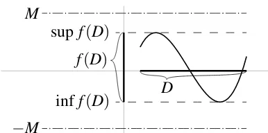
(iii) If there exists an upper boundb0ofEsuch that wheneverbis any upper bound forE we have b0≤b, thenb0is called theleast upper boundor the supremumofE. See Figure 1.1. We write
(iv) Similarly, if there exists a lower boundb0ofEsuch that wheneverbis any lower bound for Ewe haveb0≥b, thenb0is called thegreatest lower boundor theinfimumofE. We write
infE:=b0.
When a setE is both bounded above and bounded below, we say simply thatE isbounded.
upper bounds ofE
smaller bigger
least upper bound ofE
E
Figure 1.1:A setE bounded above and the least upper bound ofE.
A simple example: LetS:={a,b,c,d,e}be ordered asa<b<c<d<e, and letE:={a,c}.
Thenc,d, andeare upper bounds ofE, andcis the least upper bound or supremum ofE.
Supremum (or infimum) is automatically unique (if it exists): Ifbandb0are suprema ofE, then
b≤b0andb0≤b, because bothbandb0are the least upper bounds, sob=b0.
A supremum or infimum for E (even if they exist) need not be in E. For example, the set E:={x∈Q:x<1}has a least upper bound of 1, but 1 is not in the setEitself. On the other hand,
if we takeG:={x∈Q:x≤1}, then the least upper bound ofGis clearly also 1, and in this case
1∈G. On the other hand, the setP:={x∈Q:x≥0}has no upper bound (why?) and therefore it cannot have a least upper bound. On the other hand 0 is the greatest lower bound ofP.
Definition 1.1.3. An ordered setShas theleast-upper-bound propertyif every nonempty subset E⊂Sthat is bounded above has a least upper bound, that is supEexists inS.
Theleast-upper-bound propertyis sometimes called thecompleteness propertyor theDedekind completeness property∗. As we will note in the next section, the real numbers have this property.
Example 1.1.4: The setQof rational numbers does not have the least-upper-bound property. The subset{x∈Q:x2<2}does not have a supremum inQ. We will see later that the supremum is
√
2, which is not rational†. Supposex∈
Q such thatx2=2. Write x=m/nin lowest terms. So
(m/n)2=2 orm2=2n2. Hence,m2is divisible by 2, and somis divisible by 2. Writem=2kand
so(2k)2=2n2. Divide by 2 and note that 2k2=n2, and hence nis divisible by 2. But that is a contradiction asm/nis in lowest terms.
That Q does not have the least-upper-bound property is one of the most important reasons
why we work with Rin analysis. The setQis just fine for algebraists. But us analysts require
the least-upper-bound property to do any work. We also require our real numbers to have many algebraic properties. In particular, we require that they are a field.
∗Named after the German mathematician Julius Wilhelm Richard Dedekind(1831–1916).
†This is true for all other roots of 2, and interestingly, the fact that√k2 is never rational fork>1 implies no piano
Definition 1.1.5. A setF is called afieldif it has two operations defined on it, additionx+yand multiplicationxy, and if it satisfies the following axioms:
(A1) Ifx∈F andy∈F, thenx+y∈F.
(A2) (commutativity of addition) x+y=y+xfor allx,y∈F.
(A3) (associativity of addition)(x+y) +z=x+ (y+z)for allx,y,z∈F. (A4) There exists an element 0∈Fsuch that 0+x=xfor allx∈F.
(A5) For every elementx∈Fthere exists an element−x∈F such thatx+ (−x) =0. (M1) Ifx∈F andy∈F, thenxy∈F.
(M2) (commutativity of multiplication) xy=yxfor allx,y∈F. (M3) (associativity of multiplication)(xy)z=x(yz)for allx,y,z∈F.
(M4) There exists an element 1∈F(and 16=0) such that 1x=xfor allx∈F.
(M5) For everyx∈F such thatx6=0 there exists an element1/x∈F such thatx(1/x) =1. (D) (distributive law) x(y+z) =xy+xzfor allx,y,z∈F.
Example 1.1.6: The setQof rational numbers is a field. On the other handZis not a field, as it does not contain multiplicative inverses. For example, there is nox∈Zsuch that 2x=1, so (M5) is
not satisfied. You can check that (M5) is the only property that fails∗.
We will assume the basic facts about fields that are easily proved from the axioms. For example, 0x=0 is easily proved by noting thatxx= (0+x)x=0x+xx, using (A4), (D), and (M2). Then using (A5) onxx, along with (A2), (A3), and (A4), we obtain 0=0x.
Definition 1.1.7. A fieldF is said to be anordered fieldifF is also an ordered set such that: (i) Forx,y,z∈F,x<yimpliesx+z<y+z.
(ii) Forx,y∈F,x>0 andy>0 impliesxy>0.
Ifx>0, we sayxispositive. Ifx<0, we sayxisnegative. We also sayxisnonnegativeifx≥0, andxisnonpositiveifx≤0.
It can be checked that the rational numbersQwith the standard ordering is an ordered field.
Proposition 1.1.8. Let F be an ordered field and x,y,z,w∈F. Then: (i) If x>0, then−x<0(and vice-versa).
(ii) If x>0and y<z, then xy<xz.
(iii) If x<0and y<z, then xy>xz.
(iv) If x6=0, then x2>0.
(v) If0<x<y, then0<1/y<1/x. (vi) If0<x<y, then x2<y2.
(vii) If x≤y and z≤w, then x+z≤y+w.
∗An algebraist would say that
Note that (iv)implies in particular that 1>0.
Proof. Let us prove (i). The inequality x>0 implies by item (i) of definition of ordered field
that x+ (−x)>0+ (−x). Now apply the algebraic properties of fields to obtain 0>−x. The
“vice-versa” follows by similar calculation.
For (ii), first notice thaty<zimplies 0<z−yby applying item (i)of the definition of ordered fields. Now apply item (ii)of the definition of ordered fields to obtain 0<x(z−y). By algebraic
properties we get 0<xz−xy, and again applying item (i)of the definition we obtainxy<xz.
Part (iii)is left as an exercise.
To prove part (iv)first supposex>0. Then by item (ii)of the definition of ordered fields we
obtain thatx2>0 (usey=x). Ifx<0, we use part (iii)of this proposition. Plug iny=xandz=0. Finally, to prove part (v), notice that1/xcannot be equal to zero (why?). Suppose1/x<0, then
−1/x>0 by (i). Then apply part (ii)(asx>0) to obtainx(−1/x)>0xor−1>0, which contradicts
1>0 by using part (i)again. Hence1/x>0. Similarly,1/y>0. Thus(1/x)(1/y)>0 by definition of ordered field and by part (ii)
(1/x)(1/y)x<(1/x)(1/y)y.
By algebraic properties we get1/y<1/x. Parts (vi)and (vii)are left as exercises.
The product of two positive numbers (elements of an ordered field) is positive. However, it is not true that if the product is positive, then each of the two factors must be positive.
Proposition 1.1.9. Let x,y∈F where F is an ordered field. Suppose xy>0. Then either both x
and y are positive, or both are negative.
Proof. Clearly both of the conclusions can happen. If eitherxandyare zero, thenxyis zero and hence not positive. Hence we assume thatxandyare nonzero, and we simply need to show that if they have opposite signs, thenxy<0. Without loss of generality supposex>0 andy<0. Multiply
y<0 byxto getxy<0x=0. The result follows by contrapositive.
Example 1.1.10: The reader may also know about the complex numbers, usually denoted byC. That is, Cis the set of numbers of the form x+iy, wherex andy are real numbers, andiis the
imaginary number, a number such thati2=−1. The reader may remember from algebra that
Cis
also a field, however, it is not an ordered field. While one can makeCinto an ordered set in some
way, it is not possible to put an order onCthat would make it an ordered field: In any ordered field
−1<0 andx2>0 for all nonzerox, but inC,i2=−1.
Finally, an ordered field that has the least-upper-bound property has the corresponding property for greatest lower bounds.
Proposition 1.1.11. Let F be an ordered field with the least-upper-bound property. Let A⊂F be a nonempty set that is bounded below. TheninfA exists.
1.1.1
Exercises
Exercise1.1.1: Prove part (iii)of Proposition 1.1.8. That is, let F be an ordered field and x,y,z∈F. Prove
If x<0and y<z, then xy>xz.
Exercise 1.1.2: Let S be an ordered set. Let A⊂S be a nonempty finite subset. Then A is bounded. Furthermore,infA exists and is in A andsupA exists and is in A. Hint: Use induction.
Exercise1.1.3: Prove part (vi)of Proposition 1.1.8. That is, let x,y∈F, where F is an ordered field, such that0<x<y. Show that x2<y2.
Exercise1.1.4: Let S be an ordered set. Let B⊂S be bounded (above and below). Let A⊂B be a nonempty subset. Suppose all theinf’s andsup’s exist. Show that
infB≤infA≤supA≤supB.
Exercise1.1.5: Let S be an ordered set. Let A⊂S and suppose b is an upper bound for A. Suppose b∈A. Show that b=supA.
Exercise1.1.6: Let S be an ordered set. Let A⊂S be a nonempty subset that is bounded above. Suppose supA exists andsupA∈/A. Show that A contains a countably infinite subset.
Exercise 1.1.7: Find a (nonstandard) ordering of the set of natural numbersN such that there exists a
nonempty proper subset A( Nand such thatsupA exists inN, butsupA∈/A. To keep things straight it might
be a good idea to use a different notation for the nonstandard ordering such as n≺m. Exercise1.1.8: Let F:={0,1,2}.
a) Prove that there is exactly one way to define addition and multiplication so that F is a field if0and1 have their usual meaning of (A4) and (M4).
b) Show that F cannot be an ordered field.
Exercise1.1.9: Let S be an ordered set and A is a nonempty subset such thatsupA exists. Suppose there is a B⊂A such that whenever x∈A there is a y∈B such that x≤y. Show thatsupB exists andsupB=supA.
Exercise1.1.10: Let D be the ordered set of all possible words (not just English words, all strings of letters of arbitrary length) using the Latin alphabet using only lower case letters. The order is the lexicographic order as in a dictionary (e.g.aa<aaa<dog<door). Let A be the subset of D containing the words whose
first letter is ‘a’ (e.g.a∈A,abcd∈A). Show that A has a supremum and find what it is. Exercise1.1.11: Let F be an ordered field and x,y,z,w∈F.
a) Prove part (vii)of Proposition 1.1.8. That is, if x≤y and z≤w, then x+z≤y+w. b) Prove that if x<y and z≤w, then x+z<y+w.
Exercise1.1.12: Prove that any ordered field must contain a countably infinite set.
Exercise1.1.13: LetN∞:=N∪ {∞}, where elements ofNare ordered in the usual way amongst themselves,
and k<∞for every k∈N. ShowN∞is an ordered set and that every subset E⊂N∞has a supremum inN∞
(make sure to also handle the case of an empty set).
Exercise1.1.14: Let S:={ak:k∈N} ∪ {bk:k∈N}, ordered such that ak<bj for any k and j, ak<am
whenever k<m, and bk>bmwhenever k<m.
a) Show that S is an ordered set.
1.2
The set of real numbers
Note: 2 lectures, the extended real numbers are optional
1.2.1
The set of real numbers
We finally get to the real number system. To simplify matters, instead of constructing the real number set from the rational numbers, we simply state their existence as a theorem without proof. Notice thatQis an ordered field.
Theorem 1.2.1. There exists a unique∗ordered fieldRwith the least-upper-bound propertysuch thatQ⊂R.
Note that alsoN⊂Q. We saw that 1>0. By induction(exercise) we can prove thatn>0 for
alln∈N. Similarly, we verify simple statements about rational numbers. For example, we proved
that ifn>0, then1/n>0. Thenm<kimpliesm/n<k/n.
Let us prove one of the most basic but useful results about the real numbers. The following proposition is essentially how an analyst proves an inequality.
Proposition 1.2.2. If x∈Ris such that x≤ε for allε∈Rwhereε >0, then x≤0.
Proof. Ifx>0, then 0<x/2<x(why?). Takingε=x/2obtains a contradiction. Thusx≤0.
Another useful version of this idea is the following equivalent statement for nonnegative numbers: If x≥0is such that x≤ε for allε>0, then x=0. And to prove thatx≥0 in the first place, an
analyst might prove that allx≥ −ε for allε>0. From now on, when we sayx≥0 orε >0, we
automatically mean thatx∈Randε∈R.
A related simple fact is that any time we have two real numbersa<b, then there is another real
numbercsuch thata<c<b. Just take for examplec= a+2b (why?). In fact, there are infinitely many real numbers betweenaandb.
The most useful property ofRfor analysts is not just that it is an ordered field, but that it has the
least-upper-bound property. Essentially we wantQ, but we also want to take suprema (and infima)
willy-nilly. So what we do is takeQand throw in enough numbers to obtainR.
We mentioned already thatRmust contain elements that are not inQbecause of the
least-upper-bound property. We saw there is no rational square root of two. The set{x∈Q:x2<2}implies the
existence of the real number√2, although this fact requires a bit of work. See also Exercise 1.2.14.
Example 1.2.3: Claim: There exists a unique positive real number r such that r2=2. We denote r by√2.
Proof. Take the setA:={x∈R:x2<2}. First ifx2<2, thenx<2. To see this fact, note that
x≥2 impliesx2≥4 (see Exercise 1.1.3), hence any numberxsuch thatx≥2 is not inA. ThusAis bounded above. On the other hand, 1∈A, soAis nonempty.
Let us definer:=supA. We will show thatr2=2 by showing thatr2≥2 andr2≤2. This is the way analysts show equality, by showing two inequalities. We already know thatr≥1>0.
In the following, it may seem we are pulling certain expressions out of a hat. When writing a proof such as this we would, of course, come up with the expressions only after playing around with what we wish to prove. The order in which we write the proof is not necessarily the order in which we come up with the proof.
Let us first show that r2≥2. Take a positive numberssuch thats2<2. We wish to find an h>0 such that (s+h)2<2. As 2−s2>0, we have 22−s+s12 >0. We choose an h∈Rsuch that
0<h< 22s−+s21. Furthermore, we assumeh<1.
(s+h)2−s2=h(2s+h)
<h(2s+1) sinceh<1
<2−s2 sinceh< 22−s+s21
.
Therefore,(s+h)2<2. Hences+h∈A, but ash>0 we haves+h>s. Sos<r=supA. Ass was an arbitrary positive number such thats2<2, it follows thatr2≥2.
Now take a positive numberssuch thats2>2. We wish to find anh>0 such that(s−h)2>2. Ass2−2>0 we have s2−2
2s >0. Leth:=s
2−2 2s .
s2−(s−h)2=2sh−h2
<2sh sinceh>0 soh2>0
≤s2−2 sinceh= s22−s2
.
By subtractings2from both sides and multiplying by−1, we find(s−h)2>2. Therefores
−h∈/A.
Furthermore, ifx≥s−h, thenx2≥(s−h)2>2 (asx>0 ands
−h>0) and sox∈/A. Thus
s−his an upper bound forA. However,s−h<s, or in other wordss>r=supA. Thusr2≤2.
Together,r2≥2 andr2≤2 implyr2=2. The existence part is finished. We still need to handle uniqueness. Supposes∈Rsuch thats2=2 ands>0. Thuss2=r2. However, if 0<s<r, then
s2<r2. Similarly, 0<r<simpliesr2<s2. Hences=r.
The number√2∈/Q. The setR\Qis called the set ofirrationalnumbers. We just saw that R\Qis nonempty. Not only is it nonempty, we will see later that is it very large indeed.
Using the same technique as above, we can show that a positive real numberx1/nexists for all
n∈Nand allx>0. That is, for eachx>0, there exists a unique positive real numberrsuch that
rn=x. The proof is left as an exercise.
1.2.2
Archimedean property
Theorem 1.2.4.
(i) (Archimedean property)∗ If x,y∈
Rand x>0, then there exists an n∈Nsuch that
nx>y.
(ii) (Qis dense inR)If x,y∈Rand x<y, then there exists an r∈Qsuch that x<r<y.
Proof. Let us prove (i). Divide through byxand then (i)says that for any real numbert:=y/x, we
can find natural numbernsuch thatn>t. In other words, (i)says thatN⊂Ris not bounded above.
Suppose for contradiction thatN is bounded above. Let b:=supN. The number b−1 cannot
possibly be an upper bound forNas it is strictly less thanb(the supremum). Thus there exists an
m∈Nsuch thatm>b−1. Add one to obtainm+1>b, contradictingbbeing an upper bound.
m−1
n mn
1
n
m+1
n
y x
Figure 1.2:Idea of the proof of the density ofQ: Findnsuch thaty−x>1/n, then take the leastmsuch
thatm/n>x.
Let us tackle (ii). See Figure 1.2for a picture of the idea behind the proof. First assumex≥0. Note thaty−x>0. By (i), there exists ann∈Nsuch that
n(y−x)>1 or y−x>1/n.
Again by (i)the setA:={k∈N:k>nx}is nonempty. By the well ordering propertyofN,Ahas a
least elementm, and. Asm∈A, thenm>nx. Divide through bynto getx<m/n. Asmis the least
element ofA,m−1∈/A. Ifm>1, thenm−1∈N, butm−1∈/Aand som−1≤nx. Ifm=1, then
m−1=0, andm−1≤nxstill holds asx≥0. In other words, m−1≤nx or m≤nx+1.
On the other hand fromn(y−x)>1 we obtainny>1+nx. Henceny>1+nx≥m, and therefore y>m/n. Putting everything together we obtainx<m/n<y. So letr=m/n.
Now assumex<0. If y>0, then just taker=0. Ify≤0, then 0≤ −y<−x, and we find a
rationalqsuch that−y<q<−x. Then taker=−q.
Let us state and prove a simple but useful corollary of the Archimedean property. Corollary 1.2.5. inf{1/n:n∈N}=0.
Proof. LetA:={1/n:n∈N}. ObviouslyAis not empty. Furthermore,1/n>0 and so 0 is a lower bound, andb:=infAexists. As 0 is a lower bound, thenb≥0. Now take an arbitrarya>0. By the
Archimedean propertythere exists annsuch thatna>1, or in other wordsa>1/n∈A. Thereforea cannot be a lower bound forA. Henceb=0.
1.2.3
Using supremum and infimum
Suprema and infima are compatible with algebraic operations. For a setA⊂Randx∈Rdefine x+A:={x+y∈R:y∈A},
xA:={xy∈R:y∈A}.
For example, ifA={1,2,3}, then 5+A={6,7,8}and 3A={3,6,9}.
Proposition 1.2.6. Let A⊂Rbe nonempty.
(i) If x∈Rand A is bounded above, thensup(x+A) =x+supA. (ii) If x∈Rand A is bounded below, theninf(x+A) =x+infA.
(iii) If x>0and A is bounded above, thensup(xA) =x(supA).
(iv) If x>0and A is bounded below, theninf(xA) =x(infA).
(v) If x<0and A is bounded below, thensup(xA) =x(infA).
(vi) If x<0and A is bounded above, theninf(xA) =x(supA).
Do note that multiplying a set by a negative number switches supremum for an infimum and vice-versa. Also, as the proposition implies that supremum (resp. infimum) ofx+AorxAexists, it also implies thatx+AorxAis nonempty and bounded above (resp. below).
Proof. Let us only prove the first statement. The rest are left as exercises.
Supposebis an upper bound forA. That is,y≤bfor ally∈A. Thenx+y≤x+bfor ally∈A, and sox+bis an upper bound forx+A. In particular, ifb=supA, then
sup(x+A)≤x+b=x+supA.
The other direction is similar. Ifbis an upper bound forx+A, thenx+y≤bfor ally∈Aand soy≤b−xfor ally∈A. Sob−xis an upper bound forA. Ifb=sup(x+A), then
supA≤b−x=sup(x+A)−x.
And the result follows.
Sometimes we need to apply supremum or infimum twice. Here is an example.
Proposition 1.2.7. Let A,B⊂Rbe nonempty sets such that x≤y whenever x∈A and y∈B. Then
A is bounded above, B is bounded below, andsupA≤infB.
Proof. Any x∈Ais a lower bound for B. Thereforex≤infBfor allx∈A, so infBis an upper bound forA. Hence, supA≤infB.
We must be careful about strict inequalities and taking suprema and infima. Note thatx<y
whenever x∈Aand y∈Bstill only implies supA≤infB, and not a strict inequality. This is an important subtle point that comes up often. For example, takeA:={0}and takeB:={1/n:n∈N}. Then 0<1/nfor alln∈N. However, supA=0 and infB=0.
Proposition 1.2.8. If S⊂Ris a nonempty set, bounded above, then for every ε>0there exists
x∈S such that(supS)−ε<x≤supS.
To make using suprema and infima even easier, we may want to write supAand infAwithout worrying aboutAbeing bounded and nonempty. We make the following natural definitions.
Definition 1.2.9. LetA⊂Rbe a set. (i) IfAis empty, then supA:=−∞.
(ii) IfAis not bounded above, then supA:=∞. (iii) IfAis empty, then infA:=∞.
(iv) IfAis not bounded below, then infA:=−∞.
For convenience,∞and−∞are sometimes treated as if they were numbers, except we do not allow arbitrary arithmetic with them. We makeR∗:=R∪ {−∞,∞} into an ordered set by letting
−∞<∞ and −∞<x and x<∞ for allx∈R.
The set R∗ is called the set ofextended real numbers. It is possible to define some arithmetic on R∗. Most operations are extended in an obvious way, but we must leave∞−∞, 0·(±∞), and ±±∞∞
undefined. We refrain from using this arithmetic, it leads to easy mistakes asR∗is not a field. Now
we can take suprema and infima without fear of emptiness or unboundedness. In this book we mostly avoid usingR∗outside of exercises, and leave such generalizations to the interested reader.
1.2.4
Maxima and minima
By Exercise 1.1.2we know a finite set of numbers always has a supremum or an infimum that is contained in the set itself. In this case we usually do not use the words supremum or infimum.
When a setAof real numbers is bounded above, such that supA∈A, then we can use the word maximumand the notation maxAto denote the supremum. Similarly for infimum: When a setA is bounded below and infA∈A, then we can use the wordminimumand the notation minA. For example,
max{1,2.4,π,100}=100,
min{1,2.4,π,100}=1.
While writing sup and inf may be technically correct in this situation, max and min are generally used to emphasize that the supremum or infimum is in the set itself.
1.2.5
Exercises
Exercise1.2.1: Prove that if t>0(t∈R), then there exists an n∈Nsuch that 1
n2 <t. Exercise1.2.2: Prove that if t≥0(t∈R), then there exists an n∈Nsuch that n−1≤t<n.
Exercise1.2.4: Let x,y∈R. Suppose x2+y2=0. Prove that x=0and y=0.
Exercise1.2.5: Show that√3is irrational.
Exercise1.2.6: Let n∈N. Show that either√n is either an integer or it is irrational.
Exercise1.2.7: Prove thearithmetic-geometric mean inequality. That is, for two positive real numbers x,y
we have
√xy
≤x+2y.
Furthermore, equality occurs if and only if x=y.
Exercise1.2.8: Show that for any two real numbers x and y such that x<y, there exists an irrational number
s such that x<s<y. Hint: Apply the density ofQto √x
2 and y √
2.
Exercise1.2.9: Let A and B be two nonempty bounded sets of real numbers. Let C:={a+b:a∈A,b∈B}.
Show that C is a bounded set and that
supC=supA+supB and infC=infA+infB.
Exercise1.2.10: Let A and B be two nonempty bounded sets of nonnegative real numbers. Define the set C:={ab:a∈A,b∈B}. Show that C is a bounded set and that
supC= (supA)(supB) and infC= (infA)(infB).
Exercise1.2.11(Hard): Given x>0and n∈N, show that there exists a unique positive real number r such
that x=rn. Usually r is denoted by x1/n.
Exercise1.2.12(Easy): Prove Proposition 1.2.8.
Exercise 1.2.13: Prove the so-called Bernoulli’s inequality∗: If 1+x >0 then for all n∈N we have (1+x)n≥1+nx.
Exercise1.2.14: Provesup{x∈Q:x2<2}=sup{x∈R:x2<2}.
Exercise1.2.15:
a) Prove that given any y∈R, we havesup{x∈Q:x<y}=y.
b) Let A⊂Qbe a set that is bounded above such that whenever x∈A and t∈Qwith t<x, then t∈A.
Further supposesupA6∈A. Show that there exists a y∈Rsuch that A={x∈Q:x<y}. A set such as A
is called aDedekind cut.
c) Show that there is a bijection betweenRand Dedekind cuts.
Note: Dedekind used sets of the form from part b) in his construction of the real numbers.
Exercise1.2.16: Prove that if A⊂Zis a nonempty subset bounded below, then there exists a least element
in A. Now describe why this statement would simplify the proof of Theorem 1.2.4part (ii)so that you do not have to assume x≥0.
Exercise1.2.17: Let us suppose we know x1/nexists for every x>0and every n∈N(see Exercise 1.2.11
above). For integers p and q>0wherep/qis in lowest terms, define xp/q:= (x1/q)p.
a) Show that the power is well-defined even if the fraction is not in lowest terms: Ifp/q=m/kwhere m and
k>0are integers, then(x1/q)p= (x1/m)k.
b) Let x and y be two positive numbers and r a rational number. Assuming r>0, show x<y if and only if xr<yr. Then suppose r<0and show: x<y if and only if xr>yr.
c) Suppose x>1and r,s are rational where r<s. Show xr<xs. If0<x<1and r<s, show that xr>xs.
Hint: Write r and s with the same denominator. d) (Challenging)∗For an irrational z
∈R\Qand x>1define xz:=sup{xr:r≤z,r∈Q}, for x=1define
1z=1, and for0<x<1define xz:=inf{xr