Received Signal Strength Intensity Based
Localization of Partial Discharge in High Voltage
Systems
U Khan1, P Lazaridis1, H Mohamed1, D Upton1, K. Mistry1, B Saeed1, P Mather1, R C Atkinson2, C Tachtatzis2 and I A Glover1
1Department of Engineering & Technology, University of Huddersfield, Huddersfield HD1 3DH, UK 2Department of Electronic and Electrical Engineering, University of Strathclyde, Glasgow G1 1XW, UK
UK E-mail: [email protected]
Abstract— Partial discharge (PD) refers to the release of energy that occurs due to insulation cracks that partially bridge conductors. The ultimate consequence of PD activity in high voltage systems is a catastrophic failure. The continuous monitoring of PD activity contributes to avoidance of such failures. In this paper, a novel localization algorithm is proposed. The PD location was estimated for ten different positions. The PD signal was generated by using an emulator, and eight measurement sensors have been used. The received signal was converted into distance and the location estimation performed satisfactorily with no prior information of path loss model parameters. The results obtained show that increasing the number of measurement sensors reduces the estimation error.
Keywords-Partial discharge; sensors
I. INTRODUCTION
To monitor the state of a high voltage system, normally a PD survey is performed on a periodic basis. Power companies usually monitor PD activity every few months. The frequency of measurements is typically twice a year or not more than once every quarter. Changes in PD characteristics often precede catastrophic failures. If PD events occur in the long term they can result in failure of high voltage systems. Developing weaknesses in the materials used as dielectric is one of the major causes of PD in high voltage systems [1]. There are three main types of PD, and these are categorised as surface, void and corona discharge [2]. The PD pulse usually lasts for a few-micro seconds (µs) [3]. Usually, PD activity takes place mainly in power transmission lines, power transformers, generators, switchgears and power cables [4]. PD generally arises at sites such as voids, joints, cavities or delamination zones in high voltage component insulation systems [2] [5]. The repetitive occurrence of PD activity can lead to system degradation and can affect the performance of the system and consequently may lead to the breakdown of the whole insulation system [2] [6] [7].PD source location based on spatially-separated sensors has been explored in the past by using various techniques including RF antenna array, time of arrival (TOA), time difference of arrival (TDOA), direction of arrival (DOA), use of SDR USRP N200 and RTL-SDR etc. [5] [6] [8] [9]. Free space radiometric measurement proposed in [10] uses four types of emulators.
Artificially created emulators radiate PD signals at RF range and are located autonomously.
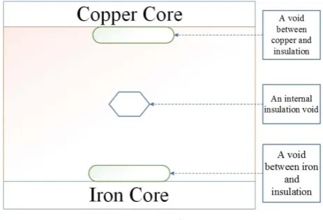
[image:1.595.315.547.359.517.2]Different PD types such as corona and surface discharges are observed from electrode edges, point edges or cylindrical wires in case of gases [11] [12]
[13]
. A schematic of PD activity in a high voltage system can be seen in the Figure 1.Figure 1. A schematic of PD activity.
Radio systems that are capable of localization have many applications [14]. Received signal strength (RSS) based localization can be range-based or range-free [15] [16]. Range based localization is strictly based on time synchronization and changes to the deployed systems are hard to implement due to synchronization. Techniques such as TOA, TDOA and DOA are all range based localization techniques [17]. Range free localization is purely based on the received signal strength and there are no synchronization requirements. For example, the work in [18] is based on localization of the source based on centroid point calculation. Similarly, the work in [19] utilizes the trilateration algorithm to estimate the location of the source.
Physical localization of the source is the key requirement of the proposed work. The main advantage of the source localization is that it can help to identify the source that requires decommissioning [20]. Keeping in view the simplicity and ease of implementation, the
proposed algorithm works purely based on the received signal strength and source coordinates are estimated by converting the received signal strength into distance. The RSS technique is based on Lateration or distance. The key advantage that RSSI based localizations offers over its counterparts such as AOA, TDOA or TOA is the scalability i.e. at any time an extra receiving node can be deployed that will improve the localization accuracy. This is a challenging task in TOA, TDOA or AOA based localizations due to time synchronization requirements.
A
PD pulse attenuates and distorts as it travels from the source to the measuring system. However, even distorted or attenuated PD pulses still contain significant information about the nature and the location of the discharge [21].II. ALGORITHM DESCRIPTION
The propagation of radio signals in free space will experience losses. Keeping in mind the loss, it is important to choose a propagation model that best suits the application. There are three types of propagation models that can be used for the given application. These include ground reflection, free space and shadowing model. In free space and ground reflection models, the received energy is a function of distance. This implies that signal transmission is isotropic i.e. coverage is an ideal circle [16].
Keeping in view that real PD signal is often anisotropic, the proposed algorithm is based on the path loss model equation as shown in equation (1):
= − 10
0 (1) is the measured signal strength by the receiving node, is the transmitted power of the source which is unknown, n is the path loss index (again it is unknown, however it can be constrained). and are the ℎ and reference node distances respectively.
The proposed algorithms can be summarized in the following steps
I. Assume an initial (universal) value of path loss index (n)
II. Use ratios of power received by a pair of sensors to calculate a locus for estimated PD location III. Repeat for all other pairs of sensors giving an
estimated location corresponding to each intersection of loci
IV. Calculate mean spatial location from all estimated locations
V. Calculate RMS spread of spatial location distance from mean location
VI. Repeat for multiple values of n and select the estimated mean location (as final estimated location) that has a minimum RMS spread
The location is estimated by converting the received signal into the distance. Equation (1) can be used to calculate the distance as given in equation (2):
= 10 (2)
The coordinates of the receivers that detect the signal emitted by the source are known and are named as (xi, yi),
the distance between the source, and the ℎ receiver can be calculated by using the equation below:
= ( − ) + ( − ) (3)
Equation (2) can be written in simplified form as below:
=
1010(4)
=
1010 (5)Taking the square of equation (2) and comparing equations (2) and (3) will give rise to the expression given in equation (6):
( − ) + ( − ) = (6)
In equation (6) corresponds to the distance of the reference node. Each node in the whole receiving system can be taken as the reference node, and the reference node offering the minimum error will be the one giving the optimum solution.
As the number of unknowns is two i.e. two coordinates of the unknown source, and the number of equations are more than two, a matrix equation is established and the solution of these equations is based on the linear least square approach.
The source transmitted power has been eliminated by using the ratio approach, however, the path loss exponent (PLE) is still unknown and makes it impossible to solve the matrix equations.
The PLE is still an issue and to overcome that an initial value of PLE is chosen. Normally the path loss exponent is constrained to be in the range of 1 ≤ ≤ 4 [22]. To overcome the issues, an initial value of PLE is chosen and mean spatial location is estimated from all estimated locations. The RMS spread is calculated as shown below
= 1 (7)
Where, is the location distance from the mean estimated location and is the RMS spread of the location distance.
III. RESULTS
The results were obtained by generating the PD in the free space environment. Ten different measurements were taken and eight measurement sensors nodes been used in total. PD signal was generated by using the PD emulator as shown in the Figure 2.
[image:3.595.306.542.233.468.2]The signal was generated by using an AC supply of 30kV and the PD emulator of Figure 2. Measurement sensors were placed over an 18 by 18 meters grid. Sensor nodes used for measurement consisted of four major sub-systems including the RF front end, signal conditioning, microcontroller and the wirelessHART unit. Such sensors are simple and cost-effective and can be deployed for continuous monitoring of PD [23]. A dipole receiving antenna has been used to receive the PD signal. The experimental study suggests that PD signal bandwidth remains between 50-800 MHz, the used passbands have a frequency range from 30 to 75 MHz and 255 to 320 MHz [23] [10]
Figure 2. PD emulator used to generate the PD signal.
The signal measurements were performed in free space. The spatial distance between the receiving nodes was kept the same and the position of the source was changed as shown in Table 1.
[image:3.595.57.290.307.482.2]
Table 1. True location of the source at ten positions Position
No. X (m) Y (m)
1 13.5 4.5 2 4.5 4.5
3 4.5 13.5
4 13.5 13.5
5 10 6 6 6 8 7 8 12 8 12 10 9 4.5 -4.5 10 13.5 0
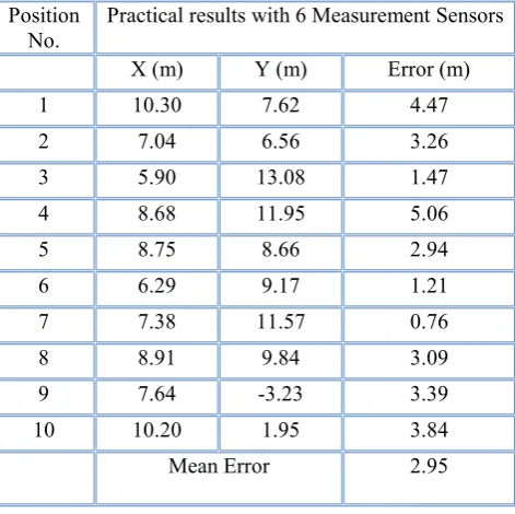
The location of the PD source was estimated by using six, seven and eight nodes respectively to see how an increase in the number of nodes affects the overall accuracy of the estimated location. Firstly, the location was estimated by using six nodes, and the estimated location of the source for all ten positions is shown in Table 2.
Table 2 shows the true versus estimated locations comparison with the error calculated for each location of the source. The mean error calculated is 2.95 meters. Results obtained for all ten positions were compared for true versus estimated location.
Table 2. Estimated location with 6 sensors
Position No.
Practical results with 6 Measurement Sensors
X (m) Y (m) Error (m)
1 10.30 7.62 4.47
2 7.04 6.56 3.26 3 5.90 13.08 1.47 4 8.68 11.95 5.06 5 8.75 8.66 2.94 6 6.29 9.17 1.21 7 7.38 11.57 0.76 8 8.91 9.84 3.09 9 7.64 -3.23 3.39
10 10.20 1.95 3.84
Mean Error 2.95
[image:3.595.316.522.512.682.2]An example result for position 1 is shown in Figure 3 where six measurement sensors were used.
Figure 3. Position 1 results with six measurement sensors.
[image:3.595.79.269.575.750.2]positions. Error calculations for individual positions suggest that accuracy has improved for majority of positions. Mean error calculated is 2.43 meters, which is 0.5 meters less than the error with six sensors. Same example result for position 1 with seven measurement sensors is shown in Figure 4.
Table 4 shows the results of the estimated locations when eight measurement sensors are used.
Table 3 Estimated location with 7 sensors
Position
No. Practical results with 7 Measurement Sensors X (m) Y (m) Error (m)
1 12.33 4.39 1.17
2 5.93 5.36 1.67 3 5.48 13.11 1.05 4 10.79 16.60 4.12
5 12.64 5.23 2.75
6 6.79 6.72 1.51 7 7.87 12.79 0.80 8 13.13 11.77 2.10 9 3.13 -6.13 2.12
10 14.38 -6.95 7.00
Mean Error 2.43
[image:4.595.279.534.89.524.2]
Figure 4. Position 1 results with seven measurement sensors.
It is clear from Table 4 that localization accuracy has improved when comparing to Tables 2 and 3. The mean estimated error is 2.19 meters which is lower than both Tables 2 and 3 results. The results for position 1 when eight measurement sensors are used are shown in Figure 5. The results obtained from all three scenarios show that estimation error is minimum when eight sensors are used. The localization accuracy gradually improves with an increase in the number of measurement sensors.
Table 4. Estimated location with 8 sensors
Position
No. Practical results with 8 Measurement Sensors X (m) Y (m) Error (m)
1 12.49 4.20 1.06
2 5.72 5.45 1.55
3 4.08 14.19 0.81
4 11.33 14.51 2.40
5 12.54 4.90 2.76
6 5.61 10.47 2.51
7 8.85 12.87 1.21
8 13.20 11.99 2.33
9 3.92 -5.58 1.22
10 14.23 -6.05 6.09
Mean Error 2.19
Figure 5. Position 1 results with eight measurement sensors.
IV. CONCLUSION
A novel PD localization algorithm has been proposed and location estimation has been performed in a real PD environment. There were ten different positions and for each position location estimation was performed by using six, seven and eight sensors respectively. It was concluded that as the number of sensors increases, the localization accuracy improves. Eight sensors seem to be enough for a good working accuracy.
ACKNOWLEDGMENT
The authors acknowledge the Engineering and Physical Sciences Research Council for their support of this work under grant EP/J015873/1.
V. REFERENCES
[image:4.595.57.283.204.611.2]regression approach," IET science, measurement & technology, vol. 12, no. 2, pp. 230-236, 2018. [2] H. Illias, S. T. Yuan, A. H. Abu Bakar, H. Mokhlis,
G. Chen and P. L. Lewin, "Partial discharge patterns in high voltage insulation," in IEEE International conference on Power and Energy (PECon), Kota Kinabalu, Malaysia, 2012.
[3] Y. Zhang, D. Upton, A. Jaber, H. Ahmed, B. Saeed, P. Lazaridis, P. Mather, A. Mopty, C. Tachtatzis, M. Judd and I. Glover, "Radiometric Wireless Sensor Network Monitoring of Partial Discharge Sources in Electrical Substations," International Journal of Distributed Sensor Networks, vol. 11, no. 9, pp. 1-9, January 2015.
[4] A. M. Gataullin, "Recording and processing of partial discharge signals," Instruments and Experimental Techniques, vol. 57, no. 4, pp. 426-430, 2014.
[5] H. Mohamed, P. Lazaridis, D. Upton, U. Khan, B. Saeed, A. Jaber, I. Glover and M. Viera, "Partial Discharge Detection Using Low Cost RTL-SDR Model for Wideband Spectrum Sensing," in
International Conference on Telecommunication, Thessaloniki, Greece, 2016.
[6] P. Miao, X. Li, H. Hou, G. Sheng, Y. Hu and X. Jiang, "Location algorithm for partial discharge based on radio frequency (RF) antenna array," in
Power and Energy Engineering Conference (APPEEC), 2012 Asia-Pacific, Shanghai, China, 2012.
[7] P. J. Moore, I. E. Portugues and I. A. Glover , "Radiometric location of partial discharge sources on energized high-Voltage plant," Power Delivery, IEEE Transactions, vol. 20, no. 3, pp. 1-9, 2005. [8] H. Mohammed, P. Lazaridis, D. Upton, U. Khan, K.
Mistry, P. Mather , M. Vieira, K. Barlee, D. Atkinson and I. Glover, "Partial Discharge Localization Based on Received Signal Strength," in
23rd International Conference on Automation and Computing (ICAC), Huddersfield, UK, 2017. [9] H. Mohamed, P. I. Lazaridis, U. Khan, B. Saeed, K.
Mistry, D. Upton, P. J. Mather and I. A. Glover, "Partial Discharge detection in smart grid using Software Defined Radio," in TELFOR 2017, Belgrade, Serbia, 2017.
[10] A. A. Jaber, P. I. Lazaridis, M. Moradzadeh, I. A. Glover, Z. D. Zaharis, M. F. Vieira, M. D. Judd and R. C. Atkinson, "Calibration of Free-Space Radiometric Partial Discharge Measurements,"
IEEE Transactions on Dielectrics and Electrical Insulation, vol. 24, no. 5, pp. 3004 - 3014, 2017. [11] H. Xiong, C. Zhiyuan , W. An and B. Yang, "Robust
TDOA Localization Algorithm for Asynchronous Wireless Sensor Networks," International Journal of Distributed Sensor Networks, pp. 1-10, 2014. [12] M. D. Judd, "Radiometric partial discharge
detection," in International Conference on
Condition Monitoring and Diagnosis, Beijing, China, 2008.
[13] H. Mohamed, P. Lazaridis, D. Upton, U. Khan, A. Jaber, B. Saeed, P. Mather and I. Glover, "Partial discharge detection using software defined radio," in
International Conference for Students on Applied Engineering (ICSAE), Newcastle upon Tyne, UK, 2016.
[14] A. Seyed and M. Buehrer, Handbook of position location: Theory, practice and advances, John Wiley and sons , 2012.
[15] A. A. Momtaz , F. Behnia , R. Amiri and F. Marvasti, "NLOS Identification in Range-Based Source Localization: Statistical Approach," IEEE Sensors Journal, vol. 18, no. 9, pp. 3745 - 3751, 28 February 2018.
[16] H. Shi, "A New Weighted Centroid Localization Algorithm based on RSSI," in International Conference on Information and Automation, Shenyang, 2012.
[17] J. M. Fresno , G. Robles, J. M. Martínez-Tarifa and B. G. Stewart, "Survey on the Performance of Source Localization Algorithms," Sensors, vol. 17, no. 11, pp. 2-25, 2017.
[18] Y.-C. Cheng, Y. Chawathe, A. LaMarca and J. Krumm, "Accuracy characterization for metropolitan-scale Wi-Fi localization," in MobiSys '05Proceedings of the 3rd international conference on Mobile systems, applications, and services, 233-245, 2005.
[19] A. Savvides, C.-C. Han and M. B. Strivastava, "Dynamic fine-grained localization in Ad-Hoc networks of sensors," in MobiCom '01 Proceedings of the 7th annual international conference on Mobile computing and networking, Rome, Italy, 2001. [20] G. Robles, J. M. Fresno, M. Sánchez-Fernández and
J. M. Martínez-Tarifa, "Antenna Deployment for the Localization of Partial Discharges in Open-Air Substations," Sensors, vol. 16, no. 4, 2016.
[21] Z. D. Wang, P. A. Crossley, k. J. Cornick and D. H. Zhu, "An algorithm for partial discharge location in distributed power transformers," in IEEE Power Engineering Society, 2000.
[22] N. Patwari, J. N. Ash, S. Kyperountas, A. O. Hero, R. L. Moses and N. S. Correal, "Locating the nodes: cooperative localization in wireless sensor networks," IEEE Signal Processing Magazine, vol. 22, no. 4, pp. 54 - 69, 27 June 2005.