MODEL PREDICTIVE CONTROL APPLICATION
TO SPACECRAFT RENDEZVOUS IN MARS
SAMPLE RETURN SCENARIO
M. Saponara
1, V. Barrena
2, A. Bemporad
3, E. N. Hartley
4,
J. Maciejowski
4, A. Richards
5, A. Tramutola
1,
and P. Trodden
5 1Thales Alenia Space (TAS) Italia253 Strada Antica di Collegno, Torino 10146, Italy
2GMV
11 Isaac Newton, PTM Tres Cantos, Madrid 28760, Spain
3Department of Mechanical and Structural Engineering University of Trento
Trento, Italy
4Department of Engineering, University of Cambridge
Cambridge, U.K.
5Department of Aerospace Engineering, University of Bristol
Bristol, U.K.
Model Predictive Control (MPC) is an optimization-based control strat-egy that is considered extremely attractive in the autonomous space rendezvous scenarios. The Online Recon¦guration Control System and Avionics Architecture (ORCSAT) study addresses its applicability in Mars Sample Return (MSR) mission, including the implementation of the developed solution in a space representative avionic architecture system. With respect to a classical control solution High-integrity Au-tonomous RendezVous and Docking control system (HARVD), MPC al-lows a signi¦cant performance improvement both in trajectory and in propellant save. Furthermore, thanks to the online optimization, it al-lows to identify improvements in other areas (i. e., at mission de¦nition level) that could not be knowna priori.
1
INTRODUCTION
Within AURORA programme, the MSR mission is the main planned objective in the international e¨ort on the Solar System exploration. Its main goal is to bring back to the Earth a sample of Martian soil. A number of new technologies will be
© Owned by the authors, published by EDP Sciences, 2013
required to carry out this pioneering mission and one of them is the rendezvous and capture system, which will be able to detect, approach, and capture the sample of Martian soil, previously put in a prede¦ned orbit by the Mars Ascent Vehicle (MAV).
Although autonomous docking is now a well established technology, au-tonomous capture (with a poorly cooperative target) is more delicate. The de-velopment of a Guidance, Navigation and Control system (GNC) for rendezvous and capture has been addressed in the European Space Agency (ESA) study named HARVD. This study has been separated into two parallel activities, one of them lead by GMV in collaboration with TAS France and Italia. The devel-oped solution shows that, with classical control techniques, it is possible to have an automated rendezvous and capture control system with preplanned operations able to ful¦ll the MSR capture requirements.
Starting from HARVD experience, a further study has been de¦ned, named ORCSAT. The objective of the study is to improve the HARVD GNC by means of optimization-based control strategies such as MPC. The work on this study was supported by the ESA under contract No. 22421.
Model predictive control (see, for example, [1 3]) is an advanced control technique which uses a prediction model and numerical optimization methods to obtain a sequence of control inputs that minimizes a function of the control inputs and predicted plant state trajectory over a given time horizon, subject to constraints. At each sampling instant, the optimization performed based on new measurement data, and the ¦rst control input of the sequence is applied. The remainder of the sequence is discarded and the process is repeated at the next sampling instant in a ¤receding horizon¥ manner. Whilst MPC has its origins in the chemical process industries [4], there is increasing interest in its application to vehicle manoeuvre problems [5 7], including spacecraft trajectory control [8 11] and attitude control [12 14]. Essentially, the application of MPC builds upon the ideas of fuel and time-optimal trajectory planning by bringing the optimization onboard, providing a natural framework for increased autonomy and recon¦gurability, whilst accounting for physical and operational constraints such as ¦nite control authority, passive safety, and collision avoidance.
The ORCSAT study considers also the developing of an MPC Framework software (SW) tool (MPCTOOL) for supporting the design, analysis and sim-ulation of MPC-based control systems as well as the development of embedded model predictive controller for autonomous rendezvous control systems. Fur-thermore, another key point of the ORCSAT study is the implementation of the developed MPC control system into a space representative avionic architecture system.
2
THE HIGH-INTEGRITY AUTONOMOUS
RENDEZVOUS AND DOCKING CONTROL
SYSTEM STUDY
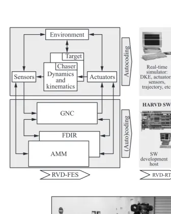
In the last years, the number of studies considering rendezvous and docking/ capture missions around Mars or other planets/asteroids has signi¦cantly in-creased. As a consequence, it is surely worth dedicating e¨ort to consolidate maturity of GNC technologies for such missions, in order to have onboard sys-tems with a higher and higher level of autonomy, robustness, and safety, with the ¦nal objective of decreasing costs and increasing the probability of mission success. Following this tendency, a team led by GMV and including, among others, TAS, has developed HARVD, an ESA-funded activity implementing a GNC / Autonomous Mission Management (AMM) / Fault Detection, Isolation, and Recovery onboard SW for rendezvous and docking/capture scenarios around Mars, Earth, or potentially other planets [15 17]. The HARVD, based on radio frequency (RF), camera, and LIDAR (light detecting and ranging) measure-ments, includes design, prototyping, and veri¦cation at three di¨erent levels: algorithms design and veri¦cation in a High-Fidelity Functional Engineering Simulator, SW demonstrator to be veri¦ed in Real Time (RT) Avionics Test Benching and Dynamic Test Benching. Rendezvous and capture on an elliptic orbit have been specially addressed, demonstrating the technical feasibility and the potential propellant saving.
The HARVD stepwise development and veri¦cation approach is shown in Fig. 1.
The Development, Veri¦cation, and Validation (DVV) approach in the HARVD activity relies on the use of COTS SW tools:
Matlab/Simulink/State§ow from Mathworks, including associated tool-boxes, for design, analysis, simulation, and validation of system models and algorithms;
TargetLink from dSPACE for automatic generation of production code (C code) straight from the above graphical development environment; and
dSPACE simulator for RT development/simulation environment.
the results obtained are very encouraging for the consolidation of higher Tech-nology Readiness Levels. Mars ascent vehicle circularization failures have been also taken into account, resulting in a number of elliptic target orbit rendezvous scenarios for which HARVD has demonstrated to be fully ready.
The development of RT test bench has been concluded and the acceptance RT test campaign has been successfully completed. The RT test bench is based on a LEON board GR-PCI-XC2V @45 MHz, and computational load margins of 32% have been achieved for the Worst Case Execution Time (WCET).
Recently, the tailoring of the GMV Dynamic Test Bench (PLATFORM, see Fig. 1) has already started, and the dynamic tests are foreseen to be executed in the next few months.
3
THE MPCTOOL
MPCTOOL is a MATLAB/Simulink toolbox providing all major features for the design, analysis, and simulation of model predictive controllers based on linear time-invariant (LTI) or linear time-varying (LTV) models, as well as for auto-matic code-generation of embedded model predictive controllers. MPCTOOL is tailored (although not limited) to the synthesis of autonomous rendezvous con-trol systems. The inclusion of LTV capability is a key enabler for rendezvous, since elliptical orbits and J2 e¨ects introduce time variation into the dynamics. MPCTOOL extends the Model Predictive Control Toolbox from The Math-works, Inc. [18] to introduce new features, modifying existing MATLAB objects, adding new functions (MATLAB methods) based on them, introducing new ob-jects and their methods, extending the C code of the S-Function behind the basic LTI-MPC controller, and introducing new Simulink blocks coded in Em-bedded MATLAB (EML) for LTV-MPC. Model predictive controllers designed for LTI systems can be converted to explicit form [19] via the direct link be-tween MPCTOOL and the Hybrid Toolbox for MATLAB [20]. Furthermore, a new Dual-Simplex solver has been developed to manage optimization prob-lems expressed as a Linear Programming (LP) problem [21]. The new features introduced by MPCTOOL on top of the existing MPC Toolbox are the following:
the ability to set terminal weights and constraints in LTI-MPC (including in¦nite-horizon MPC);
handle variable-horizon MPC problems in which the horizon length is op-timized online;
handle quantized inputs in LTI-MPC problems;
return the optimal cost of MPC for comparing and choosing the best action among a set of model predictive controllers;
allow the speci¦cation of convex piecewise a©ne stage costs (such as abso-lute values) on inputs and outputs;
handle arbitrary linear constraints on combinations of inputs and outputs; and
handle arbitrary linear time-varying models, weights, constraints, and hori-zons by providing two Simulink blocks based on EML code, supporting both quadratic programming (QP) and LP problem formulations.
The latter feature, namely, LTV-MPC based on LP, was employed in the studies described in this paper and will be detailed next.
The LTV model predictive controller relies on the following rather general linear time-varying prediction model:
x(j+Ts) =A(j, x(t))x(j) +B(j, x(t))u(j) +f(j, x(t)) ;
y(j) =C(j, x(t))x(j) +D(j, x(t))u(j) +g(j, x(t)) ;
z(j) =Ez(j, x(t))(y(j)−r(j)) +Hz(j, x(t))(u(j)−ur(j))
+Pz(j, x(t))–u(j) ;
c(j) =Ec(j, x(t))x(j) +Hc(j, x(t))u(j) +Pc(j, x(t))–u(j) ⎫ ⎪ ⎪ ⎪ ⎪ ⎪ ⎪ ⎪ ⎪ ⎪ ⎪ ⎬ ⎪ ⎪ ⎪ ⎪ ⎪ ⎪ ⎪ ⎪ ⎪ ⎪ ⎭ (1)
where Ts is the sampling time; k is the prediction step; t is the current time,
j=t+kTs is the prediction time;xis the state vector;uis the input vector;y is the output vector; –u(j) = u(j)−u(j−Ts) is the input increment; ris the output reference vector;uris the input reference;zis the ¤performance vector¥ to be optimized; c is the ¤constrained vector;¥ and A, B, f, C, D, g, E, H, andP are (possibly time-varying and state-dependent) matrices.
The MPC optimal problem to be optimized at each timetis
min ρ11+ρ22+
N(4t)−1
k=0
z(j)1;
s.t. –umin(j)≤–u(j), k= 0, . . . , N(t)−1 ;
c(j)≤cmax(j) +Vcρ1, k= 0, . . . , N(t)−1 ;
CN(t)x(t+N(t)Ts)≤dN(t) +VNρ2
⎫ ⎪ ⎪ ⎪ ⎪ ⎪ ⎪ ⎪ ⎪ ⎬ ⎪ ⎪ ⎪ ⎪ ⎪ ⎪ ⎪ ⎪ ⎭ (2)
where N(t) ≤ Nmax is the prediction horizon; and ρ1 and ρ2 are the slack
The optimal control problem (2) is mapped into the LP
min ρ11+ρ22+
N(4t)−1
k=0
l 4 i=1
di(j) ;
s.t. di(j)≥ ±zi(j), di(j)≥0,
+ MPC constraints
⎫ ⎪ ⎪ ⎪ ⎪ ⎬ ⎪ ⎪ ⎪ ⎪ ⎭
(3)
which has (m+l)N(t) + 1 optimization variables and, besides the nonnegativity constraints –u−–umin≥0,≥0,di(j)≥0, 2lN(t) constraints to express the
1-norm in (3), plus as many constraints as the ones that are optionally de¦ned in (2).
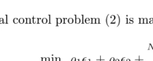
[image:7.612.163.319.141.203.2]The user can exploit the maximum §exibility o¨ered by the EML language to de¦ne the prediction model (1) and all the parameters appearing in the MPC op-timization problem (2) in an EML module, which is then used by the LTV-MPC Simulink block to construct and solve problem (3). Accordingly, as depicted in Fig. 2, the block contains an LP builder function and a Dual Simplex LP solver coded in EML code, implementing the LTV-MPC formulation described above. The block is §exible enough to allow an arbitrary number of parameters enter-ing the EML prediction model from the Simulink diagram as RT varyenter-ing signals, to vary online prediction and control horizons, to limita priori the maximum number of LP iterations.
4
THE ORCSAT MPC DESIGN
4.1 Control System Architecture and Choice of Prediction Model
Fi
gure
2
Si
m
ul
ink
di
a
g
ra
m
unde
rl
yi
ng
the
L
P
-ba
se
d
L
T
V
-M
P
C
bl
o
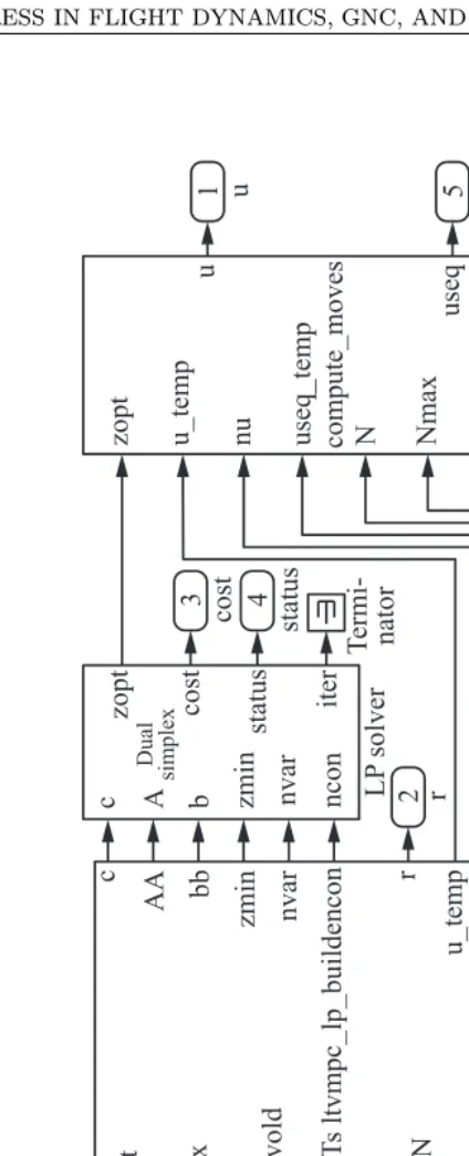
[image:8.612.122.334.113.635.2]Table 1 Rendezvous phases
Phase Requirement
Orbit Synchronization Transla-tional Guidance (OSTG)
To bring chaser from a distance of approx-imately 300 km into the same orbit as the target, with an in-track separation of be-tween 5 and 30 km on either side of the target
Impulsive Nominal Translational Guidance (INTG)
To perform passively safe impulsive trans-fers between a sequence of prede¦ned hold-ing points in the same orbit as the tar-get until an in-track separation of 100 m is reached
Forced Terminal Translational Guidance (FTTG)
To track a straight-line trajectory from 100- to 3-meter separation from the target such that a subsequent free-drift trajectory captures the target with a 20-centimeter tolerance
Collision Avoidance Manoeuvre (CAM)
To bring the chaser to a safe distance, fur-ther than 5 km from the target within 3 or-bits, avoiding collision in the process
is passive, νtgt can be calculated as a function of time using Kepler£s
equa-tion [30], thus allowing a linear time-varying representaequa-tion of the relative dy-namics.
The objective of the MPC control system designed during this study is to bring the chaser craft from the point of target detection at a range of approxi-mately 300 km, via a sequence of holding points in the same orbit as the target, to a ¤blinding point¥ approximately 3 m from the target, at which point it should be moving towards the target at an in-track velocity of 0.1 m/s. Target capture is then completed on a passive drift trajectory. The MPC system pro-vides both guidance and control and is not restricted to tracking predetermined trajectories.
4.1.1 Orbit synchronization translational guidance
The ¦rst phase, Orbit Synchronization Translational Guidance (OSTG), has the objective of bringing the chaser from a distance of approximately 300 km into the same orbit as the target using thrusters, with an in-track separation of be-tween 5 and 30 km on either side of the target, whilst minimizing propellant consumption and manoeuvre time. At these ranges, short-term control accuracy is not critical; so, a relatively long prediction time can be used. However, long-term prediction accuracy is important in order to perform optimal manoeuvres. For these reasons, the J2-modi¦ed Gauss£s variational equation (GVE)
predic-tion model of [9] is chosen. This predicts the relative trajectory between the chaser and target in terms of the relative Keplerian orbital elements rather than relative positions and velocities in a rectangular or cylindrical coordinate frame, whilst using the Gim Alfriend [29] approach of incorporating the e¨ects ofJ2to
account for variations in gravity due to the oblateness of the central body of the orbit. Because the relative orbital elements are small, despite large Euclidean separations, the e¨ects of linearisation error are small in comparison to predic-tion models such as those of [22,28], which use rectangular or cylindrical relative coordinates. The system input is assumed to be an impulsive change in velocity (–V) in a local orbital reference frame centered on the chaser.
4.1.2 Impulsive nominal translational guidance
The second phase, Impulsive Nominal Translational Guidance (INTG), must per-form a sequence of passively safe impulsive transfers between a sequence of pre-de¦ned holding points until an in-track separation of 100 m is reached. Greater control accuracy is required during this phase, necessitating a shorter sampling period. In addition, collision avoidance constraints must be more ¦ne-grained. However, as the OSTG phase will have reduced much of the radial and out-of-plane separation between chaser and target, the e¨ect of linearization error on the Yamanaka Ankersen [28] equations is no longer a problem, as long as a cylindrical relative coordinate system is used [26]. This model is less complex than theJ2-modi¦ed GVEs and allows objectives and constraints to be directly
speci¦ed in the cylindrical frame without requiring a linearized geometric trans-formation (with inevitable loss of accuracy) from the relative orbital elements. The prediction model input is assumed to be an impulsive –V in the cylindrical target orbital frame.
4.1.3 Forced terminal translational guidance
to a position 3 m from the target from where it can capture the target on a free drift trajectory. Radial, in-track, and out-of-plane separation are small during this phase. Control accuracy is critical due to the tight capture tolerances, and a much higher sampling rate is required than for other phases. As for the INTG phase, the Yamanaka Ankersen [28] equations are used for the trajectory prediction model.
In addition, to maintain target pointing, the model predictive controller must also handle attitude regulation to an externally provided setpoint, using thrusters. A linearized quaternion-based prediction model [13] extended to con-sider the elliptical orbital dynamics is used for the relative attitude control. The attitude reference frame used for control is chosen depending on the direc-tion of approach, and the attitude setpoint in the inertial frame to avoid the predicted trajectory crossing the discontinuity at±180◦in the quaternion repre-sentation [33]. Because the prediction matrices are rebuilt at each time step due to the LTV prediction model, the opportunity is taken to relinearize the attitude dynamics about the current measured attitude at each time step.
4.1.4 Collision avoidance manoeuvre
The CAM must safely move the chaser away from the target, to a distance of 500 m within three orbits without collision with the target. Essentially, this objective is similar to that of INTG, except traveling away from the target instead of towards it, and with a less speci¦c terminal objective. It, therefore, makes sense to use the Yamanaka Ankersen prediction model for this phase also.
4.2 Model Predictive Control Subsystem Design
Each of the model predictive controllers is designed independently, but with a common interface and a common output function to convert the –V into ¦nite-duration thrust pulses in the inertial frame. The core MPC function of each control subsystem is implemented using the blocks from the MPCTOOL, with the linear time-varying prediction models implemented as EML functions called by the MPCTOOL blocks. Any additional logic or reference-frame changes are implemented using Simulink blocks.
4.2.1 Orbit sinchronization translational guidance model predictive controller
Figure 3 The OSTG safety (a) and terminal (b) constraints
encode the minimization of total propellant consumption, the model predictive controller must minimize the absolute sum of –V applied over the prediction horizon [34]. Furthermore, to balance this with time to completion, a termi-nal constraint enforcing the completion criteria is imposed at the end of the prediction horizon, and the prediction horizon itself is included as a decision variable in the cost function [6, 35, 36]. Letting N be the prediction horizon,
u= [u(t+Ts|t)T,· · ·, u(t+ (N−1)Ts|t)T]T andαbe a parameter determining
constraints that will be described later, the cost function is:
JOSTG(α,u, N) =N+
N#−1
k=1
wuu(t+kTs|t)1 .
Note that the summation is from k = 1 not k = 0, implying that the input calculated at the current time step is applied at the next time step to allow su©cient time duration for computation to occur. The terminal constraint, which will be described later, ensures that the predicted trajectory ends in the correct orbit, with an acceptable separation from the target.
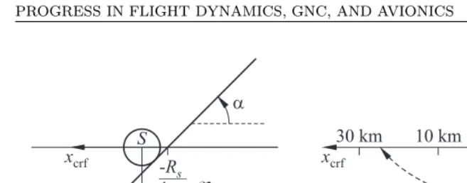
In order the predicted trajectories do not collide with the target, constraints are placed on the predicted trajectories to ensure that they do not enter a safety sphere of radiusRs(t), surrounding the target. In addition, as proposed in [10], unforced drift trajectories emanating from each point in the prediction horizon are also constrained to ensure passive safety. Collision avoidance is a manifestly nonconvex constraint, but it is approximated by a half-space constraint with angle relative to the in-track direction parameterized by α(Fig. 3). The value ofαthen determines on which side of the target the terminal constraint places the end of the predicted trajectory.
the current angle between the chaser and the zcrf axis, rounded to the nearest
45◦, by solving 3N convex optimizations, varying N between 1 and Nmax, for
each α ∈ {α0 −45◦, α0, α0 + 45◦} using two nested Simulink ¤For-iterator¥
subsystems, the control sequence can be found that minimizes the overall cost function. A sampling period TS = 600 s was chosen, along with a maximum prediction horizonNmax= 25.
4.2.2 Impulsive nominal translational guidance model predictive controller
The INTG model predictive controller must transfer the chaser between a se-quence of invariant holding points onV (i. e., the in-track axis in the cylindrical orbital frame) until a separation of 100 m is achieved. Because release from these holding points must be governed by an external signal, there is no point predict-ing further ahead than the end of a spredict-ingle transfer. It is su©cient to design a controller to perform a transfer, parameterized by the distance from the target of the next holding point.
The design is similar to that of the OSTG model predictive controller in that a 1-norm cost function is used in conjunction with a variable horizon im-plemented by solving multiple convex optimizations. However, the cost function includes distance instead of time to re§ect that fuel consumption is proportional to distance traveled rather than time when carrying out passively safe hopping trajectories. The holding points are scheduled by an external algorithm and parameterized by distancexhp. The cost function is
JINTG(u, N) =
N#−1
k=1
Ec(xcrf(t+kTs|t)−r(t+kTs))1+wuu(t+kTs|t)1
wherer(t+kTs) = [±xhp(1 +etgtcosνtgt(t+kTs)), 0, 0, 0, 0, 0] T
depends on the direction of approach; xcrf is the state vector in the cylindrical reference
frame;etgt is the eccentricity of the target orbit;νtgt is the true anomaly of the
target; and
Ec=
1 0 0 0 0 0 0 1 0 0 0 0
.
As for the OSTG model predictive controller, passive safety constraints are imposed over a period of one orbit from each prediction in the control horizon. In addition, to ensure passive safety over a longer period, an additional passive drift constraint is imposed to make sure that long-term secular drift is away from the target (thus avoiding collision in subsequent orbits). LettingAorb(νtgt) be
the propagation matrix for a whole orbit,
The terminal set for the INTG model predicted controller is de¦ned as a box with side-length 2(etgt+0.1), centered on a pointxhpaway from the target onV,
with an additional constraint that the chaser should be on a periodic trajectory and also be inside the box after1/
4,1/2, and3/4orbits of free drift. A sampling
periodTs= 300 s and a maximum prediction horizon ofNmax= 20 were chosen.
4.2.3 Forced terminal translational guidance model predictive controller
During the FTTG phase, trajectory and attitude tracking accuracy becomes more important than long-term fuel minimization. The navigation uncertainty is of a similar order of magnitude to the expected tracking errors; so, a conventional quadratic cost function is appropriate. The controller is implemented using the ¤QP-based LTV model predictive controller¥ block from MPCTOOL, with a sampling periodTs = 3 s and a prediction horizonN = 15. Letting x(j|t) be the combined position, velocity, attitude quaternion, and angular velocity states,
r(j) the corresponding reference setpoint, andu(j|t) the vector of thruster inputs, the cost function is:
JFTTG=
N#−1
k=1
(x(t+kTs|t)−r(t+kTs))TQ(x(t+kTs|t)−r(t+kTs))
+ –u(t+kTs|t)TR–u(t+kTs|t).
Changes in input (–u) are penalized instead of the absolute input value to enable o¨setfree tracking of forced-equilibrium setpoints [37]. Positivity and saturation constraints are applied to inputs. The reference trajectoryr(j) and cost function weightings Q ≥ 0 and R ≥ 0 are chosen so that the controller tracks an attitude setpoint, a position in the radial and out-of-plane directions, and an approach velocity in the in-track direction.
4.2.4 Collision avoidance manoeuvre model predictive controller
chosen so that under the speci¦ed worst-case navigation error, the chaser will be further than 500 m away from the target in three orbits. The INTG model predictive controller can then hold the chaser in a periodic §y-around orbit or restart approach via its sequence of holding points once the CAM is complete.
5
THE ONLINE RECONFIGURATION CONTROL
SYSTEM AND AVIONICS ARCHITECTURE
The avionic architecture considered in HARVD is based on the ¤Aurora Avionics Architecture¥ ESA study, which is the avionics reference for future exploration vehicles. From this starting point, the ORCSAT study includes the design of an Avionic Architecture System allowing the implementation of embedded MPC-based systems. The MPC concept is MPC-based on the optimization of a cost function under some constraints, which usually is carried out using quite complex iter-ative algorithms, requiring high computational capability. Therefore, the main challenge of the avionic architecture design is to de¦ne a Central Data Man-agement Unit (CDMU) able to cope with the MPC needs. In particular, the selection of the Central Processing Unit (CPU) is the key for the MPC embed-ded implementation.
Since the beginning of the design, it was evident that a CPU composed of a processor and a coprocessor has to be considered as baseline (distributed archi-tecture) taking into account available space quali¦ed processor computational performances (Fig. 4). This solution allows a distribution of the complete on-board SW on the two processors leaving to the coprocessor the execution of GNC algorithms requiring signi¦cant computational throughput (MPC) and to the processor the handling of the system units, the other parts of the GNC, etc. The next step was the selection of the processors. Currently space-quali¦ed processors are based on LEON2 FT, with performance of 86 MIPS, 23 MFLOPS at 100 MHz: taking into account also the HARVD experience, it has been con-sidered adequate for the central processor of the CDMU.
Regarding the coprocessor, the MPC computational throughput is the driver for the selection. To support this task, pro¦ling of the MPC algorithm was performed using Simulink features, to evaluate the time needed for the execution of the MPC algorithms. Afterwards, these timing values have been scaled to the selected processor exploiting the Whetstone benchmark. The processors selected for the trade-o¨ are the LEON2 FT and PowerPC750FX, able to perform 1650MIPS at 733 MHz which has been used to design space-quali¦ed boards like the Maxwell SCS750.
con-Fi
gure
4
Cen
tral
d
at
a
m
an
agemen
t
u
n
it
w
it
h
d
ist
rib
u
ted
arc
h
it
ect
u
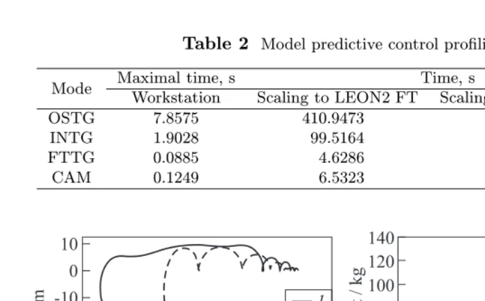
[image:16.612.77.391.132.622.2]Table 2 Model predictive control pro¦ling
Mode Maximal time, s Time, s
Workstation Scaling to LEON2 FT Scaling to PowerPC 750FX
OSTG 7.8575 410.9473 23.7401
INTG 1.9028 99.5164 5.7490
FTTG 0.0885 4.6286 0.2674
[image:17.612.67.406.144.211.2]CAM 0.1249 6.5323 0.3774
Figure 5 The HARVD (1) vs. MPC (2) performance comparisons
trol step of 3 s. Instead, the PowerPC 750FX shows timings which are widely compatible with the MPC design and expected computational capabilities and, therefore, it has been selected as baseline for the CPU coprocessor.
6
SIMULATION RESULTS AND COMPARISONS
Figure 5 shows the comparison between the simulation results obtained with the HARVD GNC solution and the ones obtained with the MPC in the case of rendezvous circular orbit. Di¨erences are visible since the beginning of the rendezvous, where the MPC trajectory remains closer to the target with respect to HARVD, but the most signi¦cant result is the propellant save, which in this case is about 35 kg.
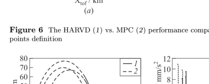
there-Figure 6 The HARVD (1) vs. MPC (2) performance comparisons with new holding points de¦nition
Figure 7 The CAM simulation results: 1 ¡ §y-around and2¡ CAM
fore, the HARVD simulation has been repeated with the ¦rst holding point at 20 km. Figure 6 shows that HARVD performance improved a lot, in particular, on the propellant consumption: in this case, the di¨erence is reduced to about 10 kg.
This aspect is quite important: the online optimization performed by MPC has permitted the detection of a possible improvement in the nominal mission scenario (i. e., de¦nition of the holding points) that would be di©cult to clearly identifya priori.
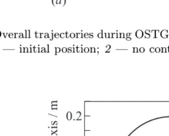
[image:18.612.67.405.300.437.2]Figure 8 Overall trajectories during OSTG and INTG of 50 cases of the Monte-Carlo campaign: 1 ¡ initial position;2 ¡ no control;3 ¡ OSTG; and4 ¡ INTG.
Figure 9 Capture performance of 400 test cases of the Monte-Carlo campaign: 1¡ 20-centimeter requirement; and2¡ target center
The MPC solution has been also validated and veri¦ed by means of a Monte-Carlo simulation campaign composed by 800 test cases, in order to test the performance of the control in di¨erent scenarios (circular and elliptic orbit) and starting from di¨erent initial relative positions and dynamics with respect to the target. The obtained results are very good, since the capture has been always achieved with margins.
[image:19.612.150.317.319.454.2]7
CONCLUDING REMARKS
Optimization-based control techniques like MPC are considered extremely at-tractive for applications which require high level of autonomy, optimal path planning, and dynamic safety margins. The ORCSAT study is addressing the usage of the MPC techniques on the rendezvous and capture scenarios of the MSR mission. The results obtained after the design phase are encouraging, since with respect to classical control techniques (HARVD), it is possible to have a signi¦cant improvement, in particular, in the propellant consumption. As side e¨ect, but not less important, online optimization could drive the de¦nition of higher level mission aspects that could not be easy to address in the earlier phase of GNC design.
The MPC design has been veri¦ed and validated throughout a wide Monte-Carlo simulation campaign which considers plant mismatch, sensors and actua-tors failures, and di¨erent initial dynamic conditions. Obtained results con¦rm the robustness of the design and the very good performance.
The next step of the ORCSAT study will be the implementation of the MPC algorithms in the selected avionic architecture, with the objective to test the RT performance of the developed solution on a §ight-representative avionic. In the end, the GMV Dynamic Test Bench will be enhanced with the model predictive based control and the selected avionics for the ¦nal dynamic test campaign.
REFERENCES
1. Maciejowski, J. M. 2002.Predictive control with constraints. Pearson Education. 2. Camacho, E. F., and C. Bordons. 2004.Model predictive control. London:
Springer-Verlag.
3. Rawlings, J. B., and D. Q. Mayne. 2009. Model predictive control: Theory and design. Nob Hill Publishing.
4. Qin, S. J., and T. A. Badgwell. 2003. A survey of industrial model predictive control technology.Control Eng. Practice11(7):733 64.
5. Shim, D. H., H. J. Kim, and S. Sastry. 2003. Decentralized nonlinear model pre-dictive control of multiple §ying robots. 42nd IEEE Conference on Decision and Control Proceedings. 4:3621 26. Maui, Hawaii, USA.
6. Richards, A., and J. P. How. 2006. Robust variable horizon model predictive control for vehicle maneuvering.Int. J. Robust Nonlinear Control16(7):333 51.
7. Almeida, F. A. 2008. Waypoint navigation using constrained in¦nite horizon model predictive control. AIAA Guidance, Navigation and Control Conference and Ex-hibit Proceedings. Honolulu, Hawaii.
9. Breger, L., and J. P. How. 2007. Gauss£s variational equation-based dynamics and control for formation §ying spacecraft.J. Guidance Control Dyn.30(2):437 48. 10. Breger, L., and J. P. How. 2008. Safe trajectories for autonomous rendezvous of
spacecraft.J. Guidance Control Dyn.31(5):1478 89.
11. Bodin, P., R. Noteborn, R. Larsson, and C. Chasset. 2011. System test results from the GNC experiments on the PRISMA in-orbit test bed.Acta Astronautica
68(7-8):862 72.
12. Manikonda, V., P. O. Arambel, M. Gopinathan, R. K. Mehra, and F. Y. Hadaegh. 1999. A model predictive control-based approach for spacecraft formation keeping and attitude control.American Control Conference Proceedings. San Diego, CA. 6:4258 62.
13. Hegrenˆs, O., J. T. Gravdahl, and P. Tondel. 2005. Spacecraft attitude control using explicit model predictive control.Automatica41(12):2107 14.
14. Wood, M., and W. H. Chen. 2008. Model predictive control of low Earth orbiting satellites using magnetic actuation. Proc. of the Institution of Mechanical Engi-neers, Part I: J. Syst. Control Eng. 222(6):619 31.
15. Colmenarejo, P., L. Tarabini, C. Le Peuv‚edic, and A. Guiotto. 2008. HARVD devel-opment, veri¦cation and validation approach (from traditional GNC design/V&V framework simulator to real-time dynamic testing). 7th ESA Conference (Inter-national) on Guidance, Navigation and Control Systems. Tralee, County Kerry, Ireland.
16. Barrena, V., P. Colmenarejo-Matellano, D. Modrego-Contreras, C. Le Peuv‚edic, and A. Guiotto. 2008. Integrated development, veri¦cation and validation approach for space systems using autocoding techniques.Data System in Aerospace Confer-ence (DASIA 2008). Palma Majorca, Spain.
17. Strippoli, L., P. Colmenarejo, T. V. Peters, C. Le Peuv‚edic, and T. Voirin. 2010. High integrity control system for generic autonomous RVD. 61st Astronautical Congress (Internatioanl). Prague, CZ.
18. Bemporad, A., M. Morari, and N. L. Ricker. 2009. Model predictive control ToolboxTM 3 ¡ user£s guide. The Mathworks, Inc. http://www.mathworks.com/ access/helpdesk/help/toolbox/mpc/.
19. Bemporad, A., M. Morari, V. Dua, and E. N. Pistikopoulos. 2002. The explicit linear quadratic regulator for constrained systems.Automatica38(1):3 20. 20. Bemporad, A. 2009. Hybrid Toolbox v1.2.2 ¡ user£s guide. Dec. http://
www.ing.unitn.it/∼bemporad/hybrid/toolbox.
21. Bertsimas, D., and J. N. Tsitsiklis.1997.Introduction to linear optimization. Athena Scienti¦c.
22. Clohessy, W. H., and R. S. Wiltshire. 1960. Terminal guidance system for satellite rendezvous.J. Aerospace Sci.27(9):653 58.
23. Tschauner, J. 1967. Elliptical orbit rendezvous.AIAA J.5(6):1110 13.
24. Carter, T. E. 1998. State transition matrices for terminal rendezvous studies: Brief survey and new example.J. Guidance Control Dyn.21(1):148 55.
26. Melton, R. G. 2000. Time-explicit representation of relative motion between ellip-tical orbits.J. Guidance Control Dyn.23(4):604 10.
27. Schaub, H., S. R. Vadali, J. L. Junkins, and K. T. Alfriend. 2000. Spacecraft forma-tion §ying control using mean orbital elements.J. Astronautical Sci.48:69 87. 28. Yamanaka, K., and F. Ankersen. 2002. New state transition matrix for relative
motion on an arbitrary elliptical orbit.J. Guidance Control Dyn.25(1):60 66. 29. Gim, D., and K. T. Alfriend. 2003. State transition matrix of relative motion for
the perturbed noncircular reference orbit.J. Guidance Control Dyn.26(6):956 71. 30. Sidi, M. J. 1997. Spacecraft dynamics and control: A practical engineering
ap-proach. Cambridge University Press.
31. Kerambrun, S., N. Despr‚e, B. Frapard, P. Hyounet, B. Polle, M. Ganet, N. Silva, A. Cropp, and C. Philippe. 2008. Autonomous rendezvous system: The HARVD solution.7th ESA Conference (International) on Guidance, Navigation and Control Systems Proceedings. Tralee, Ireland.
32. Le Peuv‚edic, C., P. Colmenarejo, and A. Guiotto. 2008. Integrated multi-range RDV control system ¡ autonomous RDV GNC test facility ¡ HARVD control system trade-o¨ analysis and baseline solution. Technical Report GMV-HARVD-TN06. GMV.
33. Bach, R., and R. Paielli. 1993. Linearization of attitude-control error dynamics.
IEEE Trans. Automatic Control38(10):1521 25.
34. Tillerson, M., G. Inalhan, and J. P. How. 2002. Co-ordination and control of dis-tributed spacecraft systems using convex optimization techniques.Int. J. Robust Nonlinear Control12(2-3):207 42.
35. Richards, A., and J. How. 2003. Performance evaluation of rendezvous using model predictive control. AIAA Guidance, Navigation and Control Conference and Ex-hibit. Austin, Texas.
36. Richards, A. G., and J. P. How. 2003. Model predictive control of vehicle maneuvers with guaranteed completion time and robust feasibility. 2003 American Control Conference Proceedings. Denver, Colorado. 5:4034 40.