On the path independence conditions for discrete-continuous demand

This is a repository copy of On the path independence conditions for discrete-continuous demand.

White Rose Research Online URL for this paper: http://eprints.whiterose.ac.uk/87552/

Version: Accepted Version

Article:

Batley, RP and Ibanez, JN (2013) On the path independence conditions for

discrete-continuous demand. Journal of Choice Modelling, 7. 2. 13 - 23. ISSN 1755-5345 https://doi.org/10.1016/j.jocm.2013.04.011

© 2013. This manuscript version is made available under the CC-BY-NC-ND 4.0 license http://creativecommons.org/licenses/by-nc-nd/4.0/

[email protected] https://eprints.whiterose.ac.uk/

Reuse

Unless indicated otherwise, fulltext items are protected by copyright with all rights reserved. The copyright exception in section 29 of the Copyright, Designs and Patents Act 1988 allows the making of a single copy solely for the purpose of non-commercial research or private study within the limits of fair dealing. The publisher or other rights-holder may allow further reproduction and re-use of this version - refer to the White Rose Research Online record for this item. Where records identify the publisher as the copyright holder, users can verify any specific terms of use on the publisher’s website.

Takedown

If you consider content in White Rose Research Online to be in breach of UK law, please notify us by

1

ON THE PATH INDEPENDENCE CONDITIONS FOR

DISCRETE-CONTINUOUS DEMAND

Richard Batleya & J Nicolás Ibáñezb

a _{Institute for Transport Studies, University of Leeds, UK} b _{Department of Transport, Technical University of Denmark,}

Bygningstorvet 116B, DK-2800 Kgs. Lyngby, Denmark

ABSTRACT

We consider the manner in which the well-established path independence conditions

apply to Small & Rosen’s (1981) problem of discrete-continuous demand, focussing especially upon the restricted case of discrete choice (probabilistic) demand. We note that the consumer surplus measure promoted by Small & Rosen, which is specific to the probabilistic demand, imposes path independence to price changes a priori. We find that path independence to income changes can further be imposed

provided a numeraire good is available in the consumption set. We show that, for practical purposes, McFadden’s (1981) ‘residual income’ specification of the conditional indirect utility function offers an appropriate means of representing path independence to price and income changes.

JEL CLASSIFICATION: B41 Economic Methodology; D01 Microeconomic Behaviour, Underlying Principles

KEYWORDS: Path independence, discrete-continuous demand, discrete choice, consumer surplus, residual income

2

1. INTRODUCTION

In common with colleagues applying continuous demand models, economists practised in discrete choice modelling have an interest in the impacts of price and income changes on demand and welfare. The paper by Small & Rosen (1981)

(referred to henceforth as ‘S&R’) has been particularly influential in exploring the interface between continuous demand models - which might be regarded as the convention - and discrete choice models. S&R outline a model of discrete-continuous demand, whereby an individual selects from a set of mutually exclusive alternatives and, conditioned by that choice, consumes a positive quantity of the selected good. Within the context of this model, S&R isolate the consumer surplus change specific to the discrete choice (probabilistic) demand, associated with a change in price, income or some other qualitative attribute of the good in question.

When measuring consumer surplus in any demand context - discrete choice or otherwise - an issue of particular relevance is the welfare impact of income changes, following from a lump sum income supplement/reduction and/or an

increase/decrease in real income associated with a price change. As is well established in the literature, the change in Marshallian consumer surplus, which derives from the integration of the Marshallian demand function with respect to the relevant price and income changes, is sensitive to the path of integration (i.e. the sequence of price and income changes). By contrast, the integral of the Hicksian demand function is independent of the path of integration.

S&R’s consumer surplus measure is defined in terms of a representative consumer

(Gorman, 1953), and conveniently allows the aggregation of discrete choices across repetitions and/or individuals. However, as is widely acknowledged, a limiting

property of S&R’s measure is that non-linear income effects1 of price and lump sum income changes are excluded. This property straightforwardly ensures path independence (see Morey (1984) for a discussion of path independence more generally), but is somewhat crude, and potentially introduces bias into the resulting measure of surplus. Recognising this limitation, a number of contributors (e.g. Dagsvik & Karlström, 2005; Hau, 1985; Herriges & Kling, 1999; Jara-Díaz & Videla,

1

3

1989, 1990; Karlström, 1999; Karlström & Morey, 2001; McFadden, 1995) have explored methods for estimating the Hicksian compensating variation. The attraction

of the compensating variation - relative to S&R’s measure - is that it elicits a path independent measure of consumer surplus, even when non-linear income effects are

present.

Despite this interest in Hicksian surplus measures, the extant literature offers no authoritative commentary on the path independence conditions for discrete choice. The present paper endeavours to fill this gap in the literature. The specific objectives of the paper are:

 To outline the path independence conditions applicable to the discrete-continuous demand in general, and the probabilistic demand (associated with discrete choice) in particular.

 To relate these conditions to the assumptions underpinning the derivation of

S&R’s consumer surplus measure.

 To draw implications for the practical specification of discrete choice models.

2. DERIVING CONSUMER SURPLUS FROM A MODEL OF

DISCRETE-CONTINUOUS DEMAND

This section will introduce notation and, for the benefit of readers unfamiliar with the subject area, briefly summarise the salient features of S&R’s model of discrete -continuous demand. Readers already initiated in S&R may wish to proceed directly to section 3.

2.1 S R s model of discrete-continuous demand

Following S&R, consider a maximisation problem wherein the individual consumes non-negative quantities of three goods. Let us assume that goods 1 and 2 are mutually exclusive, whilst the third good - which we refer to as good n - acts as a

4

Defining notation: u is direct utility; x



x x x₁, ₂, _n



is a bundle comprising the quantities of goods 1, 2 and the numeraire good; p



p p₁, ₂,1



is the associated vector of prices of goods 1, 2 and n (noting that the price of the numeraire good is

normalised to one); y is total income; and y_{1 2} is the income share available to goods 1 and 2 once the numeraire good has been accounted for (i.e. y_{1 2}  y x_n, alluding to the potential for combining good 1 or 2 with good n to form composite goods). We are now equipped to formalise S&R’s maximisation problem, as follows:

 

1 1 2 2 1 2 1 2

Max s.t.

0 0 u u p x p x y

x x





 

 

x

x

(1)

where y_{1 2}  y x_n

An important feature of (1) is the constraint x x_{1 2} 0, which precludes joint consumption of goods 1 and 2. Indeed, S&R conceptualise (1) as a problem of discrete-continuous demand, whereby the individual first chooses between goods 1 and 2 according to which yields the greater utility:

 

 









 





* *

1 1 2 2

, k k, Max , , ,

u x v p y v p y  v p y v p y (2)

where _u* _{is the maximum direct utility both unconditionally and conditionally given}

income y, _v* _{is the maximum indirect utility,}

k

v is the conditional indirect utility, and

k indexes the chosen (i.e. utility maximising) good, i.e. k 1 if v₁v₂, or k 2

otherwise. Having chosen between goods 1 and 2, the individual selects a positive

quantity of the chosen good, as well as a non-negative quantity of the numeraire

good. If income is devoted entirely to goods 1 and 2, then y y_{1 2} and consumption of the numeraire good will be zero.

As the annex to the present paper shows, if we solve (1) for the uncompensated demands for goods 1 and 2 then, unlike more conventional continuous demand

5

 

 

















1 1 1 1 *

1 1 1

*

2 2 1 2 2 , if 1 , , , ,

0 if 2

,

v p y p

x k

v p y y

v y p

v y y v p y p

k

v p y y

             _{ }   _        p p (3)

 

 

















1 1 2 *

1 1 2

*

2 2 2 2 2 2

,

0 if 1

, ,

, ,

if 2

,

v p y p

k

v p y y

v y p

v y y v p y p

x k

v p y y

           _  _{ }   _        p p

where x_j is uncompensated demand conditional upon the choice of good j 1,2.

Whilst this notion of conditional demand is central to S&R’s analysis, we should acknowledge that the demand revealed empirically is not the conditional demand, but rather the unconditional demand. S&R reconcile the unconditional and

conditional demands via the following construct, which represents unconditional demand as the expected demand:

 

,

 

,

 

, for 1,2

j j j j

x py  py x p y j  (4)

where _j denotes the uncompensated probabilistic demand for good j, and x_j

denotes the uncompensated conditional demand for good j. In this context, the

probability of choosing good j is represented as a demand function in its own right2. The probabilistic demand can be estimated empirically at either the individual level (if we have data on multiple occurrences of the same consumption decision by a given individual) or the aggregate level (if we have data on a given consumption decision by multiple individuals).

2.2 Econometric specification of the probabilistic demand

For purposes of econometric implementation, convention is to specify the probabilistic demand in the form of the Random Utility Model (RUM). With reference

2

6

to Marschak (1960) and Block & Marschak (1960), who conceived RUM, and Daly & Zachary (1978), who formalised RUM in mathematical terms, define:





































Pr , , Pr , ,

for , 1,2

, ,

j j j m m j j j m m m

j j m m

v p y v p y W p y W p y

j m m j

W p y W p y

  





      _

 



  _

(5)

where the conditional indirect utility v_j arises from the sum of deterministic utility W_j

and the random term _j , and  _{is the distribution function of} _m_j . In the context

of consumer surplus measurement, an important feature of (5) is that W_j is

dependent on prices and income, whilst _j is independent of prices and income.

Informed by previous contributions (including S&R, as well as Hanemann (1982, 1999) and Hau (1985, 1987) among others), Batley & Ibáñez (2013) showed that, in order to comply with the fundamental properties of demand functions (i.e. adding-up, negativity, homogeneity and symmetry), (5) must observe five assumptions, namely:

 Assumption I: unit conditional3 demand for goods 1 and 2, i.e.

1 for 1,2

j

x  j 

 Assumption II: for each alternative, equivalence (in absolute value) between the conditional marginal utilities of income and price, i.e.

for 1,2

j j j

W p W y j

     

 Assumption III: common conditional marginal utility of income across alternatives, i.e. W_j  y _j  for j 1,2

 Assumption IV: common conditional marginal utility of price across alternatives, i.e. W_j   p_j _j   for j 1,2

 Assumption V: the conditional marginal utility of income is independent of the prices of goods 1 and 2, i.e. _j  p_j 0 for j 1,2

Given Roy’s identity, the assumptions are inter-related in the following manner:

3

7  Assumption I  Assumption II

 (Assumption II + Assumption III) Assumption IV  (Assumption II + Assumption IV) Assumption III

Thus, in effect, Assumptions I to V reduce to three independent assumptions.

2.3 Deriving consumer surplus from the discrete-continuous demand

Completing our discussion of preliminary concepts, let us consider the derivation of consumer surplus measures from (1). In particular, consider the change in consumer surplus arising from changes in both prices and income between two states (denoted

by the superscripts 0 and 1, respectively), which in Marshallian terms can be written4:

 

_ 1 1_





   









0 0

,

1,2

, , , ,

y

j j j

j y

E v _  y  y x p y d dy

 



p



 

p p p p (6)

where 



p,y



is the marginal utility of income, functional upon prices and income.

S&R effectively impose Assumptions I to V on (6), and thereby isolate the consumer surplus change associated with the probabilistic demand, thus:

 

 

 













1

0

AI-AV ,

where , , , for , 1,2

j j

W

j j

W

j j j j m m

E v y dW

y W p y W p y j m m j



 

 

   



p

p

(7)

Three features of (7) might be noted in relation to aggregation. First, (7) adopts the

perspective of the ‘representative consumer’ (Gorman, 1953), and yields measures

of Marshallian and Hicksian consumer surplus that are exactly equivalent. This ensures path independence, thereby avoiding any complications of aggregation across individuals. Second, RUM (5) embodies the ‘translational invariance’

property, meaning that only the difference between deterministic utilities



W_j W_m



4

See for example Johansson (1987) for a formal statement of the change in Marshallian consumer

surplus, which in this case we adapt to S&R’s expected demand function. Although (6) measures

8

affects probability, and not the absolute utilities. On this basis, and because we are operating within the binary case, (7) can be measured from the perspective of either

good 1 or good 2, thereby avoiding any complications of aggregation across goods 1 and 2. Third, drawing upon the comments at the end of section 2.1, relaxation of

Assumption I would admit aggregation across multiple occurrences of a given choice between goods 1 and 2 (i.e. x_j 1 for j 1,2 in (6)).

Applying (7) in practice, S&R further assume ‘...on the basis of purely empirical considerations...which are likely to be valid in many applications...that the discrete

goods are sufficiently unimportant to the consumer so that income effects…are

negligible, i.e. that the compensated demand…is adequately approximated by the

Marshallian demand function’ (p124). In what follows, we will relate Assumptions I to V to the path independence conditions for discrete-continuous demand, and in so doing clarify the role of S&R’s additional assumption concerning income effects.

3. THE PATH INDEPENDENCE CONDITIONS

As is widely understood and accepted, the integral of the Marshallian demand with respect to changes in prices and income - representing the change in consumer surplus associated with the price/income changes - is in general sensitive to the sequence of price/income changes. The subsequent discussion will consider the

so-called ‘path independence’ conditions; the conditions under which the integral of the Marshallian demand is unaffected by the path of integration. The derivation of the path independence conditions is comprehensively documented in the literature (e.g. Johansson, 1987), and we will not therefore devote attention to such matters ourselves. Rather we will proceed by simply stating the conditions, as they apply to goods 1 and 2, thus5:

 



1





 

2



2 1

,y x ,y x

p p

 

 



 

p p

(8)

5

9

 



,



 

, for 1,2 j j

y x y

j y p         p p (9)

3.1 Path independence conditions for the expected demand

Substituting for S&R’s expected demand (4) in (8) and (9), and applying the product rule of differentiation, the path independence conditions become:

 

_{  }



 

_{  }



1 1 1 1 2 2 2 2 2 2 1 1 , , , , y x x y p p y x x y p p                    p p p p (10)

 

,

_{ }

 

 

,

, j j for 1,2

j j

j x

y y

x y j

y y p

             p p p (11)

Expanding the expected demands, again using the product rule, (10) and (11) can be re-stated, respectively:

 

_{ }

 

_{ }

1 1

1 1 1 1

2 2 2

2 2

2 2 2 2

1 1 1

,

,

,

,

y x

x y x

p p p

y x

x y x

p p p

                _  _  _   _       _  _  _   _ p p p p (12)

 

,

_{ }

 

,

, j j for 1,2

j j j j

j

x

y y

x y x j

y y y p

      _    _    _   _  p p p (13)

A priori, compliance with (12) and (13) is not guaranteed. The literature has therefore

considered restrictions on the analysis that will ensure path independence (see Deaton & Muellbauer (1980) or Johansson (1987) for a useful summary). In this regard, two points might be noted.

10

that, in the first order conditions for solving (1), independence of the marginal utility of income from the prices of all goods and income would imply that

consumption is unconstrained by budget.

 Second, we can assume zero income effects in relation to all but one good, but we cannot (in general) assume zero income effects in relation to all goods; this would violate adding-up.

Let us illustrate these two points, by considering some possible restrictions on (12) and (13).

Case 1: Let the marginal utility of income be independent of the price of good 1 and income, but dependent on the price of good 2, i.e. 

 

p,y   p₁ 

 

p,y  y 0 and

 

,y p2 0



 p   . In this case, the path independence conditions (12) and (13)

simplify to the following:

 

 

2

1 1 2 2 1 1

1 1 2 2

2 2 1 1 2 2

p

x x x

x x

p p p p p p



  

 

 

  _   _  _  _{ }

 _{ }   _{ }  _

   

 

1 1

 

2

2 1 1

1

0

p x

p x

y y p

 

 _    _  

  

 

 

2 2

 

2

2 2 2

2

p x

p x

y y p

 

 _    _

  

 

Under this restriction, the income effects of price and/or income changes manifest entirely in terms of the demand for good 2. Therefore, if we were to draw an indifference map in terms of goods 1 and 2, and specify good 2 on the horizontal (vertical) dimension, the income expansion path would be a horizontal (vertical) line. That is to say, Case 1 would give rise to an indifference map embodying quasi-linear preferences; see Batley (2013) for a diagrammatic exposition of this case.

Case 2: Let the marginal utility of income be independent of the prices of goods 1 and 2, but dependent on income, i.e. 

 

p,y   p₁ 

 

p,y  p₂ 0 and

 

,y y 0



11

1 1 2 2

1 1 2 2

2 2 1 1

x x

x x

p p p p

 

       

   

 

_{ }

0 for 1,2

j j

j j j j

x y

x y x j

y y y

 

   _    _ 

 _   _

Under this restriction, the income effects of a price change are zero for both goods (meaning that a price change leads to a pure substitution effect), but the income effects of a lump sum income change are non-zero. Case 2 would give rise to an indifference map exhibiting homothetic preferences, i.e. the income expansion path would be a straight line from the origin, such that goods 1 and 2 are consumed in fixed proportion.

Whereas Cases 1 and 2 are reasonably well documented in the literature - indeed these cases were identified in the seminal work of Samuelson (1942) on the path independence conditions - Case 3 which follows is especially pertinent to the demand problem considered by S&R.

Case 3: With reference to the specification of the budget constraint in (1), we will now return to our earlier remark concerning composite goods, by distinguishing

between the sub-budgets allocated to goods 1 and 2 (i.e. y_{1 2} ) and to the numeraire good (i.e. x_n) respectively6. On this basis, we can re-state the path independence conditions (12) and (13) as follows:

 

_{ }

 

_{ }

1 1

1 1 1 1

2 2 2

2 2

2 2 2 2

1 1 1

,

,

,

,

y x

x y x

p p p

y x

x y x

p p p

           _   _  _    _   _       _  _  _   _ p p p p (14)

 

_{ }

 

1 2 1 2 1 2

, ,

, j j for 1,2

j j j j

j x

y y

x y x j

y y y p

                _  _   _   _  p p p (15)

Progressing Case 3, let the marginal utility of income be independent of the prices of goods 1 and 2 and the budget allocation to goods 1 and 2, but dependent on the

6

12

budget allocation to the numeraire good, i.e.

 

,y p1

 

,y p2

 

,y y1 2 0

   _

 p    p    p   and 

 

p,y  x_n 0. This case

permits simplification of (14) and (15), thus:

1 1 2 2

1 1 2 2

2 2 1 1

x x

x x

p p p p

 

       

   

 

1 2 1 2

,y _j xj x_j j 0 for j 1,2

y y



 

 

 

 

  

 _{ } 

 

p

On this basis, changes in prices and income will have no income effects on goods 1 and 2, but may have an income effect on the numeraire good. Provided the change in consumer surplus is path independent with respect to the numeraire (as applies to

Marshall’s (1920) definition of the numeraire in the context of partial equilibrium

analysis7), then homogeneity and adding-up will be observed.

Otherwise, where the expected demands for goods 1 and 2 are subject to income effects of price and/or income changes, (12) and (13) may not hold. If (12) and (13) do not hold then the consumer surplus measure emanating from the expected demands will exhibit path dependence. In such cases, it is instructive to consider the

attribution of these income effects to the component parts of the expected demand, namely the conditional and probabilistic demands for goods 1 and 2 (as well as any

attribution to the numeraire good). With this interest in mind, let us now consider the path independence conditions for the probabilistic demand in particular, since these conditions are pertinent to S&R’s consumer surplus measure (7).

3.2 Path independence conditions for the probabilistic demand

If we impose Assumption I from section 2, acknowledge that this further implies that the conditional demand is fixed at one and therefore independent of price and

income (i.e. xj  pj, xj  y 0 for j 1,2), and condition the marginal utility of

7

13

income by choice8 (i.e. _j



p y_j,



for j 1,2), then we can restrict the path independence conditions (12) and (13) to the case of a single discrete choice (i.e. probabilistic demand), thus:





_

_





_

_

1 1 1 2 2 2

1 1 1 2 2 2

2 2 1 1

, ,

, ,

p y p y

p y p y

p p p p

   

       

    (16)



,



_

_



,



, for 1,2

j j j j j

j j j

j

p y p y

p y j

y y p

  

      

   (17)

If we further impose Assumptions III and V, then (16) and (17) simplify, respectively:

1 2 2 1

p p

 

 _ 

  (18)



,



_

_

, 0 for 1,2

j j j

j j j

p y

p y j

y y

 

     

  (19)

For purposes of econometric implementation, the probabilistic demand _j is typically

specified as RUM (i.e. as (5)). Since RUM embodies the Jacobian condition

1 W1 2 W2

 

     (as discussed in footnote 27 of S&R, but see Daly & Zachary

(1978) for a proof), (18) simplifies to:

1 2 1 2

W W

p p

 



  (20)

We arrive thus at a rationale for Assumption IV. Moreover, we can conclude that, given Assumptions I to V9, path independence in relation to price changes will be imposed a priori.

In a similar vein, if we draw upon the econometric specification (5), then we can re-write (19):

8

Indeed, if the marginal utility were not conditioned by choice, then the probabilistic demand would

potentially give rise to the ‘mother logit’ (McFadden et al., 1978) class of models. This is where the conditional indirect utility of good 1 is a function of the conditional indirect utility of good 2, and vice versa. It can be shown that ‘mother logit’ is inconsistent with RUM (Ibáñez & Batley, 2011).

9

14





1

,

for 1,2 j j

j j

j

p y W

j

y y y

 







  

  _{ } 

  _  _ (21)

If we further apply Assumption III, then the following equality arises from (21):





1





1

1 1 1 2 2 2

1 2

, ,

p y p y

y y y y

   

 

 

     



   

 _ _  _ _ (22)

Given translational invariance, we can simplify (22) to:









1 1 2 2

1 2

, ,

p y p y

y y

 

   

  (23)

Equipped with (20) and (23), let us now apply the path independence conditions for the probabilistic demand to Cases 1, 2 and 3 introduced in section 3.1. Note that, since Assumption V imposes path independence to price changes a priori, we need only consider cases where consumer surplus will (additionally) be path independent to lump sum income changes.

Case 1: Unlike the discrete-continuous demand, Case 1 cannot apply to the probabilistic demand, since it is effectively excluded by Assumption V.

Case 2: Noting Assumption III, and further assuming that the rate of change of the conditional marginal utility of income with respect to income is common across

goods10, we can write: _j



p y_j,



    y  y 0 for j 1,2. On this basis, (23) will in principle hold provided ₁₂ 0.5, implying a particular form of homothetic preferences where goods 1 and 2 are perfect substitutes and have an equal chance of being chosen. If budget is devoted entirely to goods 1 and 2, and demand for the

numeraire good is zero, then equi-probability further implies that y p₁ p₂; see Batley & Ibáñez (2013) for discussion of this point in the context of homogeneity and symmetry11. In practice, however, Assumption I eliminates the possibility that

10

If we were to admit different rates of change by good, then this would seem to call for a more fundamental re-statement of the path independence conditions for the probabilistic demand.

11

The property of common prices is not as restrictive as it might seem, since it follows from the

15

increased income could be devoted to increased consumption (even along the

income expansion path for ₁₂ 0.5). Thus, like Case 1, Case 2 is effectively excluded by assumption.

Case 3: In an analogous fashion to Case 3 of the discrete-continuous demand, let us now distinguish between the sub-budgets allocated to goods 1 and 2 and to the numeraire good respectively, and admit income effects only through the latter. On this basis, let us consider the separate impacts of income and price changes.

If income changes but Assumptions I to V hold, we would expect goods 1 and 2 to

have common choice shares (i.e. ₁₂ 0.5), in the same manner as Case 2. Unlike Case 2, however, the prices of goods 1 and 2 will now be equal to the budget

allocation to goods 1 and 2 (rather than equal to total budget, i.e. y_{1 2} p₁p₂), and any lump sum income change will be directed entirely to the numeraire good. In

terms of S&R’s measure of consumer surplus change (7), which is defined on goods 1 and 2, the income change will manifest as a constant of integration.

Digressing slightly, we can also reason that if _j y_{1 2} 0 (as would apply if we admitted S&R’s ‘empirical’ assumption ‘...that the discrete goods are sufficiently unimportant to the consumer so that income effects…are negligible’ (p124) to Case 3), then (19) simplifies to:





1 2

,

0 for 1,2 j j

j

p y

j y

 





 

 (24)

Since probability must be non-zero for at least one of the goods (and non-negative

for both goods), (24) will hold only if _j



p y_j,



y_{1 2} 0 for j 1,2, i.e. only if the probabilistic demand embodies path independence to lump sum income changes (as well as path independence to price changes). On this basis, S&R’s ‘empirical’ assumption is consistent with Case 3.

16

If relative prices change but Assumptions I to V hold, any income effect will again be directed entirely to the numeraire good12. Unlike a lump sum income change, however, this entails the reconstitution of good 1 or 2 as a composite good (as mentioned at the beginning of section 2). For example, if the price of good 2 falls

relative to the price of good 1, then Assumption I precludes additional consumption of good 2, but does not preclude the establishment of the composite good



x2x pn 2



, which can proxy for the demand response to the price reduction. On

this basis, the probabilistic demand must now be defined in terms of good 2 and the

composite good, and would be expected to give rise to different choice shares (i.e.

1 2

  ). In terms of S&R’s measure of consumer surplus change (7), the price

change will, unlike the income change, manifest within the integration.

3.3 Practical implications for model specification

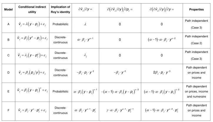
Drawing together sections 3.1 and 3.2, let us now consider the implications of the path independence conditions for the practical specification of RUM models. Table 1 introduces six specifications of the conditional indirect utility function; all have seen practical usage in the literature, although some more commonly than others. The first column of the table labels the models A to F, the second column gives the precise specification of conditional indirect utility that each model entails, and the third

column notes whether the model relates to the discrete-continuous demand or the probabilistic demand. The fourth column derives the conditional marginal utility of

income, whilst the fifth and sixth columns differentiate the conditional marginal utility of income with respect to price and income respectively. The final column summarises the properties of the model in terms of path independence (with particular reference to Cases 1, 2 and 3 discussed above).

Model A is McFadden’s (1981) ‘residual income’ form, which complies with Assumptions I to V detailed in section 2. Note furthermore that, since

j j j

v p v y

     for j 1,2, Roy’s identity (3) will yield conditional demands of

12

17

one unit for both goods 1 and 2, meaning that Model A is applicable to the context of probabilistic demand. With regards to the path independence conditions, note that

the conditional marginal utility of income is independent of prices and income. On this basis, we can reason that Model A is consistent with Case 3 of the path

independence conditions for the probabilistic demand; this is to say, if y p_j then

any income effects (associated with homothetic or quasi-linear preferences) can be capitalised in terms of the demand for the numeraire good.

Model B is a slight adjustment to Model A that introduces a power term on income, common to goods 1 and 2. If this power term is significantly different from one then income will have a non-linear effect on conditional indirect utility. Furthermore, since

j j j

v p v y

     for j 1,2, Roy’s identity will yield conditional demands that differ

from one, meaning that Model B is applicable to the context of discrete-continuous demand. Since Model B embodies path independence with respect to prices but path dependence with respect to income, we can reason that it is consistent with Case 2 of the path independence conditions for the discrete-continuous demand.

Model C also introduces a power term to Model A, but this time on price rather than income; again we assume that the power term is common to goods 1 and 2. If this power term is significant, then Model C will yield discrete-continuous demands for goods 1 and 2, whilst preserving the path independence properties of Model A. In other words, the conditional marginal utility of income is independent of prices and income, consistent with Case 3.

Model D specifies price as a ratio of income (see for example Hau (1985)). If y p_j

for j 1,2, this model will again yield discrete-continuous demands. In the case of

Model D, however, the conditional marginal utility of income is dependent upon the prices of both goods 1 and 2, and dependent upon income. The path independence conditions for the discrete-continuous demand are therefore violated.

18

admitted through the numeraire good. We conclude therefore that Model E is not theoretically valid.

Finally, Model F employs a Cobb-Douglas-type specification. If y p_j then this will

give rise to discrete-continuous demands. Furthermore, if the power terms are significant, then Model F will embody path dependence with respect to prices and income.

4. SUMMARY AND CONCLUSIONS

With reference to the three objectives introduced in section 1, we will finish by summarising the principal outcomes, and drawing conclusions.

In response to the first objective, we introduced the problem of discrete-continuous demand proposed by S&R, involving two mutually exclusive goods (goods 1 and 2) and a ‘numeraire’ good (good n). We discussed the derivation of consumer surplus from the discrete-continuous demand in general, and the discrete choice (or

probabilistic) demand in particular. We then considered the conditions under which a change in consumer surplus will be independent of the sequence of price and/or income changes. With regards to the discrete-continuous demand, we identified three such cases:

Case 1: Let the marginal utility of income be independent of the price of good 1 and income, i.e. 



p,y



 p₁ 0 and 

 

p,y  y 0. This case will give rise to an indifference map embodying quasi-linear preferences.

Case 2: Let the marginal utility of income be independent of the prices of goods 1 and 2, i.e. 

 

p,y  p_j 0 for j 1,2. This case will give rise to an indifference

map that exhibits homothetic preferences.

Case 3: Let the marginal utility of income be independent of the prices of goods 1 and 2 as well as the income share available to goods 1 and 2 (once the numeraire

19

 

,y y1 2 0

 

 p   . In this case, any income change will be entirely devoted to/abstracted from the numeraire good.

In response to the second objective of the paper, we noted that the probabilistic demand, which might be seen as a restriction upon the discrete-continuous demand, gives rise to S&R’s consumer surplus measure (7). This measure is underpinned by Assumptions I to V (section 2 above), which impose path independence to price changes a priori. On this basis, the paper devoted particular attention to Case 3, since this is the only case where changes in consumer surplus will (additionally) be

path independent to changes in income. More specifically, if _j



p y_j,



y_{1 2} 0 for

1,2

j  and a numeraire good is present in the consumption bundle then, with certain

qualifications (Marshall, 1920), S&R’s consumer surplus measure will be path independent to income changes as well as to price changes, whilst observing

homogeneity and adding-up.

In response to the third objective, we illustrated several specifications of the

conditional indirect utility function commonly applied in practice, and reconciled them with Cases 1, 2 and 3 above. With particular reference to the probabilistic demand, we showed that McFadden’s (1981) ‘residual income’ specification is an appropriate means of implementing Case 3.

ANNEX: DERIVATION OF THE DISCRETE-CONTINUOUS DEMAND

FUNCTION

In this annex, we will derive13 the Marshallian discrete-continuous demands for goods 1 and 2 from S&R’s (1981) consumption problem. Slightly adjusting (1), so as

to explicate the role of the numeraire good, S&R’s problem is given by:





 

 

1 2 1 1 2 2

1 2 1 2

Max , ,

s.t.

0

, , 0

n

n

n

u u x x x

p x p x x y

x x

x x x

  

  

 

(A1)

13

20

Using the Lagrangean method, (A1) translates to the following maximization problem:



1 2

 

1 1 2 2





1 2



Max Lu x x x, , _n  yp x p x x_n  x x (A2)

Differentiating (A2) for the first order conditions:

1 2 1 1

0

L u

p x

x x  

 _  _{  }

  (A3)

2 1 2 2

0

L u

p x

x x  

 _  _{  }

  (A4)

0

n n

L u

x x 

 _  _{ }

  (A5)

L y 

 _

 (A6)

1 1 2 2 n 0

yp x p x x  (A7)

1 2 0

x x  (A8)

As discussed in section 2, S&R conceptualise (A1) as a problem of discrete-continuous demand. The individual first chooses between goods 1 and 2 according to which yields the greater utility. Having made that choice, the individual then consumes a positive continuous quantity of only the chosen good. On this basis,

note that if x₁0, then x₂ 0, and (A4) will become redundant. If instead x₂ 0, then x₁0, and (A3) will become redundant. Motivated by this rationale, let us define the conditional indirect utility functions, which might be seen as an extension of (2):









 





1

1 1, 1 1 1, , n 1, _{x 0}

v p y u x p y x p y _ (A9)









 





2

2 2, 2 2 2, , n 2, _{x 0}

v p y u x p y x p y _ (A10)

21

be devoted to the numeraire good, and that the extent of this residual may be different depending on which good is chosen.

On the basis of (A9) and (A10), and making use of (A3) to (A6), we can restate the first order conditions in terms of the conditional indirect utility functions:

1 1

1

0 0

1 1 1 1 1

1 1

1 1 1 ₀ 1 1 1

n_x n_x

n x

x x

v u x u x

p

p x p x p  p p

           _  _    _  _

     _   _ (A11)

2 2

2

0 0

2 2 2 2 2

2 2

2 2 2 0 2 2 2

nx nx

n x

x x

v u x u x

p

p x p x p  p p

        _   _  _{ }  _{ }  

     _   _ (A12)

1 1

1

0 0

1 1 1 1 1

1 1

1 0

n_x n _x

n x

x x

v u x u x

p

y x y x y  y y

        _  _  _{ }  _{ }  

     _   _ (A13)

2 2

2

0 0

2 2 2 2 2

2 2

2 ₀

nx nx

n x

x x

v u x u x

p

y x y x y  y y

        _   _  _{ }  _{ }  

     _   _ (A14)

where the marginal utility of income is now conditioned by choice (see footnote 8),

hence the notation _j for j 1,2.

Given the budget constraint (A7), and again accounting for conditioning by choice, it must hold that:

1

1

0 1

1 1

1 0 1 1

0 n x x x y x x p

p p p

 



 _{ }  _{ }

   (A15)

2

2

0 2

2 2

2 0 2 2

0 n x x x y x x p

p p p

 



 

   

   (A16)

1 1 0 1 1 0 1 n x x x y x p

y y y

 



 _  _{ }

   (A17)

2 2 0 2 2 0 1 n x x x y x p

y y y

 



 _  _{ }

   (A18)

22 1 1 1 1 v x p   _{ }  (A19) 2 2 2 2 v x p   _{ }  (A20) 1 1 v y     (A21) 2 2 v y   _  (A22)

Equipped with (A19) to (A22), we can write Roy’s identity for the case of discrete -continuous consumption, and thereby derive the conditional demand for goods 1 and 2: 1 1 1 * 1 1 * 2 1 2 if 1

0 if 2 v p

x k

v y u p

u y v p

k v y              _{ }   _        (A23) 1 2 * 1 2 * 2 2 2 2

0 if 1

if 2 v p

k v y

u p

u y v p

x k v y              _{ }   _  _{ }     (A24)

Note that if we restrict (A1) to the context of a single discrete choice, then (A23) and

(A24) will elicit conditional demands x₁x₂ 1.

ACKNOWLEDGEMENTS

The authors gratefully acknowledge the comments of the peer reviewers, which significantly improved the clarity of the paper. Any remaining errors or limitations are of course the sole responsibility of the authors.

23

REFERENCES

Batley, R. & Ibáñez, J.N. (2013) ‘Applied welfare economics with discrete choice models: implications of theory for empirical specification’. In Hess, S. & Daly, A. (eds) Choice Modelling: The State of the Art and the State of Practice. Edward Elgar, Cheltenham.

Batley, R. (2013) ‘The intuition behind income effects of price changes in discrete

choice models, and a simple method for estimating the compensating variation’. Working Paper, Institute for Transport Studies, University of Leeds.

Block, H.D. & Marschak, J. (1960) ‘Random orderings and stochastic theories of

responses’. In Marschak, J. (1974) Economic Information, Decision and Prediction: Selected Essays (Volume 1). D. Reidel, Dordrecht.

Dagsvik, J.K. & Karlström, A. (2005) ‘Compensating variation and Hicksian choice probabilities in Random Utility Models that are non-linear in income’. The Review of Economic Studies, 72 (1), pp57-76.

Daly, A. & Zachary, S. (1978) ‘Improved multiple choice models’. In Hensher, D.A. and Dalvi, Q. (eds) Determinants of Travel Choice. Saxon House, Farnborough.

Deaton, A. & Muellbauer, J. (1980) Economics and Consumer Behavior. Cambridge University Press, Cambridge.

Gorman, W.M. (1953) ‘Community preference fields’. Econometrica, 21 (1), pp63-80.

Hanemann, W.M. (1982) Applied welfare analysis with qualitative response models.

CUDARE Working Paper 241, Department of Agricultural & Resource Economics, University of California, Berkeley.

Hanemann, W.M. (1999) ‘Welfare economics using discrete choice models’. In Kling, C. & Herriges, J. (eds) Valuing Recreation and the Environment: Revealed

Preference Methods in Theory and Practices. Edward Elgar, Cheltenham.

Hau, T.D. (1985) ‘A Hicksian approach to cost-benefit analysis with discrete choice

models’. Economica, 52 (208), pp479-490.

Hau, T.D. (1987) ‘Using a Hicksian approach to cost-benefit analysis in discrete

choice: an empirical analysis of a transportation corridor simulation model’.

24

Herriges, J.A. & Kling, C.L. (1999) ‘Nonlinear income effects in Random Utility

Models’. The Review of Economics and Statistics, 81 (1), pp62-72.

Ibáñez, J.N. & R. Batley (2011) ‘On the duality relations for discrete-continuous

demand where price is an indicator of quality’. Working paper, Institute for Transport Studies, University of Leeds.

Jara-Díaz, S.R. (1990) ‘Consumer’s surplus and the value of travel time savings’. Transportation Research Part B, 24 (1), pp73-77.

Jara-Díaz, S.R. & Farah, M. (1988) ‘Valuation of users’ benefits in transport systems’. Transport Reviews, 8 (3), pp197-218.

Jara-Díaz, S.R. & Videla, J. (1989) ‘Detection of income effect in mode choice:

theory and application’. Transportation Research Part B, 238 (6), pp393-403.

Jara-Díaz, S.R. & Videla, J. (1990) ‘Welfare implications of the omission of income

effect in mode choice models’. Journal of Transport Economics and Policy, 24 (1), pp83-93.

Johansson, P.O. (1987) The Economic Theory and Measurement of Environmental Benefits. Cambridge University Press, Cambridge.

Karlström, A. (1999) ‘Four essays on spatial modelling and welfare analysis’. Report TRITA-IP FR 99-49, Department of Infrastructure and Planning, Royal Institute of Technology.

Karlström, A. & Morey, E.R. (2001) ‘Calculating the exact compensating variation in

logit and nested-logit models with income effects: theory, intuition, implementation, and application’. Paper presented at the meeting of the American Economic

Association, New Orleans, January 2001.

McFadden, D., Tye, W. & Train, K. (1978) An application of diagnostic tests for the Independence from Irrelevant Alternatives property of the multinomial logit model, Transportation Research Record, 637, pp39-46.

25

McFadden, D.L. (1995) ‘Computing willingness-to-pay in Random Utility Models’. Working paper, Department of Economics, University of California, Berkeley.

Marschak, J. (1960) ‘Binary choice constraints and random utility indicators’. In

Marschak, J. (1974) Economic Information, Decision and Prediction: Selected Essays (Volume 1). D. Reidel, Dordrecht.

Marshall, A. (1920) Principles of Economics. Macmillan, London.

Samuelson, P.A. (1942) ‘Constancy of the marginal utility of income’. In Lange, O.,

McIntyre, F. & Yntema, T.O. (eds) Studies in Mathematical Economics and Econometrics in Memory of Henry Schultz. University of Chicago Press, Chicago.

[image:27.842.61.785.88.503.2]

26

Table 1: Some common practical model specifications, and their properties in terms of path independence

Model Conditional indirect utility

Implication of

Roy’s identity vj  y  



vj y



 pj  



vj y



 y Properties

A v_j 



y p_j



_j Probabilistic  0 0

Path independent (Case 3)

B vj j



y pj



j



 

  

Discrete-continuous

1

j y



 _{ } 

0



  1



 _j y2 Path independent (Case 2)

C v_j _j



yp_j



_j

Discrete-continuous j 0 0

Path independent (Case 3)

D v_j _j



p y_j



_j Discrete-continuous

2

j p yj

 

   2

j y

 

  3

2_jp y_j  

Path dependent on prices and

income

E vj j



y pj



j



 

   _{Probabilistic}

_

_

1

j y pj



   









2

1 _j y p_j 

   

    









2

1 _j y p_j 

     

Path dependent on prices, income

and numeraire

F v_j _j yp_j _j Discrete-continuous

1

j y pj

 

 _{ }  _ 1 1

j y pj

 

  _{  }  _ 



₁



2

j y pj

 

_{  }  _  _

Path dependent on prices and