This is a repository copy of
The Gradient Free Directed Search Method as Local Search
within Multi-objective Evolutionary Algorithms
.
White Rose Research Online URL for this paper:
http://eprints.whiterose.ac.uk/98449/
Version: Accepted Version
Proceedings Paper:
Lara, A., Alvarado, S., Salomon, S. et al. (3 more authors) (2013) The Gradient Free
Directed Search Method as Local Search within Multi-objective Evolutionary Algorithms. In:
EVOLVE - A Bridge between Probability, Set Oriented Numerics, and Evolutionary
Computation II. EVOLVE 2012, 07-09 Aug 2012, Mexico City. Advances in Intelligent
Systems and Computing (175). Springer Berlin Heidelberg , p. 153. ISBN
978-3-642-31518-3
https://doi.org/10.1007/978-3-642-31519-0_10
[email protected] https://eprints.whiterose.ac.uk/
Reuse
Unless indicated otherwise, fulltext items are protected by copyright with all rights reserved. The copyright exception in section 29 of the Copyright, Designs and Patents Act 1988 allows the making of a single copy solely for the purpose of non-commercial research or private study within the limits of fair dealing. The publisher or other rights-holder may allow further reproduction and re-use of this version - refer to the White Rose Research Online record for this item. Where records identify the publisher as the copyright holder, users can verify any specific terms of use on the publisher’s website.
Takedown
If you consider content in White Rose Research Online to be in breach of UK law, please notify us by
as Local Search within Multi-Objective
Evolutionary Algorithms
Adriana Lara, Sergio Alvarado, Shaul Salomon, Gideon Avigad, Carlos A. Coello Coello, and Oliver Sch¨utze
Abstract.Recently, the Directed Search Method has been proposed as a point-wise iterative search procedure that allows to steer the search, in any direction given in objective space, of a multi-objective optimization problem. While the original version requires the objectives’ gradients, we consider here a possible modifica-tion that allows to realize the method without gradient informamodifica-tion. This makes the novel algorithm in particular interesting for hybridization with set oriented search procedures, such as multi-objective evolutionary algorithms.
In this paper, we propose the DDS, a gradient free Directed Search method, and make a first attempt to demonstrate its benefit, as a local search procedure within a memetic strategy, by integrating the DDS into the well-known algorithm MOEA/D. Numerical results on some benchmark models indicate the advantage of the result-ing hybrid.
1
Introduction
Many real world problems demand for the concurrent optimization ofkobjectives
leading to amulti-objective optimization problem(MOP) [16]. One characteristic
of these problems, compared with those where only oneobjective is under
con-sideration, is that the solution set of a MOP (the Pareto set) typically forms a
Adriana Lara
Mathematics Department ESFM-IPN, Edif. 9 UPALM, 07300 Mexico City, Mexico
e-mail:[email protected]
Sergio Alvarado·Carlos A. Coello Coello·Oliver Sch¨utze
Computer Science Department, CINVESTAV-IPN, Av. IPN 2508, Col. San Pedro Zacatenco, 07360 Mexico City, Mexico
e-mail:{ccoello,schuetze}@cs.cinvestav.mx,
Shaul Salomon·Gideon Avigad
ORT Braude School of Engineering, Karmiel, Israel
e-mail:{shaulsal,gideona}@braude.ac.il
(k−1)-dimensional object. So far, there exist many methods for the computation of the Pareto set of a MOP. Among them, multi-objective evolutionary algorithms (MOEAs) have caught the attraction of many researchers (e.g., [7, 6] and references therein). The major reason for this might be that the population based approach, together with a stochastic component in the search procedure, allows typically for an approximation of the entire (global) Pareto set in one single run of the algo-rithm. This represents an advantage over most mathematical programming (MP) techniques, which require in addition certain smoothness assumptions on the MOP. On the other hand, it is well-known that MOEAs normally need a large amount of function evaluations, due to their slow convergence rate, in order to generate a suit-able finite size approximation of the set of interest ([4]). As a remedy, researchers
have proposedmemetic MOEAs, i.e., hybrids of MOEAs and MP with the aim to
get fast and reliable global search procedures (e.g., [9, 11, 10, 22, 14]).
In this paper, we adapt the Directed Search (DS) method [21] for the use within MOEAs. One crucial drawback of the DS is that it requires gradient information which restricts its usability. Here, we propose a modification of the DS that is gradi-ent free. Even more, the computation of the search direction comes without the cost of additional function evaluations if the neighborhood information can be exploited. The latter makes the Discrete Directed Search (DDS) a suitable algorithm, in partic-ular, for the usage within set oriented search techniques. We demonstrate the benefit of the DDS by hybridizing it with MOEA/D ([24]), a state-of-the-art MOEA whose neighborhood definition can be directly used for the DDS.
The remainder of this paper is organized as follows: In Section 2, we give the re-quired background for the understanding of the sequel. In Section 3, we present the DDS, a gradient free Directed Search variant. In Section 4, we propose a way to integrate the DDS into MOEA/D leading to a new memetic algorithm. In Section 5, we present some results, and finally, we draw our conclusions in Section 6.
2
Background
In the following we consider unconstrained multi-objective optimization problems (MOPs) which can be stated as follows:
min
x∈Ê
nF(x), (1)
whereF :R⊂Ê
n→
Ê
k is defined as the vector ofkobjective functions f
i:R⊂
Ê
n→
Ê,i=1, . . . ,k. A pointx∈Ris said to dominate another point y∈R, if fi(x)≤ fi(y)for alli∈ {1, . . . ,k}, and if there exists an index j∈ {1, . . . ,k}such
thatfj(x)<fj(y). A pointx∈Ris called optimal, orParetooptimal, with respect to
(1), if there is no other pointy∈Rthat dominatesx. The set of all optimal solutions
is called the Pareto set, and the set of images of the optimal solutions is called the the Pareto front.
Recently, a numerical method has been proposed for differentiable MOPs that
allows to steer the search from a given point into a desired direction d ∈Ê
objective space ([21]). To be more precise, given a pointx∈Ê
n, a search direction
ν∈Ê
nis sought such that
lim
tց0
fi(x0+tν)−fi(x0)
t =di, i=1, . . . ,k. (2)
Such a direction vectorνsolves the following system of linear equations:
J(x0)ν=d, (3)
whereJ(x)denotes the Jacobian ofF atx. Since typicallyk<<n, we can assume
that the system in Equation (3) is (highly) underdetermined. Among the solutions of Equation (3), the one with the smaller 2-norm can be viewed as the greedy direction for the given context. This solution is given by
ν+:=J(x)+d, (4)
whereJ(x)+denotes the pseudo inverse ofJ(x)(we refer e.g. to [17] for an efficient
computation ofν+). If one proceeds the search in directiond in the same manner,
this is identical to the numerical solution of the following initial value problem
(starting from solutionx0∈Ê
n):
x(0) =x0∈Ê
n
˙
x(t) =ν+(x(t)), t>0 (5)
Ifdis a ‘descent direction’ (i.e.,di≤0 for alli=1, . . . ,kand there exists an index
j such thatdj<0), a numerical solution of (5) can be viewed as a particular hill
climber for MOPs.
The endpointx∗of the solution curve of (5) does not necessarily have to be a
Pareto point, but it is a boundary point in objective space, i.e.,F(x∗)∈∂F(Ê
n)
which means that the gradients of the objectives inx∗are linear independent (and
hence, thatrank(J(x∗))<k). This fact can be used to check numerically if a current
iterate is near to a boundary point: For the condition number of the Jacobian it holds
κ2(J(x)) =
%
λmax(J(x)TJ(x))
λmin(J(x)TJ(x))→∞ for x→x
∗, (6)
whereλmax(A)andλmin(A)denote the largest and the smallest eigenvalue of matrix
A, respectively. (Roughly speaking, the condition number indicates how ‘near’ the
rows ofJ(x), i.e., the gradients of the objectives, are to be linearly independent: the
higher the value ofκ2(J(x)), the closerJ(x)is to a matrix with rank less thank.)
Further, one can check the (approximated) endpointx∗numerically for optimality
by checking if∑ki=1α˜i∇fi(x∗)2≤tol, wheretol>0 is a given tolerance and ˜α
min α ⎧ ⎨ ⎩ ) ) ) ) ) k
∑
i=1
αi∇fi(x)
) ) ) ) ) 2 2
: αi≥0,i=1, . . . ,k, k
∑
i=1
αi=1
⎫ ⎬ ⎭
(7)
The hill climber described above shares many characteristics with the one described
in [3], where also possible choices fordare discussed.
3
Gradient Free Directed Search
The key of the DS is to solve Equation (3) in order to find a vectorν such that
the search can be steered ind-direction. For this, the most expensive part might be
the computation or approximation of the objectives’ gradients. Here, we suggest an
alternative way to compute such search directionsνusing a finite difference method
tailored to the given context. We note that this approach is not equal to the classical finite difference approach used to approximate the gradient (e.g., [17]).
Assume we are given a candidate solutionx∈Ê
nandrsearch directionsν
i∈Ê
n,
i=1, . . . ,r. Define the matrixF(x)∈Ê
k×ras follows:
F(x):= (∇fi(x),νj) i=1, . . . ,k; j=1, . . . ,r. (8)
That is, every entrymi jofF is defined by the directional derivative of objectivefiin
directionνj,mi j=∇νjfi(x). Crucial for the subsequent discussion is the following
result:
Proposition 1 Let x,νi, i=1, . . . ,r∈Ê
n,λ∈
Ê
r, andν:=∑r
i=1λiνi. Then
J(x)ν=F(x)λ (9)
Proof. It is
F(x)λ =
⎛ ⎜ ⎝
∇f1(x),ν1 . . . ∇f1(x),νr
..
. ... ...
∇fk(x),ν1 . . . ∇fk(x),νr
⎞ ⎟ ⎠ ⎛ ⎜ ⎝ λ1 .. . λr ⎞ ⎟ ⎠ (10) and
J(x)ν=J(x)(
r
∑
i=1 λiνi) =
r
∑
i=1 λi
⎛ ⎜ ⎝
∇f1(x)T .. .
∇fk(x)T
⎞ ⎟
⎠νi (11)
Hence, for thel-th component of both products it holds
(F(x)λ)l= r
∑
i=1
λi∇fl(x),νi= (J(x)ν)l, (12)
Hence, in search for a directionν, one can instead of Equation (3) try to solve the following equation:
F(x)λ =d, (13)
and set
ν:=
r
∑
i=1
λiνi. (14)
Remark 1 Assume that we are given a candidate solution x0∈Ê
n and further r
points xi, i=1, . . . ,r, in the neighborhood of x0together with their function values F(xi), i=0, . . . ,r. Defining
νj:= xj−x0
xj−x02
, tj:=xj−x02, j=1, . . . ,r, (15)
one can approximate the entries ofF by finite differences as follows:
mi j=∇fi(x0),νj=lim tց0
fi(x0+tνj)−fi(x0) t
≈ fi(xj)−fi(x0) xj−x02
, i=1, . . . ,k, j=1, . . . ,r.
(16)
Analog to the well-known forward differences to approximate the gradient, one can show that the computational error is given by
∇fi(x0),νj=
fi(xj)−fi(x0) xj−x02
+O(xj−x02). (17)
Note that, by this, the search direction can be computed without any additional function evaluations.
Since it is ad hoc not clear if Equation (13) has a solution, and even if it is solvable,
how the condition of the problem is (in terms ofκ2(F)), we have to investigate the
choice ofrand theνi’s. For this, it is advantageous to writeF(x)as follows:
F(x) =J(x)V, (18)
whereV:= (ν1, . . . ,νr)∈Ê
n×ris the matrix consisting of the search directionsν
i.
If rank(J(x)) =k(which is given for a non-boundary pointx), it is known from
linear algebra that
rank(J(x)) =k ⇒ rank(F(x)) =rank(V). (19)
If on the other handxis a boundary point (and hence,rank(J(x))<k), then it follows
by the rank theorem of matrix multiplication that alsorank(F(x))<kregardless
of the choice ofV (i.e., regardless of the numberr and the choice of the search
This indicates that the condition number ofF(x)can be used to check
numeri-cally if a current iterate is already near to an endpoint of (5). Equation (19) indicates
that theνi’s should be chosen such that they are linearly independent. If in
addi-tion the search direcaddi-tions are orthogonal to each other, a straightforward calculaaddi-tion shows that
V orthogonal ⇒ κ2(F(x)) =κ2(J(x)). (20)
In that case, the condition numberκ2(F(x))can indeed be used as a stopping
crite-rion, analog to the original method described in Section 2. That is, one can stop the
iteration if for a current iteratexiit holds
κ2(F(xi))>tolκ, (21)
wheretolκ>>1 is a large number.
Example 1 Consider the following bi-objective model ([12]):
F:Ê
n→
Ê 2
fi(x) =x−ai22, i=1,2,
(22)
where a1= (1, . . . ,1)T,a2= (−1, . . . ,−1)T∈Ê
n. The Pareto set is given by the line
segment between a1and a2, i.e.,
P={x∈Ê
n
: xi=2α−1,i=1, . . . ,k,α ∈[0,1]} (23)
Let r=2and v1:=eiand v2:=ej, i=j, where eidenotes the i-th canonical vector.
Then, it is
F(x) =
xi−1 xj−1
xi+1 xj+1
(24)
It isdet(F(x)) =1/(2(xi−xj)), and hence,
det(F(x)) =0 ⇔ xi=xj, (25)
by which it follows that it is rank(F(x)) =2for all x∈Ê
n\B, where B:={x∈
Ê
n : x
i=xj}(note thatP⊂B). Since B is a zero set inÊ
n, the probability is one
that for a randomly chosen point x∈Ê
nthe matrixF(x)has full rank, and hence,
that Equation (13) has a unique solution. To be more precise, it isν=λ1ei+λ2ej,
where
λ =F−1(x)d= 1
det(F(x))
xj+1 −xj+1
−xi−1 xj−1
d1 d2
= 1
2(xi−xj)
xj(d1−d2) +d1+d2 xi(d2−d1)−d1−d2
.
(26)
The above considerations show that already for r =k search directions νi, i=1, . . . ,r, one can find a descent direction ˜νby solving Equation (13). However,
by construction it isν∈span{ν1, . . . ,νk} which means that only ak-dimensional
subspace of theÊ
nis explored in one step. One would expect that the more search
directionsνiare taken into account, the better the choice of ˜νis. This is indeed the
case: Forr>k, we suggest to choose analog to (4)
ν+(r):=
r
∑
i=1
λiνi, where λ=F(x0)+d (27)
The following discussion gives a relation between ν+(r) andν+ for non-boundary
pointsxfor the case that theνi’s are orthonormal: It is
ν+=J+(x)d=J(x)T(J(x)J(x)T)−1d (28)
and
λ=F(x)+d=VTJ(x)T(J(x)VVT
/ 012
I
J(x)T)−1d
=VTJ(x)T(J(x)J(x)T)−1d
/ 01 2
ν+
=VTν+ (29)
and hence
ν+(r)=
r
∑
i=1 λiνi=
r
∑
i=1
νi,ν+νi (30)
For instance, when choosingνi=eji, Equation (30) gets simplified:
ν+(r)=
r
∑
i=1 ν+,j
ieji, (31)
i.e.,ν+(r)has onlyrentries which are identical to the corresponding entries ofν+.
In both cases ν+(r) gets closer toν+ with increasing numberr and forr=n it is
ν+(r)=ν+.
Remark 2 We would like to stress that this approach is intended formulti-objective optimization problems (i.e., k>1). For the special (and important) case of scalar optimization (i.e., k=1), the present approach is of very limited value as the fol-lowing discussion shows: For r=k=1, Equation (13) reads as
∇f(x),ν1λ=d (32)
λ=
3
−1 if∇f(x),ν1>0
1 if∇f(x),ν1<0 (33)
and thus toν∈ {ν1,−ν1}. However, this does not bring any new insight: It is well-known that the descent cone of f at x is given by
C(x):={ν∈Ê
n
: ∇f(x),ν<0}, (34)
and hence, it is under the above assumption onν1eitherν1∈C(x)or−ν1∈C(x).
Finally, we state the Discrete Directed Search (DDS) which is simply a line search
along the search directionν+(r) (see Algorithm 1). For an efficient step size control
we refer to [15].
Algorithm 1Discrete Directed Search (DDS) Require: Initial solutionsx0,x1, . . .xr∈Ê
n
Ensure: New candidate solutionxnew
1: computeν+(r)as in Eq. (27).
2: computet∈Ê+
3: xnew:=x0+tν+(r)
4
Integration of DDS into MOEA/D
Here we show the potential of the DDS as local search engine within the state-of-the-art method MOEA/D [24]. The philosophy behind this MOEA consists of employing a decomposition approach, to convert the problem of approximating the Pareto front into a certain number of scalar optimization problems (SOPs). We stress that MOEA/D is indeed particularly attractive to be combined with the DDS proce-dure. Two important reasons for this are (a) MOEA/D has an implicit neighborhood structure, imposed by the particular decomposed problems, and (b) there is a weight vector associated to each subproblem, and to each individual.
In this sense, DDS can take advantage of (a) to avoid the computation of the
neighbors used to estimate the search direction ν+(r); also, no extra function
eval-uations are necessary, which makes the computation of the search direction an ef-fortless procedure—in terms of function evaluations. In other words, given a point x∈Ê
n,if some neighbors ofx
1, . . . ,xrare already evaluated, the computation can
be done without any additional function evaluations. In general, memetic MOEAs which use gradient-based information have already proven their efficacy on several MOPs [14, 3], but the cost of estimating the first order information has been always an issue.
for the movement performed by DDS. Furthermore, DDS also takes advantage that MOEA/D already has a computed reference point for the decomposed problems. In
this sense, once the individual p is chosen to be affected by the local search, the
values fordi in the DDS are already set for p (according with its corresponding
decomposed MOEA/D subproblem).
How to apply the local search is one of the main issues when designing memetic algorithms. Two important parameters have been identified [8, 13] as crucial when controlling the local search application on memetic MOEAs. They are:
(i) The frequencyklsfor application of the local search along the total amount of
generations.
(ii) The number of elementshls, from the population, to which the local search is
applied each generation.
Algorithm 2 describes the coupling of DDS and MOEA/D. The notation regarding MOEA/D procedures and parameters is consistent with the one presented in [24]. The SOP regarding the decomposition was, in this case, taken by the Tchebycheff approach as:
minimizegte(x|λ,z∗) = max
1≤i≤m{
λi|fi(x)−z∗i} (35)
wherez∗,such thatz∗i =min{fi(x)|x∈P0},is the reference point; and the direction
difor the application of DDS to the individualxiis set asdi=λi−z∗.
Algorithm 2MOEA/D/DDS
1: Set the weight vectorsλiand the neighborhoodsB(i) ={i1, . . . ,iT}for each
decomposed problem (λi1, . . . ,λiT are theTclosest weight vectors toλi).
2: Initialize an initial populationP0={x1, . . .xN}.
3: Initialize the reference pointz∗,EP=/0,gen=1.
4: repeat
5: fori=1, . . . ,Ndo
6: Select two indexesk,lfromB(i)and generate, using genetic operators, a new
solutionyfromxkandxl.
7: Apply the subproblem improvement heuristic for eachyin order to gety′
(Eq. 35).
8: ifmod(gen,kls) ==0 andmod(i,hls) ==0 then
9: Apply DDS toy′,in order to gety′′.
10: Sety′←y′′.
11: end if
12: Update the reference pointz∗.
13: Remove fromEPall the vectors dominated byy′and add it if no vectors inEP
dominatey′.
14: end for
15: gen=gen+1.
16: untilStopping criteria is satisfied
5
Numerical Results
In this section we show some results of the MOEA/D/DDS for the computation of Pareto fronts as well as of the DS in the context of a particular control problem.
5.1
Comparison MOEA/D and MOEA/D/DDS
Since we have chosen MOEA/D as base MOEA, it seems reasonable to test over the CEC09 benchmark [27]. For this, we adapted the available code from a specific version of MOEA/D [25], which was tested for performance with remarkable results over this particular test suite [26]. Differences of this code and the MOEA/D original version are that this modification allows the computational effort to be distributed
among the subproblems based on an utility functionπidefined for each subproblem.
The main parameters for MOEA/D were set according to Table 1, and for the
DDS we have chosenr=5. We stop the computations after 30,000 function
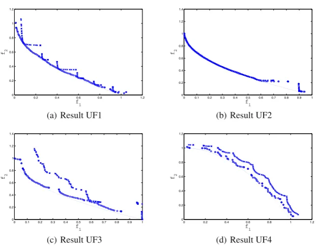
eval-uations, which represents the 10% of the budget originally allowed by the compe-tition. Figure 1 presents plots that show that the Pareto front has been reached, by the MOEA/D/DDS using this reduced budget. Finally, the parameters related to the control for application of the local search are presented in Table 2. As performance indicators to compare the results of the different algorithms we have chosen to take the Generational Distance (GD, see [23]), the Inverted Generational Distance (IGD,
see [5]), the averaged Hausdorff Distance∆1(see [19, 20]) which is in fact the
max-imum of the GD and the IGD value, and the Hypervolume indicator (HV, see [28]). From Figure 1 and Table 3 it becomes clear that the new hybrid is outperforming its base MOEA in three out of four cases. For UF2, the indicator values of MOEA/D are slightly better, however, there is no clear winner.
Table 1 Parameters setting for MOEA/D in this experiments
Identifier Value Description
N 600 The number of subproblems considered
T 0.1 N Size of the neighborhood
Pm 1/n Mutation rate
EP 100 Number of final solutions (external population)
Table 2 Parameters setting for the memetic part
Identifier Value Description
kls (0.15) tg Local search application frequency; tg is the total number of generations. hls (0.1) N Percentage of the population over which the
0 0.2 0.4 0.6 0.8 1 1.2 0 0.2 0.4 0.6 0.8 1 1.2 f1 f2
(a) Result UF1
0 0.1 0.2 0.3 0.4 0.5 0.6 0.7 0.8 0.9 1 0 0.2 0.4 0.6 0.8 1 1.2 1.4 f1 f2
(b) Result UF2
0 0.1 0.2 0.3 0.4 0.5 0.6 0.7 0.8 0.9 1 0 0.2 0.4 0.6 0.8 1 1.2 1.4 f 1 f2
(c) Result UF3
0 0.2 0.4 0.6 0.8 1 1.2
0 0.2 0.4 0.6 0.8 1 1.2 f 1 f2
(d) Result UF4
[image:12.429.58.369.79.322.2]Fig. 1 Numerical results for MOEA/D (crosses) and MOEA/D/DDS (circles) on the bench-mark models UF1 to UF4 (compare also to Table 3). The true Pareto fronts are indicated by the dotted lines.
Table 3 Indicator values obtained by MOEA/D and MOEA/D/DDS on the benchmark
mod-els UF1 to UF4. The budget for the function evaluations was set to 30,000. The information
was gathered by 10 independent runs.
Indicators
Problems GD IGD ∆1 HV
UF1 MOEA/D
MOEA/D/DDS
0.0696046570
0.0415884479
0.0709107497
0.0400041235
0.0736649773
0.0422788829
0.9431136545
0.9619027643
UF2 MOEA/D
MOEA/D/DDS
0.0261457333
0.0323564751
0.0195839746
0.0151025484
0.0261457333
0.0323564751
0.9757865917
0.9645998451
UF3 MOEA/D
MOEA/D/DDS
0.1459679411
0.0552610854
0.1307335754
0.0537723289
0.1520909424
0.0616385221
0.8604675543
0.9608503276
UF4 MOEA/D
MOEA/D/DDS
0.0823081769
0.0472797997
0.0871159952
0.0472797997
0.0871159952
0.0478409975
0.9206159284
[image:12.429.55.375.428.538.2]5.2
A Control Problem
The skill of the DS is to steer the search into any direction in objective space. This can be used for Pareto front computations as seen above, however, may also have other applications as the following discussion shows. In [1], robustness of optimal solutions to MOPs subject to physical deterioration has been addressed. The prob-lem posed in that study involves the need to steer the decorated performances (due to undesired changes in some design parameters) as close as possible to the origi-nal performances. In order to elucidate this demand for robustness, consider a two
parameter bi-objective design space (i.e.,n=k=2). Assume Figure 2 shows four
optimal solutions, and that the performance vector designated by the bold circle is
the decision makers selected solution (denote byx∗). Now suppose that due to wear,
one of the design parameters associated with that solution, changes (sayx1). This
will cause the performances to deteriorate (see the triangle in both panels). Now
sup-pose that there is a way to actively change the remaining parameterx2by actively
controlling its value. If this is done properly, the performances might be improved to new performance vectors (designated in the figures by squares). The way the de-teriorated performances are steered (controlled) as close as possible to the original
location, has been termed in [1] as ‘control in objective space’. In [1] the control
0 1 2 3 4 5 6
0 1 2 3 4 5 6
x1
x2
(a) Parameter space
0 1 2 3 4 5 6
0 1 2 3 4 5 6
f1
f2
(b) Image space
Fig. 2 Hypothetical two dimensional bi-objective design problem
problem has been defined as a regulative control problem, and a proportional con-troller has been used to update the optimal solution in time. Note, however, that since optimality is defined in objective space, the DS (or DDS) can be used to
ac-complish this task: The directiondiis simply the difference of performance of the
[image:13.429.272.372.306.425.2]To illustrate the performance of the suggested control scheme, we choose the quadratic bi-objective problem
F:Ê 15→
Ê 2
F(x) = (x−a122,x−a222),
(36)
where a1= (1, . . . ,1)anda2= (−1, . . . ,−1). For the decision space we choose
n=15 whereof three parameters deteriorate (x1,x2, andx3) and the rest can be
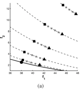
con-trolled. The results for the handling of the DDS controller with the above problem are depicted in Figure 3 (a). The solid line represents the initial Pareto front. The circle is the performance of the initial design. The performance after deterioration occurs is marked with triangles. Since some design variables have deteriorated, the Pareto front has changes in time. The deteriorated Pareto front in every time step is marked with a dashed line. The final state of the DDS controlled performance is marked with a black square, while the trajectory is marked with smaller gray squares. Note that the trajectory is going along the Pareto optimal front, and stops when the error is minimal. Figure 3 (b) depicts the performance of the deteriorated product with and without the DDS controller. The uncontrolled performance is de-scribed with triangles and the controlled one with squares.
We note that this result has been obtained by using the classical DS, however, from this we conclude that the DDS might be an alternative choice for models where no gradient information is at hand. We leave this for future research.
36 38 40 42 44 46 48
2 4 6 8 10 12
f1
f2
(a)
40 45 50 55 60
5 10 15 20 25
f1
f2
(b)
[image:14.429.53.185.347.491.2]6
Conclusions
In this paper, we have modified the Directed Search Method, a point-wise iterative search procedure that allows to steer the search into any direction given in objective space of a given MOP. The resulting algorithm, DDS, allows to perform similar iter-ations as its original, however, without using gradient information but by exploiting the neighborhood information in order to find a suitable search direction. The latter makes the new algorithm in particular interesting for set oriented search procedures such as MOEAs. Here, we have made a first attempt to demonstrate this by inte-grating the DDS into MOEA/D. Comparisons on some benchmark functions have shown the benefit of such a hybridization.
For future work, the development of more efficient memetic strategies as the one proposed in this paper is an interesting topic which will call for a more sophisticated interplay of local and global search. Also, the adaption of the DDS to higher dimen-sional problems seems to be very interesting. Note that the choice of the number of
test points near a solutionx0that have to be chosen in order to find a search direction
merely depends on the number of objectives involved in the MOP, and not on the dimension of the parameter space. Finally, we intend to utilize the DS/DDS in other applications, e.g., in the context of changing market demands as described in [2].
Acknowledgements. This research was supported by a Marie Curie International Research Staff Exchange Scheme Fellowship within the 7th European Community Framework Pro-gram. The first author acknowledges support from IPN project no. 20121478, and the last author acknowledges support from CONACyT project no. 128554.
References
1. Avigad, G., Eisenstadt, E.: Robustness of Multi-objective Optimal Solutions to Physical Deterioration through Active Control. In: Deb, K., Bhattacharya, A., Chakraborti, N., Chakroborty, P., Das, S., Dutta, J., Gupta, S.K., Jain, A., Aggarwal, V., Branke, J., Louis, S.J., Tan, K.C. (eds.) SEAL 2010. LNCS, vol. 6457, pp. 394–403. Springer, Heidelberg (2010)
2. Avigad, G., Eisenstadt, E., Sch¨utze, O.: Handling changes of performance-requirements in multi objective problems. Journal of Engineering Design (to appear, 2012)
3. Bosman, P.A.N., de Jong, E.D.: Exploiting gradient information in numerical multi-objective evolutionary optimization. In: Beyer, H.-G., et al. (eds.) 2005 Genetic and Evolutionary Computation Conference (GECCO 2005), vol. 1, pp. 755–762. ACM Press, New York (2005)
4. Brown, M., Smith, R.E.: Directed multi-objective optimisation. International Journal of Computers, Systems and Signals 6(1), 3–17 (2005)
5. Coello Coello, C.A., Cruz Cort´es, N.: Solving Multiobjective Optimization Problems using an Artificial Immune System. Genetic Programming and Evolvable Machines 6(2), 163–190 (2005)
6. Coello Coello, C.A., Lamont, G.B., Van Veldhuizen, D.A.: Evolutionary Algorithms for Solving Multi-Objective Problems, 2nd edn. Springer, New York (2007)
8. Ishibuchi, T.Y.H., Murata, T.: Balance between Genetic Search and Local Search in Hy-brid Evolutionary Multi-Criterion Optimization Algorithms. In: Proceedings of the Ge-netic and Evolutionary Computation Conference (GECCO 2002), pp. 1301–1308. Mor-gan Kaufmann Publishers, San Francisco (2002)
9. Ishibuchi, H., Murata, T.: Multi-objective genetic local search algorithm. In: Proc. of 3rd IEEE Int. Conf. on Evolutionary Computation, Nagoya, Japan, pp. 119–124 (1996) 10. Jaszkiewicz, A.: Do multiple-objective metaheuristics deliver on their promises? a
com-putational experiment on the set-covering problem. IEEE Transactions on Evolutionary Computation 7(2), 133–143 (2003)
11. J.: D Knowles and D.W Corne. M-PAES: a memetic algorithm for multiobjective
optimization. In: Proceedings of the IEEE Congress on Evolutionary Computation, Pis-cataway, New Jersey, pp. 325–332 (2000)
12. K¨oppen, M., Yoshida, K.: Many-Objective Particle Swarm Optimization by Gradual Leader Selection. In: Beliczynski, B., Dzielinski, A., Iwanowski, M., Ribeiro, B. (eds.) ICANNGA 2007. LNCS, vol. 4431, pp. 323–331. Springer, Heidelberg (2007)
13. Lara, A., Coello Coello, C.A., Sch¨utze, O.: A painless gradient-assisted multi-objective memetic mechanism for solving continuous bi-objective optimization problems. In: 2010 IEEE Congress on Evolutionary Computation (CEC), pp. 1–8. IEEE, IEEE Press (2010) 14. Lara, A., Sanchez, G., Coello Coello, C.A., Sch¨utze, O.: HCS: A new local search strat-egy for memetic multiobjective evolutionary algorithms. IEEE Transactions on Evolu-tionary Computation 14(1), 112–132 (2010)
15. Mejia, E., Sch¨utze, O.: A predictor corrector method for the computation of boundary points of a multi-objective optimization problem. In: International Conference on Electri-cal Engineering, Computing Science and Automati Control (CCE 2010), pp. 1–6 (2007) 16. Miettinen, K.M.: Nonlinear Multiobjective Optimization. Springer (1999)
17. Nocedal, J., Wright, S.: Numerical Optimization. Springer Series in Operations Research and Financial Engineering. Springer (2006)
18. Sch¨affler, S., Schultz, R., Weinzierl, K.: A stochastic method for the solution of un-constrained vector optimization problems. Journal of Optimization Theory and Applica-tions 114(1), 209–222 (2002)
19. Schuetze, O., Equivel, X., Lara, A., Coello Coello, C.A.: Some comments on GD and IGD and relations to the Hausdorff distance. In: GECCO 2010: Proceedings of the 12th Annual Conference Comp. on Genetic and Evolutionary Computation, pp. 1971–1974. ACM, New York (2010)
20. Sch¨utze, O., Esquivel, X., Lara, A., Coello Coello, C.A.: Using the averaged Hausdorff distance as a performance measure in evolutionary multi-objective optimization. IEEE Transactions on Evolutionary Computation (2012), doi:10.1109/TEVC.2011.2161872 21. Sch¨utze, O., Lara, A., Coello Coello, C.A.: The directed search method for unconstrained
multi-objective optimization problems. In: Proceedings of the EVOLVE – A Bridge Be-tween Probability, Set Oriented Numerics, and Evolutionary Computation (2011) 22. Vasile, M.: A behavior-based meta-heuristic for robust global trajectory optimization. In:
IEEE Congress on Evolutionary Computing, vol. 2, pp. 494–497 (2007)
23. Van Veldhuizen, D.A.: Multiobjective Evolutionary Algorithms: Classifications, Analyses, and New Innovations. PhD thesis, Department of Electrical and Computer En-gineering. Graduate School of EnEn-gineering. Air Force Institute of Technology, Wright-Patterson AFB, Ohio (May 1999)
25. Zhang, Q., Liu, W., Li, H.: The performance of a new version of moea/d on cec09 un-constrained mop test instances. In: IEEE Congress on Evolutionary Computation, CEC 2009, pp. 203–208. IEEE (2009)
26. Zhang, Q., Suganthan, P.N.: Final report on CEC09 MOEA competition. In: Congress on Evolutionary Computation, CEC 2009 (2009)
27. Zhang, Q., Zhou, A., Zhao, S., Suganthan, P.N., Liu, W., Tiwari, S.: Multiobjective op-timization test instances for the cec 2009 special session and competition. University of Essex, Technical Report (2008)