A learning framework for higher-order consistency models in multi-class pixel labeling problems

(1)

Higher-Order Consistency Models

in Multi-class Pixel Labeling

Problems

Kyoungup Park

A thesis submitted for the degree of

Doctor of Philosophy

The Australian National University

(2)

(3)

Except where otherwise indicated, this thesis is my own original work.

Kyoungup Park

(4)

(5)

(6)

(7)

I express my greatest gratitude to my supervisor Stephen Gould. Without his guide to this research, I could not see this honorable moment in my life. He has inspired me to keep continuing my research and provided valuable advices whenever I was lost in my direction. He is diligent and passionate as a mentor, and patient to listen to me and wait for my progress. I have learned from you so much about how to solve challenging problems in research. My thesis has benefitted greatly from you.

I am also grateful to my supervisor, Hongdong Li. As a panel chair, he has continued to offer guidance and support me in my research. He helped deal with an academic schedule given to me, and allowed me to use my time and resource as much as I wanted, which made it possible for me to finish this research. I appreciate your putting trust in me.

I would like to thank my supervisor Yi Li for providing valuable support and advice. He provided me the great research environment in NICTA and help me to continue my work. His concern and care about me in NICTA was helpful to drive my loneliness away. NICTA is a comfortable place to do research, where I could conduct my experiments using large scale servers freely.

Furthermore, I would like to thank Professor Richard Hartley for serving on my supervisory panel. It is my honor to get your advice.

I would like to clearly address again that I am indebted to my supervisors. Fin-ishing a Ph.D. course cannot be achieved by myself. In particular, I had a hard period in the middle of my course. I had to change my topic and find new supervisors. I was desperate, but only few expressed to accept me because I did not have enough time to start it over. The current supervisors gave me an opportunity and encouraged me to keep my desire to complete this course. Thanks, my saviors. You did offer the great devotion to me.

I would also like to thank Dr. Mathieu Salzmann for giving me advices on writing a paper. I was very lucky to get your help. You are such a very generous and kind man who did a sudden favor.

I have had talented friends who went through my study together: Junae Kim,

(8)

many more. Especially, I thank two generous friends: Chunghwan Lee and Nansook Hong, who provided a home with warm meals until I finish my thesis writing. I will never forget their help.

I leave a short note that I dedicate this result to my family. My little monsters spent their time in Australia and Korea longing for love from parents. My wife showed me endless love, which gave me energy to continue my work.

(9)

Recently, higher-order Markov random field (MRF) models have been successfully applied to problems in computer vision, especially scene understanding problems. One successful higher-order MRF model for scene understanding is the consistency model [Kohli and Kumar, 2010; Kohli et al., 2009] and earlier work by Ladicky et al. [2009, 2013] which contain higher-order potentials composed of lower linear enve-lope functions. In semantic image segmentation problems, which seek to identify the pixels of images with pre-defined labels of objects and backgrounds, this model encourages consistent label assignments over segmented regions of images. How-ever, solving this MRF problem exactly is generally NP-hard; instead, efficient ap-proximate inference algorithms are used. Furthermore, the lower linear envelope functions involve a number of parameters to learn. But, the typical cross-validation used for pairwise MRF models is not a practical method for estimating such a large number of parameters. Nevertheless, few works have proposed efficient learning methods to deal with the large number of parameters in these consistency models.

In this thesis, we propose a unified inference and learning framework for the consistency model. We investigate various issues and present solutions for inference and learning with this higher-order MRF model as follows. First, we derive two vari-ants of the consistency model for multi-class pixel labeling tasks. Our model defines an energy function scoring any given label assignments over an image. In order to perform Maximum a posteriori (MAP) inference in this model, we minimize the en-ergy function using move-making algorithms in which the higher-order problems are transformed into tractable pairwise problems. Then, we employ a max-margin framework for learning optimal parameters. This learning framework provides a generalized approach for searching the large parameter space.

Second, we propose a novel use of the Gaussian mixture model (GMM) for en-coding consistency constraints over a large set of pixels. Here, we use various over-segmentation methods to define coherent regions for the consistency potentials. In general, Mean shift (MS) produces locally coherent regions, and GMM provides glob-ally coherent regions, which do not need to be contiguous. Our model exploits both local and global information together and improves the labeling accuracy on real

(10)

data sets. Accordingly, we use multiple higher-order terms associated with each over-segmentation method. Our learning framework allows us to deal with the large number of parameters involved with multiple higher-order terms.

Next, we explore a dual decomposition (DD) method for our multi-class consis-tency model. The dual decomposition MRF (DD-MRF) is an alternative method for optimizing the energy function. In dual decomposition, a complex MRF problem is decomposed into many easy subproblems and we optimize the relaxed dual problem using a projected subgradient method. At convergence, we expect a global optimum in the dual space because it is a concave maximization problem. To optimize our higher-order DD-MRF exactly, we propose an exact minimization algorithm for solv-ing the higher-order subproblems. Moreover, the minimization algorithm is much more efficient than graph-cuts. The dual decomposition approach also solves the max-margin learning problem by minimizing the dual losses derived from DD-MRF. Here, our minimization algorithm allows us to optimize the DD learning exactly and efficiently, which in most cases finds better parameters than the previous learning approach.

(11)

Acknowledgments vii

Abstract ix

1 Introduction 1

1.1 Contributions . . . 5

1.2 Thesis Outline . . . 8

1.3 Publications . . . 10

2 Background and Related Work 11 2.1 Probabilistic Graphical Models . . . 12

2.1.1 Energy Function . . . 14

2.1.2 MAP Inference and Energy Minimization . . . 14

2.1.3 Min-Cut / Max-Flow . . . 15

2.1.4 Move-making Inference . . . 17

2.1.5 Higher-Order MRF Models . . . 18

2.2 Superpixels and Regions . . . 21

2.2.1 Mean Shift . . . 21

2.2.2 Gaussian Mixture Models . . . 22

2.2.3 Other Clustering Algorithms . . . 23

2.3 Convex Optimization and the Dual Problem . . . 24

2.3.1 Dual Problem . . . 25

2.4 Learning Model Parameters . . . 26

2.4.1 Regression and Classification . . . 26

2.4.2 Structured Support Vector Machine . . . 30

2.4.3 Latent Structured Support Vector Machine . . . 33

3 Higher-Order Consistency Models for Multi-class Pixel Labeling 35 3.1 Related Work . . . 36

3.1.1 Submodular Energy Functions . . . 39

(12)

3.2 Higher-Order Consistency Potentials . . . 40

3.2.1 Lower Linear Envelope Potentials . . . 41

3.2.2 Label Assignment by Consistency Model . . . 44

3.2.3 Minimizing Consistency Potentials by Move-making Algorithms 46 3.3 Learning Parameters with Structured SVM . . . 53

3.3.1 Max-margin Learning . . . 53

3.3.2 Encoding Higher-Order Terms . . . 55

3.3.3 Regarding Clique-size Invariance . . . 57

3.4 Synthetic Experiments . . . 59

3.4.1 Denoising with Synthetic Data . . . 59

3.5 Conclusion . . . 60

4 Multiple Higher-Order Consistency Models 65 4.1 Using Multiple Segmentations . . . 67

4.1.1 Non-Local Consistency Constraints . . . 67

4.1.2 Multiple Consistency Terms . . . 68

4.1.3 Learning Parameters with Structured SVM . . . 69

4.2 Data Sets . . . 70

4.3 Experiments . . . 71

4.3.1 Pixel Features and Unary Potentials . . . 71

4.3.2 Pairwise Potentials . . . 72

4.3.3 Performance Evaluation for Multi-class Segmentation . . . 73

5 Learning Consistency Models via Dual Decomposition 85 5.1 Related Work . . . 87

5.2 Inference by Dual Decomposition . . . 90

5.2.1 Dual Decomposition MRF Method . . . 90

5.2.2 Decomposition for Higher-Order Models . . . 95

5.2.3 Exact Inference for Lower Linear Envelope Functions . . . 97

5.3 Learning Model Parameters . . . 101

5.3.1 Max-Margin Framework . . . 101

5.3.2 Encoding Parameters and Features . . . 103

5.3.3 Learning Parameters by Dual Decomposition . . . 105

(13)

5.3.5 Updating Dual Variablesλs_t . . . 108

5.3.6 Dual Decomposition Learning with Latent Variables . . . 108

5.4.1 Validation of Complexity and Correctness with Single Clique Images . . . 112

5.4.2 Performance Evaluation on Real Data Sets . . . 113

6 Using Region Features with Multi-class Consistency Models 123 6.1 Weighted Envelope Functions . . . 125

6.1.1 Training Classifiers for Region Feature Responses . . . 127

6.1.2 Integrating Class Responses . . . 127

6.2 Weighted Learning and Inference . . . 129

6.2.1 Weighted Inference . . . 129

6.2.2 Learning Parameters with Regional Feature Response . . . 130

7 Conclusions and Future Directions 143 7.1 Summary and Contribution . . . 143

7.2 Open Problems and Future Work . . . 145

A Appendix 149 A.1 Deriving Move-making Algorithms . . . 149

A.1.1 Multi-class Representation . . . 149

A.1.2 Applying Auxiliary Variables . . . 152

(14)

(15)

1.1 Examples of MRF Models . . . 3

1.2 Contributions: Models . . . 8

1.3 Contributions: Parameter Learning . . . 9

2.1 Examples of Markov Random Fields and Factor Graphs . . . 13

2.2 Example of ast-Graph . . . 17

2.3 Consistency Potentials . . . 20

2.4 Illustration of Objective Functions . . . 24

2.5 Example of Logistic Regression . . . 27

3.1 Illustration of Piecewise Lower Linear Envelope Function . . . 42

3.2 Minimization of Multiple Concave Functions . . . 44

3.3 Trade-off between Unary and Higher-Order Potentials . . . 46

3.4 st-graphs for the Move-making Algorithms . . . 52

3.5 Normalized Concave Function . . . 55

3.6 Synthetic Experiment via Denoising . . . 61

3.7 Learned Parameters from Synthetic Data . . . 62

4.1 Example of Mean Shift Segmentation . . . 67

4.2 Example of Gaussian Mixture Model Segmentation . . . 67

4.3 Qualitative Results on Corel . . . 79

4.4 Qualitative Results on MSRC . . . 81

4.5 Qualitative Results on the Cleaned MSRC Data Set . . . 82

4.6 Qualitative Results on Stanford Background . . . 83

5.1 Decomposition of a Higher-Order Factor Graph . . . 96

5.4 Qualitative Results on the Cleaned MSRC . . . 120

(16)

6.1 Example of Using Region Features . . . 124

6.2 Modulating Multi-class Consistency Potentials with Weights . . . 126

6.3 Computing a Weight Vector over a Clique . . . 129

6.6 Qualitative Results on the Cleaned MSRC . . . 136

6.7 Failure Examples on the Cleaned MSRC . . . 138

(17)

3.1 Comparison of Move-making Derivation . . . 53

3.2 Accuracy of Synthetic Experiment . . . 61

4.1 Quality of Clique Consistency of Corel Data Set . . . 74

4.2 Experiments with Single Segmentations . . . 75

4.3 Experiments with Multiple Segmentations . . . 76

4.4 Quantitative Results on Corel . . . 78

4.5 Quantitative Results on MSRC . . . 80

4.6 Quantitative Results on the Cleaned MSRC . . . 81

4.7 Quantitative Results on Stanford . . . 83

5.1 Comparison of Graph-cut and Dual Decomposition Inference . . . 113

5.2 Averaged Results of Five Random Sets on Corel . . . 116

5.3 Averaged Results of Five Random Sets on MSRC . . . 118

5.4 Averaged Results of Five Random Sets on the Cleaned MSRC . . . 119

5.5 Averaged Results of Five Random Sets on Stanford Background . . . 121

6.1 Quantitative Results on Corel . . . 133

6.2 Accuracy of Segmentation Classifier on Corel . . . 134

6.3 Quantitative Results on MSRC . . . 135

6.4 Accuracy of Segmentation Classifier on MSRC . . . 136

6.5 Quantitative Results on the cleaned MSRC . . . 137

6.6 Accuracy of Segmentation Classifier on the Cleaned MSRC . . . 138

6.7 Quantitative Results on Stanford Background . . . 139

6.8 Accuracy of Segmentation Classifier on Stanford Background . . . 140

(18)

(19)

Introduction

Many challenging problems in computer vision involve decomposing images (or videos) into meaningful parts. For example, object detection [Felzenszwalb et al., 2010; Torralba et al., 2004; Viola and Jones, 2004], which has been heavily investi-gated, is a task of locating specific objects in the input image by placing bounding boxes around the objects. Semantic scene segmentation [He et al., 2004; Shotton et al., 2006], geometric interpretation [Hoiem et al., 2007], and image denoising [Roth and Black, 2009] can be formulated in terms of pixel labeling tasks. The goal of pixel labeling is to assign a value, from a pre-defined label set, to each pixel in the image. Typically, the labels are integer values that represent object classes (e.g., car, cow, sky and so on), a range of values to denote gray levels of pixels, or disparities of pixels between two images.

A Markov random field (MRF) [Koller and Friedman, 2009; Bishop et al., 2006], also known as an undirected graphical model, is a general framework that has been used for pixel labeling problems, pose estimation [Sigal and Black, 2006], object track-ing [Sudderth et al., 2004], and part-based object recognition [Andriluka et al., 2009]. The MRF combines probability theory and graph theory for modeling probability distributions over large structured output spaces. Each node of a graph is associated with a random variable which corresponds to a specific event (e.g., a pixel’s label), and edges between nodes encode prior knowledge about the corresponding vari-ables. The model provides compact representations of joint probability distributions addressed by the structure of the graph, and then the inference can be computed by

Maximum a posteriori(MAP) estimation.

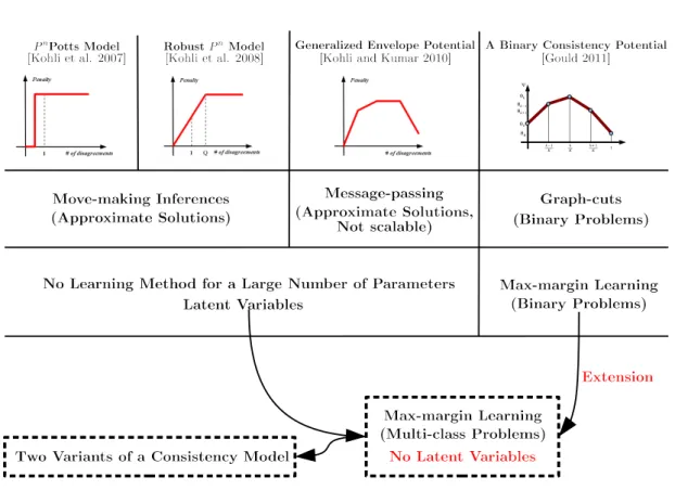
As a baseline model, a pairwise MRF model has been widely used in many com-puter vision problems. But recent higher-order models [Kohli and Kumar, 2010; Kohli et al., 2009, 2007; Ladicky et al., 2013; Ladick `y et al., 2012; Komodakis and Paragios, 2009] have demonstrated significant improvements over pairwise models

(20)

by incorporating constraints over large groups of nodes, i.e., cliques1. A successful example of higher-order models is the lower linear envelope model, which is also called a consistency model. The consistency model smoothes label assignments over cliques like pairwise models do over adjacent variables in pixel labeling problems. A simple consistency model is thePnPotts model [Kohli et al., 2007]. Later, the Robust

Pnmodel [Kohli et al., 2009] and the generalized model [Kohli and Kumar, 2010] with lower envelope functions were proposed, which allowed some inconsistent labels in cliques.

Figure 1.1 compares the multi-class pixel labeling tasks performed by a unary, a pairwise, and a higher-order model. As shown in Figure 1.1d, the label assignments by the unary model are too noisy and not coherent enough to recognize objects in the image. To improve the accuracy of the label assignment, the pairwise model employs additional constraints, e.g., the Potts model or contrast-sensitive terms to smooth out label assignments over adjacent variables. This model regularizes the assignment by the unary model by assuming that spatially close pixels tend to be in the same category. However, its capability to assign correct labels is limited as shown in Figure 1.1e due to its restricted connection to adjacent pixels. In Figure 1.1f, the higher-order model assigns labels consistently over cliques defined2 in Figure 1.1c, and the result is much better than that of the pairwise model. This higher-order consistency model utilizes low-level vision information such as color consistency and spatial closeness for clique definition.

In order to determine the best assignment for a given MRF problem, inference is performed via MAP estimation by minimizing the energy function of the MRF. Typically, exact MAP estimation is intractable for most graph structures. Only a few special structures of graphs are guaranteed to be solved exactly in polynomial time. Due to the limited inference solutions, the above multi-class pixel labeling prob-lems can be solved approximately, for example, by using move-making algorithms. Furthermore, higher-order models are required to develop their own inference algo-rithms since the structures are so diverse and complex that no standard solution for direct use is yet available. For instance, in Figure 1.1f, the image is represented by a densely connected graph containing a set of cliques. The subset of variables de-fined for the cow has an exponential number of possible assignments in the region.

1_{If the largest clique size is two, the model becomes a pairwise model. In the higher-order models}

(21)

grass tree cow sheep face body

(a) Image (b) True Labels (c) Superpixels (Cliques)

(d) Unary Model (e) Pairwise Model (f) Higher-Order Model

(22)

Thus, the joint distribution of variables over each clique is too large to estimate as a whole. One possible solution is to transform a higher-order model into a series of pairwise models by using additional auxiliary variables, but the computation time increases due to the increasing number of variables and the solution is approximate. Developing efficient inference algorithms for higher-order models is a difficult issue. Along with the demands for good model representations and efficient inference algorithms, an efficient training method is essential to maximize the performance of higher-order models. Model parameters are weighted to control the strength of individual terms in the model representation. By learning the parameters, we can generalize the model performance to novel examples. For pairwise models, sim-ple cross-validation has been generally used to find a small number of parameters, e.g., one or two parameters. However, as higher-order models involve a large number of parameters, the typical cross-validation approach is not a practical solution due to the increased search space. Instead, max-margin frameworks for the structured outputs [Tsochantaridis et al., 2006; Taskar et al., 2003; Joachims et al., 2009] can be considered an effective way of dealing with the large number of higher-order model parameters. In this learning, the energy function should be represented as a linear combination of the model parameters and the corresponding feature vectors that en-code each label assignment. In order to exploit this principled learning method, a higher-order model requires an encoding scheme to transform the energy function into a linear form. Another issue is that the max-margin learning problem can find suboptimal parameters [Finley and Joachims, 2008] if approximate inference algo-rithms are used in the framework, which is not limited to the learning problem of higher-order models.

The dual decomposition approach [Komodakis et al., 2011; Komodakis and Para-gios, 2009] was employed as an alternative inference method via a message-passing scheme for efficiently finding approximate solutions. In a similar way, Komodakis [2011a] showed that dual-decomposition can be applied to learning higher-order model parameters. The dual decomposition approach provides nice properties (such as convergence to a global optimum in the dual space and concurrent processing), but the higher-order models they used were too simple to be applied to generalized consistency models composed of multiple linear envelope functions.

(23)

et al., 2013] have not been completely investigated with a learning method for se-mantic scene segmentation. Kohli et al. [2009] proposed the Robust Pn model ex-tended from the previous model [Kohli et al., 2007] and derived efficient graph-cut based algorithms. But their approximate algorithms were restricted to the special form of consistency potentials (e.g., two linear functions per label). Then the robust model was generalized to the lower linear envelope potentials [Kohli and Kumar, 2010] composed of arbitrary number of linear functions. They showed how to apply a message-passing algorithm with multi-valued auxiliary variables, which provides approximate solutions. However, the models proposed above did not address the problem of learning the large number parameters except cross-validation. A hierar-chical consistency model [Ladicky et al., 2013, 2009] provided efficient move-making algorithms based on the RobustPnmodel, and also undertook experiments with real data sets. But they did not introduce a general training method such as the max-margin learning framework, rather they chose parameters based on greedy search-ing.

In this thesis, we search for and develop a unified framework for the consistency model. First, we employ a max-margin learning framework to treat an arbitrary number of parameters. Recently, Gould [2011] proposed a method for training a bi-nary consistency model using a max-margin learning framework. Inspired by Gould [2011], we propose a variant of the lower linear envelope model, which satisfies the linear constraint condition, to exploit the max-margin framework. Then, we extend this unified framework via a dual decomposition approach. In the dual decomposi-tion paradigm, we derive an efficient inference algorithm for the consistency model, expecting that it can find good model parameters by exactly minimizing surrogate functions encoded by the dual decomposition method. In the other part of this the-sis, we focus on improving the prediction performance of our model. We introduce a novel way of using global constraints to define cliques, and present regional features to customize general envelope potentials for each clique.

1 .

1 Contributions

(24)

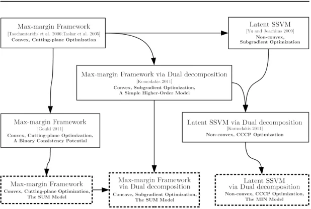
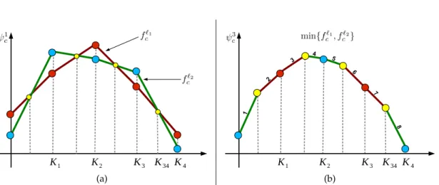
1. Generalized representation of the multi-class consistency model. We derive two different variants (i.e., ‘sum’ and ‘min’) of the consistency potential, which is the extension of the binary lower linear envelope function [Gould, 2011], to the multi-class case. Similar to Kohli and Kumar [2010], our model defines a concave penalty function over the number of variables taking a given label within a clique. This derivation generalizes the higher-order consistency terms with the lower linear envelope function in a compact form.

Considering the structured learning method, existing consistency models [Kohli and Kumar, 2010; Kohli et al., 2009] require iteratively estimating latent vari-ables in the model, which leads to a non-convex learning framework such as a latent structure SVM framework [Yu and Joachims, 2009]. However, using the ‘sum’ model, we can employ a standard max-margin framework, which is a convex problem, for our learning method.

2. Efficient MAP inference algorithms. The higher-order MRF models in

se-mantic pixel labeling problems have heavily connected nodes. Solving this multi-class MRF problem exactly is generally intractable. Thus, we propose ef-ficient approximate inference algorithms for our consistency models. We derive graph-cut based move-making algorithms using order-reduction techniques. Our algorithms can solve the energy function with general lower linear enve-lope functions, unlike Kohli et al. [2009] who showed how to perform approxi-mate move-making inferences with limited concave functions, but an arbitrary concave function can be decomposed as the sum of these limited functions. Compared to the message-passing algorithms proposed by Kohli and Kumar [2010], our move-making algorithms are generally faster according to the ex-periments performed by Kappes et al. [2013] and Szeliski et al. [2008].

(25)

3. Exploration of max-margin learning for the lower linear envelope model. Like most higher-order MRF models, the consistency model has a large number of parameters to learn because of multiple lower linear envelope functions. Thus, we require a principled learning framework to deal efficiently with an arbitrary number of parameters. We employ a structured learning paradigm, e.g., max-margin learning framework [Taskar et al., 2003, 2005; Tsochantaridis et al., 2006; Joachims et al., 2009]. Extending from Gould [2011], we show how to transform the energy functions into linear combinations of parameters and feature vectors, and derive additional linear constraints to maintain the concavity of our linear envelope functions.

We also exploit the max-margin framework via dual decomposition in which the dual surrogate losses are derived from the dual decomposition inference approach. We show that by minimizing the dual losses exactly through apply-ing our new minimization algorithm to the subproblems, this learnapply-ing method can find better model parameters than the previous primal learning method. In addition, because latent variables need to be estimated in the ‘min’ model, we cannot apply the standard max-margin framework. At this time, we provide latent max-margin learning via dual-decomposition [Komodakis, 2011b] with the ‘min’ model. Thus, we can accommodate our model within the standard learning frameworks.

4. Use of global constraints for clique definition. We use multiple

over-segmen-tations to define cliques for the consistency potentials in which pixels belonging to the same segment are grouped into a clique. Usually, Mean shift [Comaniciu and Meer, 2002] is used to decompose an image into locally coherent regions in terms of color and spatial distance. We introduce the Gaussian mixture model (GMM) as an alternative method for defining cliques over a large set of pixels. Importantly, these cliques do not need to be contiguous regions, but share com-mon features over disjointed regions as global constraints over the image. We show that GMM segmentation produces good cliques with clear object bound-aries and improves labeling accuracy in the model. Accordingly, we associate multiple higher-order terms with each segmentation, where the max-margin learning framework allows us to learn any number of parameters.

5. Using mid-level features for each clique. We propose an approach to

(26)

Figure1.2:Comparison of consistency models. Here we summarize the inference and learn-ing approaches of consistency models. The dotted boxes represent our contributions.

model depends very much on the quality of cliques, but not all cliques are defined over coherent regions. We define region features over cliques and mea-sure the quality of cliques. Then we use the feature responses for customizing general envelope functions for individual segmented regions. This additional mid-level feature increases the labeling accuracy significantly, but we reuse the previous inference and learning algorithms without modification.

Figure 1.2 and Figure 1.3 describe our contributions with the related works in terms of model representation and learning.

1 .

2 Thesis Outline

The remainder of this thesis is organized as follows:

Chapter2: Background. This chapter includes the related background theory needed

(27)

Figure1.3:Comparison of learning methods for structured outputs. This chart summaries a max-margin learning framework and its variants. The dotted boxes represent our contribu-tions to the problem of learning parameters.

major theoretical parts are based on various machine learning techniques, e.g., proba-bilistic graphical models, MAP inference algorithms, classification, and optimization. We also review relevant higher-order MRF models and superpixel generation.

Chapter 3: Higher-Order Consistency Models. We propose a generalized

repre-sentation of the consistency model. We also analyze the properties of the lower linear envelope functions, then show how to minimize the energy function of the proposed consistency model using efficient approximate move-making algorithms. Then we exploit a max-margin learning framework to learn the model parameters. In partic-ular, we present the key notion of encoding the lower linear envelope functions with a set of parameters and how to represent the energy function in a linearized form.

Chapter4: Multiple Higher-Order Consistency Models. We introduce a new use

(28)

Chapter 5: Learning via Dual Decomposition. We show how to integrate a dual

decomposition method into the MRF inference and the max-margin framework. Our new minimization algorithm to solve higher-order subproblems is proposed here. Also, we conduct experiments with real data sets and compare the results with pre-vious experiments.

Chapter 6: Using Region Features. We describe the idea of customizing general

linear envelope potentials for each clique. We define region features as ‘mid-level’ features and show how to modulate the envelope functions for individual cliques. After that, we evaluate the model with region features and compare the performance of all the models proposed in this thesis.

Chapter7: Conclusion. Last, we conclude with a summary of contributions, open

issues, and future directions.

1 .

3 Publications

The publications produced during this PhD course are:

1. Park, K.andGould, S., 2012. On learning higher-order consistency potentials for multi-class pixel labeling. InComputer Vision–ECCV 2012, 202–215. Springer 2. Park, K.; Shen, C.; Hao, Z.;and Kim, J., 2011. Efficiently learning a distance

metric for large margin nearest neighbor classification. InAAAI 2011.

(29)

Background and Related Work

Our work on a consistency model for multi-class pixel labeling problems is built on the foundation of a probabilistic graphical model [Koller and Friedman, 2009]. In this framework, we utilize compact representations, inferences, and learning meth-ods for our model. First, we explore the properties of probabilistic graphical mod-els. The graphical model describes the structure of a model in a compact form and provides an efficient joint reasoning process by combining local evidence and inter-dependence relationships. Then we explore some methods for Maximum a posteriori

(MAP) inference in graphical models. However, such MAP inference problems are generally NP-hard [Cooper, 1990; Koller and Friedman, 2009]. Thus, we make use of computationally efficient approaches for establishing approximate inferences.

Our graphical model is parameterized for each term, e.g., unary, pairwise, and higher-order terms, and the model is trained from a set of observed data in order to increase the prediction performance of the model given new instances of data. We ex-ploit various learning techniques for graphical models. Regression and classification algorithms provide pixelwise feature responses for unary potentials. A structured learning approach discovers optimal parameters needed to adjust each term of the graphical model.

The other part of this chapter introduces some examples of higher-order Markov random field (MRF) models and superpixel generation. Our model falls into a cate-gory of higher-order MRF problems and some existing higher-order models provide important notions and approaches for our model. Also, superpixels are an essential part of higher-order MRF models in computer vision. The segmented regions cre-ated by superpixel generation include groups of random variables which correspond with higher-order terms. We review the fundamental ideas of generating superpixels here.

(30)

2 .

1 Probabilistic Graphical Models

Probabilistic graphical models [Koller and Friedman, 2009] combine probability the-ory and graph thethe-ory to model joint probability distributions of structured random variables. In a graphical model, each node is associated with a random variable1

and an edge between nodes encodes the probabilistic interdependence between the corresponding variables. There are two different types of graphical representations: directed graphical models (also known as Bayesian networks) and undirected graph-ical models (also known as Markov random fields). All the graphgraph-ical models are useful to denote certain conditional dependencies between random variables. In this thesis, we focus on Markov random fields (MRFs), which satisfy local Markov prop-erties. The local Markov property requires that a random variable is conditionally independent of all other variables given its neighboring variables.

A benefit of graphical models is that they provide joint probability distributions in a compact form. Consider an undirected graph G with a set of random variables Y =_{Yi}ni=1. Then the joint probability distribution ofY is represented in a factorized

form as

Pr(Y) = 1

Z_c_∈C

∏

₍_G₎Fc(Yc), (2.1)

where C(_G) is a set of cliques2 in the graph G and Yc ⊆ Y is a subset of random

variables in a clique c. The functions Fc(Yc) are called factors and map the local

assignments to positive real values, which are not necessarily probabilities. The nor-malizing constantZ, also known as thepartition function, ensures that the sum of the probability distribution is 1. It is given by

Z=

∑

y∈Y

∏

c∈C(G)

Fc(Yc=y_c), (2.2)

where Y is the output domain ofY,y is a joint assignment toY, and y_c is the joint assignment toYc. The factor graph shows explicitly which random variables build

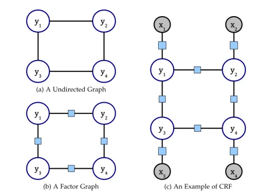
joint distributions. Examples of graphs are shown in Figure 2.1.

Conditional random fields (CRFs) [Lafferty et al., 2001] encode a conditional prob-ability distributionPr(Y _| X)of random variables Y and observed variables X. The CRFs also satisfy the local Markov properties conditioned on X. Thus, the

condi-1_{Because we associate a node with a random variable, we use the term ‘node’ to refer to the}

associ-ated random variable, or vice versa if there is no ambiguity.

(31)

(a) A Undirected Graph

(b) A Factor Graph (c) An Example of CRF

Figure2.1:Examples of Markov Random Fields and Factor Graphs. (a) is an example of an undirected graph and (b) is the factor graph of (a). The rectangles represent factor nodes. (c) is the factor graph specified by a conditional distribution, where the gray nodes are observed variables.

tional joint probability distribution is factorized with the observed conditionX = x as

Pr(Y = y_|X= x) = 1

Z(x)_c_∈C

∏

₍_G₎Fc(yc;x), (2.3)

where y_c is an assignment to the corresponding variables in cliquec. Note that the factors Fc(yc;x) are conditioned on x. Also, the main difference between MRF and

CRF is that in CRFs, the normalization constantZ(x)becomes a function ofX as

Z(x) =

∑

y∈Y

∏

c∈C(G)

Fc(yc;x). (2.4)

(32)

2.1.1 Energy Function

In Equation (2.1), the factorsFc(yc), which are positive, can be transformed into the

logarithmic representation as

ψc(yc) =−logFc(yc), (2.5)

where we refer toψc(yc)as the potential functionor clique potentialon clique c. Then

the joint distribution of Y can lead to an alternative representation of the energy function E(Y =y)as

Pr(Y =y) = 1

Zexp −_c

∑

_∈Cψc(yc)

!

(2.6)

= 1

Zexp

−E(Y =y). (2.7)

The energy function provides a compact representation for many distributions; in-stead of encoding factors with a complete set of values of variables, clique potentials can have sparse representations capturing certain patterns of values of variables, e.g., 1 when two variables take the same value and 0 otherwise. Furthermore, the sum of potential functions makes it easy to be parameterized with a family of distri-butions associated with feature functions (e.g., factors). Significantly, the main bene-fit of the transformation into log-space is to avoid numerical issues with multiplying many small probabilities.

To be concise, we denote the probability ofY =yasPr(y)and the energy function of Y = y as E(y), and use the terms MRF and CRF interchangeably if there is no ambiguity.

2.1.2 MAP Inference and Energy Minimization

Since the logarithmic transformation of Equation (2.7) leads to an inverse propor-tional relationship between the log probability distribution and the energy function as

logPr(y)∝₋_E(y), (2.8)

aMaximum a posteriori(MAP) inference is equivalent to the energy minimization:

argmax y∈Y

Pr(y) =argmin y∈Y

(33)

An advantage of MAP inference is that it does not require computation of the normal-ization constant Z, which is summed over all possible joint assignments. However, MAP inference is still computationally intractable for general graphs [Cooper, 1990; Koller and Friedman, 2009]. Only a few special cases are known for exact inference. For example,

• For a chain- or tree-structured graph, message-passing algorithms can yield exact solutions [Barber, 2012; Pearl, 1988, 1982].

• For binary pairwise MRF/CRF models with sub-modular energy functions, there exist graph-cut based algorithms for exact inference [Kolmogorov and Zabih, 2004].

If exact inference is not available, we need to use approximate inference algorithms such as loopy belief propagation [Yedidia et al., 2005; Weiss and Freeman, 2001], move-making algorithms [Kolmogorov and Zabih, 2004; Boykov et al., 2001; Besag, 1986], or linear programming relaxation [Wainwright and Jordan, 2008; Werner, 2007; Schlesinger, 1976].

2.1.3 Min-Cut / Max-Flow

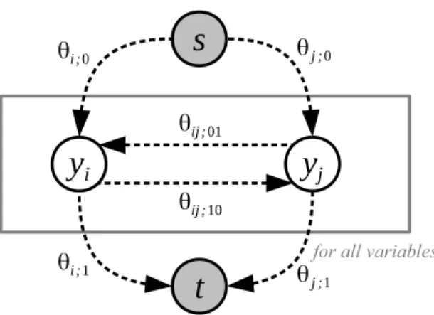
Graph-cuts are a family of algorithms to efficiently minimize a certain type of energy function (e.g., a binary pairwise submodular function) exactly in polynomial time regardless of the structure of the graphs. The basic idea of the algorithm is to trans-form the energy function into a special graph that contains two auxiliary terminal nodes, i.e., the sources and the sinkt, and a non-negative weight for each edge. By minimizing the cost to cut thisst-graph, we obtain an optimal solution which mini-mizes the original energy function [Kolmogorov and Zabih, 2004]. After cutting the graph, the nodes are separated into two groups which belong to each terminal node. This min-cut problem is also known to be equivalent to the maximum flow problem by the theorem of Ford and Fulkerson [1962].

As stated above, the special case of the energy function – a binary pairwise sub-modular function – can be solved exactly using graph-cuts. To encode the special energy function, we define a quadratic pseudo-Boolean function (QPBF), which is convenient for mapping to anst-graph directly.

(34)

andR_{a real domain. A mapping}

f :Bn_→R _(2.10)

is then called apseudo-Boolean function[Boros and Hammer, 2002].

A quadratic pseudo-Boolean function is a polynomial of degree 2 and can be written as

f(y) =c0+

n

∑

i=1

ciyi+

∑

i<_j

cijyiyj , (2.11)

with variables yi ∈ B and coefficients ci and cij. A pairwise binary MRF is

equiva-lently represented as a quadratic pseudo-Boolean function (QPBF) [Boros and Ham-mer, 2002]. Here we write the QPBF inposiformas

f(y) =θconst+

∑

i

θi;0yi+θi;1yi

+

∑

(i,j)

θij;00yiyj+θij;01yiyj+θij;10yiyj+θij;11yiyj , (2.12)

wherey_i =1−yi and all coefficientsθa;bare non-negative with the possible exception

of the constant term θconst. Note that this posiform parameterization is not unique.

For example, we can add an arbitrary non-negative constant to bothθi;0 andθi;1 and

subtract it fromθconst without changing the energy of any assignment.

A quadratic pseudo-Boolean function is calledsubmodular if each set of pairwise coefficients{θij;ab |a,b∈B}satisfies

θij;00+θij;11 ≤θij;01+θij;10 (2.13)

[Boros and Hammer, 2002], or equivalently in (2.11),

cij ≤0 (2.14)

for all pairwise coefficients [Nemhauser et al., 1978]. With respect to pixel label-ing problems, for instance, both Potts prior and the contrast-sensitive prior satisfy submodularity3, which implies that θij;00 = θij;11 = 0 and θij;01 = θij;10 > 0 for all

variable pairs (i,j). Figure 2.2 illustrates the st-graph constructed from (2.12) with 3_{Potts prior}_θ

(35)

Figure2.2: Example of an st-graph of a pairwise binary submodular energy function with

θij;00 = θij;11 = 0. Given a graph G, we add two auxiliary nodes, the source node s, and

the sink node t to the graph. Once all edges of the resulting graph are assigned by clique potentials of the original problem, computing max-flow gives an equivalent solution to min-imizing the original problem. The maximum flow (capacity) of anst-graph is known to be a graph-cut for a minimum path from the nodesto the nodet.

θij;00 =θij;11 =0. Given anst-graph, there exist many algorithms to solve the problem

such as augmented paths [Ford and Fulkerson, 1962] and push-relabel algorithms [Goldberg and Tarjan, 1988].

The goal of inference is to find the assignmenty⋆

with minimum energy. Message-passing algorithms can be suitable for the purpose, but it is well known that for submodular pairwise energy functions, this can be done efficiently by finding the minimum-cut in a suitably constructed graph [Szeliski et al., 2008; Boykov et al., 2001; Kolmogorov and Zabih, 2004]. Unfortunately, in general, for multi-label CRFs (or indeed, non-submodular binary CRFs), inference is intractable and we need to resort to approximate routines.

2.1.4 Move-making Inference

(36)

assign-ments y_t _{∈ {}yprev_{} ∪ Y}t, whereYt _{is a subset of candidate assignments at the} _t_-th

iteration and in general Yt _{⊂ L}n_{. If the algorithm finds a lower energy} _E₍_y

t)than

the previous energyE(yprev), the assignmenty_tis updated asynext. Otherwise,yprev is kept asynext.

An early example of move-making algorithms is Iterated Conditional Modes (ICM) [Besag, 1986]. For a given variable, it finds the optimal assignment condi-tioned on all the other variables. However, the update of a single variable makes its convergence slow and can easily get stuck in poor local optima. More advanced examples of move-making algorithms are α-expansion and αβ-swap [Boykov et al., 2001; Kolmogorov and Zabih, 2004]. They use graph-cuts for finding the optimal move in which each move restricts the label space of variables to at most two values from the label set and the resulting binary energy function must be submodular. In

α-expansion, each label α is chosen from L iteratively. Then each variable switches to the chosen label α or keeps the current assignment, which expands the current labelαto other variables. It continues to iterate through the label set until the energy reduces no more. Similarly, duringαβ-swap, a pair of labelsαand βis chosen from

L iteratively. Then it makes moves by swapping only between the variables with either of the two labels and holds fixed all the other variables which do not take the label αor β. In summary, the three algorithms are characterized as follows:

• ICM: for a given variable i, we choose theynext

i ∈ L that minimizes the energy

withynext

j =y

i ∈ {y

energy.

• αβ-swap: for all i such that yprev_i ∈ {α,β}, we choose the ynext_i ∈ {α,β} that jointly minimize the energy andynext_j =yprev_j for all other variables (j6=i). Forα-expansion andαβ-swap, an efficient graph-cut based implementation has been proposed to minimize the energy functions found in computer vision [Boykov and Kolmogorov, 2004].

2.1.5 Higher-Order MRF Models

(37)

shown superior performance to pairwise models (e.g., in semantic image segmenta-tion [Ladicky et al., 2013, 2009]). Given a graphG =_{V,E,C}composed of nodesV, edgesE, and cliquesC, a higher-order energy function is generally represented with potential functionsψ=_{ψi,ψij,ψc}respectively as follows:

E(y) =

∑

i∈V

ψi(yi)

| {z }

Unary Terms +

∑

(i,j)∈E

ψij(yi,yj)

| {z }

Pairwise Terms

+

∑

c∈C

ψc(y_c)

| {z }

Higher-Order Terms

, (2.15)

where the cliques can be defined on subsets of nodes, or even all nodes to encode global constraints. As the large number of variables are jointly estimated over the cliques, efficient inference algorithms are demanded for solving the higher-order models. One popular method is to reduce a higher-order energy function to a group of pairwise potentials and use the existing inference algorithms such as graph-cuts [Kohli et al., 2009, 2007; Ladicky et al., 2013; Delong et al., 2012]. Such methods are able to solve the problems efficiently; however, they are limited to a specific range of problems, e.g., submodular energy functions. Other attempts include dual ap-proaches [Komodakis et al., 2011; Wang et al., 2010; Werner, 2008, 2010] and belief propagation based methods [Lan et al., 2006; Tarlow et al., 2010] which extend pair-wise cases to higher-order models.

Here, we review some important examples of existing higher-order models, which are relevant to the work presented in this thesis.

2.1.5.1 Extended PnModels

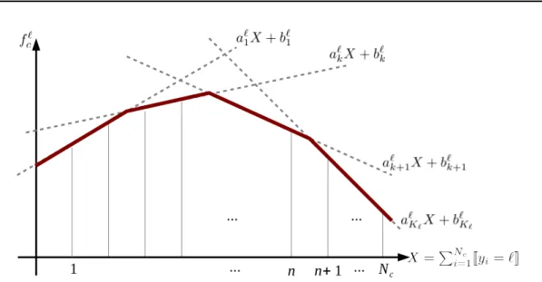
The Pn _{Potts model [Kohli et al., 2007] and its successors encourage all variables}

belonging to a clique to take the same label. These models encode a penalty, with the number of variables taking a given label, and hence they smooth the annotations within cliques, which is similar to pairwise smoothness prior between neighboring variables. The Pn_{Potts model is defined as}

ψc(y_c) =

  

γℓ ify_i = ℓ, ∀i∈c

γmax ifyi = ℓ′(6=ℓ)∃i∈c

, (2.16)

where γmax ≥ γℓ,∀ℓ ∈ L. This model rigidly enforces consistent label assignments

over each clique. For example, the same maximum penalty γmaxis imposed unless

(38)

(a)PnModel (b) RobustPnModel (c) Lower Envelope Model

Figure2.3:Three examples of consistency models. These potentials take the number of vari-ables for a given label and penalize the number of inconsistent assignments over a clique. (a) prefers complete agreement within variables. (b) has some robustness for some inconsistency. (c) generalizes the robustness with a piecewise lower linear envelope function.

et al., 2009] defines a linear truncated function of the number of inconsistent variables as

ψc(y_c) =min

min

ℓ_∈L (|c| −Xℓ)θℓ+γℓ,γmax

, (2.17)

where Xℓ is the number of variables which take a labelℓ in clique cand θℓ is a

po-tential function parameter. Unlike the Pn _{Potts model, the Robust}_Pn_{model reduces}

the penalty if only a small number of variables in a clique take different labels. Later, this model was generalized as the lower linear envelope model composed of multiple linear functions [Kohli and Kumar, 2010]. Three models are illustrated in Figure 2.3. Note that Kohli and Kumar [2010] also proposed the lower linear envelope model as well as the upper linear envelope model. This type of higher-order potential for-mulates size prior and not-null set constraints, which, for instance, enforce a fixed number of scene elements such as pixels or regions to be assigned a particular label. However, this involves a difficult min-max optimization problem and is not consid-ered in this thesis.

2.1.5.2 Other Models as Global Constraints

A Label Co-occurrence Model. The co-occurrence model [Ladick `y et al., 2012]

(39)

subsets of highly correlated object classes. They showed how energy functions incor-porated with such global constraints could be minimized in various ways (e.g., lin-ear program relaxation, using message-passing algorithms, and move-making algo-rithms).

A Label Cost Model. Another global potential appears in the label cost model

[De-long et al., 2012]. Their model is concerned with the number of labels or subsets of labels in an image and forces certain subsets of labels to be present. This work has demonstrated some applications – such as unsupervised image segmentation and motion segmentation where the number of segmentations is unknown – and has employed graph-cut based formulations. This potential function can be constructed with the (robust) Pn Potts model by encoding a penalty over all variables taking a specific subset of labels.

2 .

2 Superpixels and Regions

A superpixel is an over-segmented image patch in which the pixels are grouped with respect to similar features. Superpixels have been employed in many computer vision problems since Ren and Malik [2003] proposed it for reducing computational complexity. They represented a large set of pixels as a single superpixel, reducing the number of random variables to a single random variable.

In our consistency model, superpixels are used to define cliques for higher-order terms rather than for efficiency. Therefore, our approach is more flexible than adding the hard constraint that all pixels in a superpixel be labeled the same. Here, we review the superpixel algorithms used in our work as well as other vision problems.

2.2.1 Mean Shift

Mean shift [Comaniciu and Meer, 2002] is a non-parametric clustering method which considers feature space as a probability density distribution. Given a set of data points, the main idea is to find a higher density location of them by assuming that they are sampled by a probability density function (pdf). After iteratively updating the mean shift vector, all points that have converged to the same stationary point are considered as belonging to the same cluster.

(40)

the size of windows for kernel function estimation. Here the kernel functions (or pdfs), generally refer to uniform, Gaussian, and Epanechnikov distributions.

Assume each of n data points xi ∈ Rd has a probability density function K(·).

The multivariate kernel density estimate f(_·)is written as

f(x) = 1

nhd n

∑

i=1

K

x₋xi h

, (2.18)

where the kernel functionK(_·)has a window size h(called a radius of the kernel or bandwidth). By taking gradient steps of the function f(_·), we can compute the mean shift vectorm(x)

m(x) = ∑

n

i=1xig x−_hxi

∑n_i=₁g x−xi

h

−x, (2.19)

where g(x) = ₋K′(x). In short, the mean-shift procedure can be summarized as follows: For each point xi

1. Compute mean shift vectorm(xt)for thet-th iteration. 2. Update the density estimation center, i.e.,xt+1= xt+m(xt). 3. Repeat until all points have converged.

4. Then group all points which have the same convergence point.

For superpixel generation, (Luv) color and spatial distances are used for the band-width. Other applications using mean shift include discontinuity preserving smooth-ing applications and tracksmooth-ing [Comaniciu et al., 2003].

2.2.2 Gaussian Mixture Models

A Gaussian mixture model (GMM) is defined by the sum of multiple weighted prob-ability density functions, in particular a strong assumption as to a Gaussian distribu-tion

N(x _|µ,Σ) = 1 (2π)d2p|Σ|

exp

−1₂(x₋µ)⊤Σ−1(x₋µ)

, (2.20)

wheredis the dimension ofxand(µ,Σ)is a pair of parameters such as the mean and the covariance matrix of the Gaussian. Given a set of data X = _{x_} sampled from an unknown distribution, we model the unknown distribution with mixture of K

(41)

and the mixture components that the data belong to. The probability density function of the GMM is defined as

p(x) =

K

∑

k=1

ωkN(x |µk,Σk) (2.21)

s.t.

K

∑

k=1

ωk= 1 (2.22)

0≤ωk≤1 , (2.23)

whereωkis the prior probability (weight) of thek-th Gaussian. If the model

parame-ters are known, it is easy to estimate which distribution each data point belongs to or vice versa. However, the main objective is to find out the label belonging to each data point and to approximate the model parameters at the same time. In this case, the EM algorithm [Dempster et al., 1977; McLachlan and Krishnan, 2007] is used to opti-mize the above problem. The ‘E’ step estimates the probability of each Gaussian for each data point and the ‘M’ step updates the parameters to maximize the likelihood of the data. After training this model, we can produce superpixels by evaluating the dataxp of each pixel pas

k⋆ =argmin

k

N(xp|µk,Σk), (2.24)

where k⋆ is the cluster to which the pixel pbelongs. However, this model has some issues. First, it is very sensitive to initialization. Second, the user has to set up the number of Gaussians.

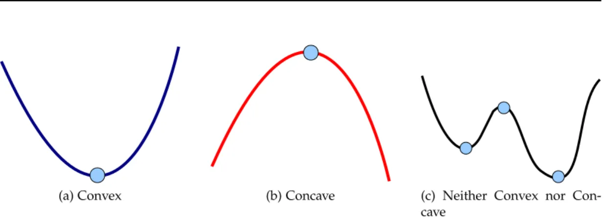
2.2.3 Other Clustering Algorithms

(42)

(a) Convex (b) Concave (c) Neither Convex nor Con-cave

Figure 2.4: Three examples of general functions: convex, concave, and neither. The circle represents saddle points (of either global or local optima).

2 .

3 Convex Optimization and the Dual Problem

Many computer vision problems involve various multi-dimensional functions and constraints. The aim of the optimization of a multi-dimensional function is to find a saddle point of the function subject to constraints. That is, let a function f be defined as a mapping ofx_{∈ X} to the real domain, i.e.,

f :X →R_, _(2.25)

where_X is a subset of the real spaceRn_{. Then the minimization of the function} _f_,

minimize

x∈X f(x) (2.26)

finds a point x⋆ _{∈ X} such that

f(x⋆)_≤ f(x) _∀x_{∈ X} . (2.27)

Here, the function f is called an objective function or a cost function. In general, the domainX is bounded by some conditions known as constraints.

Depending on the shape of the function f, we may get one or multiple saddle points. In (2.27), f(x⋆)is called a global minimum if the function f(_·)is convex on the domain X. In Figure 2.4, each of the convex and the concave function have a global optimum point. However, convex functions can have more than one global minimum point.

(43)

defined as a convex optimization problem [Boyd and Vandenberghe, 2004] as follows.

Definition 2.3.1. A constrained minimization problem

minimize

x f0(x) (2.28)

subject to fi(x)≤0 ∀i hj(x) =0 ∀j

is a convex optimization problem if the objective function f0and the inequality constraints fi are convex, and the equality constraints hj are affine.

Similarly, a concave maximization problem is another form of convex optimiza-tion problem when the negative objective funcoptimiza-tion−f0is maximized.

2.3.1 Dual Problem

Consider the problem (2.28), which is called aprimal problem. The Lagrangian func-tion of Equafunc-tion (2.28) is

L(x,λ,µ) = f0(x) +

∑

i

λifi(x) +

∑

j

µjhj(x), (2.29)

where we associate Lagrangian multipliersλi ≥0 andµj with constraint functions fi

andhj. We call the Lagrangian multipliers the dual variables associated with (2.28).

Using the Lagrangian function (2.29), we define the Lagrangian dual of the primal problem as the minimum value of (2.29) over x:

LD(λ,µ) =inf

x L(x,λ,µ). (2.30)

This dual becomes −∞ _{when the Lagrangian (2.29) is unbounded below in} x. Note that the Lagrangian dual is a concave function ofλ andµ because the dual function is a pointwise infimum of affine functions ofλ andµ. Thus, this leads to a concave problem. Even though the primal is not convex, the dual function is still concave, which is why the dual is preferred.

(44)

problemis presented to find the optimal lower bound as follows:

maximize

λ,µ LD(λ,µ) (2.31)

subject to λi ≥0 ∀i.

Let d⋆ be the optimal value of the dual problem at(λ⋆,µ⋆) and p⋆ be a counter value of the primal problem at x⋆. The difference between the two values p⋆−d⋆

is called the optimal duality gap. If the inequality d⋆ ≤ p⋆ holds, it is called a weak duality. If the gap is zero, we call it a strong duality. In particular, if we know a dual optimal solution (λ⋆,µ⋆) and a strong duality holds, we can sometimes interpret the primal solution x⋆ in terms of the dual solution. For more detail on convex optimization, refer to Boyd and Vandenberghe [2004]

2 .

4 Learning Model Parameters

Our work exploits various machine learning algorithms. Here, we are concerned with supervised learning in which a set of training data is used to adjust model parameters and to lead the model to determine the best outputs for a set of novel data. The outputs can be discrete values, continuous values, or structured outputs. In this section, we provide an overview of learning algorithms related to our model.

2.4.1 Regression and Classification

Regression is a statistical process to predict a target valuey∈R_{which is continuous.}

Specifically, a function fof unknown parametersθand an observed valuexestimates the corresponding true valuey, i.e.,

f(x;θ)_≈y. (2.32)

One simple regression model,linear regressionassumes the target variableycan be ap-proximated by a linear combination of values and parameters, i.e., f(x;θ) =θ⊤x+η, where η is unknown random noise (typically assumed to be a zero-mean Gaussian distribution). Using a set of training data {(xi,yi)}i=N1, we can estimate the

(45)

Figure2.5:Example of logistic regression. The logistic (or sigmoid) function measures prob-abilities of data points which range from−∞_to∞_{. The circles and squares are two different} types of data, labeled 0 and 1.

values and predicted values) as

minimize

θ

N

∑

i=1

kyi− f(xi;θ)k22 . (2.33)

To prevent the model being overfitted, the ℓ₂_-regularizer _k_θ_k2

2 is added to the cost

function (2.33), which maintains the convexity of the problem. While the ℓ₂ _norm

can provide numerical stability and prevent overfitting, the ℓ₁ _{norm can provide}

robustness to outliers having sparse parameters.

2.4.1.1 Logistic Regression Models

Logistic regression is a classification method rather than a regression, which uses a probabilistic interpretation. This method introduces a non-linear mapping where the linear regression cannot fit to a data set. To understand logistic regression, let us review a binary classification problem first, and a multi-class classification problem next. Logistic regression (LR) uses a logistic functionσ(z)

σ(z) = 1

1+e−z (2.34)

in order to consider a probabilitypof datax. As shown in Figure 2.5,zgoes from−∞

(46)

logit is written as

z=log(odds) = ln( p

1−p) (2.35)

=θ⊤x+b, (2.36)

where p is the probability of the case ‘1’. By using the notion of odds, we can con-vert non-linear mapping to linear mapping, which makes the optimization possible as in linear regression. We get the σ(z) as the posterior probability that y = 1, i.e., Pr(y=1|x) =σ(z). For classification, we interpret σ(z) > _{0.5 as} _y ₌ _{1, and}

otherwise asy =0.

For learning the parameters(θ,b), we compute the maximum likelihood of target valuesYgiven observed values X

Pr(Y _|X) =

N

∏

i=1

1

1+e−yiz(xi) (2.37)

assuming thatN training examples are independent. Then a loss function is defined by the negative log likelihood. With a convex regularizerkθ_k2_{, the learning problem}

is given as

minimize

θ

N

∑

i=1

log(1+e−yiz(xi)_{) +}_λ_k_θ_k2

2 , (2.38)

whereλis the regularization constant.

Multi-class logistic regression, also called softmax regression, is the extension of the binary model to discriminate a set of more than two classes. Instead of taking one linear parameter vector, we combine multiple linear parameters with a feature vector for multi-class cases. For a class ℓ _{and a feature vector} _x_{, a logit function} z(ℓ_,_x_;_θ_{) =}_θ⊤_ℓ_x _{is defined, where} _θℓ is the parameter vector for classℓ. After

com-puting all the regression values by using a set of binary regressions, we normalize the probability of each class. Thus, the probability of classℓ_{is defined as}

Pr(y=ℓ_|_x_;_θ_{) =} exp(θ ⊤

ℓx)

∑L_i=₁exp(θ⊤_i x) , (2.39)

where L is the number of classes. This multi-class LR discriminates the most likely assignment which gives the maximum probability, e.g.,y⋆

(47)

a regularization term, i.e.,

minimize

θ

N

∑

i=1

−logPr(yi |xi;θ)

+λkθ_k2₂, (2.40)

whereλis the regularization constant.

In CRF models, we use this multi-class logistic regression as unary potentials to score local features.

2.4.1.2 Boosting Algorithms

Boosting [Schapire, 1990, 2003; Meir and Rätsch, 2003] is an additive classification method. The main idea is to build a strong classifier by combining weak classifiers. Here a weak classifier means any classifier with accuracy better than a random guess (e.g., the accuracy is higher than 0.5 in binary classification problems). There are many variations of boosting such as AdaBoost [Freund and Schapire, 1997], LPBoost [Demiriz et al., 2002], TotalBoost [Warmuth et al., 2006], BrownBoost [Freund, 2001], MadaBoost [Domingo and Watanabe, 2000], LogitBoost [Friedman et al., 2000], and AnyBoost [Mason et al., 2000].

We will assume a binary classification problem in this section. A decision func-tion H(x) is constructed out of a linear combination of weighted weak classifiers

ht(x):Rn→ {−1, 1}:

H(x) =sign

T