White Rose Research Online URL for this paper:
http://eprints.whiterose.ac.uk/149113/
Version: Accepted Version
Proceedings Paper:
Conserva Filho, M. S., Marinho, R., Mota, A. et al. (1 more author) (2018) Analysing
RoboChart with probabilities. In: Massoni, Tiago and Mousavi, Mohammad Reza, (eds.)
Formal Methods:Foundations and Applications - 21st Brazilian Symposium, SBMF 2018,
Proceedings. 21st Brazilian Symposium on Formal Methods, SBMF 2018, 26-30 Nov 2018
Lecture Notes in Computer Science (including subseries Lecture Notes in Artificial
Intelligence and Lecture Notes in Bioinformatics) . Springer Verlag , pp. 198-214.
https://doi.org/10.1007/978-3-030-03044-5_13
[email protected] https://eprints.whiterose.ac.uk/
Reuse
Items deposited in White Rose Research Online are protected by copyright, with all rights reserved unless indicated otherwise. They may be downloaded and/or printed for private study, or other acts as permitted by national copyright laws. The publisher or other rights holders may allow further reproduction and re-use of the full text version. This is indicated by the licence information on the White Rose Research Online record for the item.
Takedown
If you consider content in White Rose Research Online to be in breach of UK law, please notify us by
M. S. Conserva Filho1, R. Marinho1, A. Mota1, and J. Woodcock2
1
Centro de Inform´atica, Universidade Federal de Pernambuco, Brazil
{mscf,rma6,acm}@cin.ufpe.br 2
Department of Computer Science, University of York, UK
Abstract. Robotic systems have applications in many real-life scenar-ios, ranging from household cleaning to critical operations. RoboChart is a graphical language for describing robotic controllers designed specif-ically for autonomous and mobile robots, providing architectural con-structs to identify the requirements for a robotic platform. It also pro-vides a formal semantics in CSP. RoboChart has a probabilistic operator (P) but no associated probabilistic CSP semantics. When P is used, currently a non-deterministic choice (⊓) is used as semantics; this is a conservative semantics but it does not allow the analysis of stochastic properties. In this paper we define the semantics of the operatorP in terms of the probabilistic CSP operator⊞. We also show how this aug-mented CSP semantics for RoboChart can be translated into the PRISM probabilistic language to be able to check stochastic properties.
Keywords: Robotic systems, CSP, probabilistic analysis, PRISM
1
Introduction
Robotic systems have been used in many real-life scenarios, ranging from simple domestic assistants [18] (household cleaning) to safety-critical activities, such as driverless cars [4] and pilotless aircraft [27]. Despite their complexity, the current practice for implementing such robots applications is performed in an ad-hoc manner. These practices are often based on standard state machines, without formal semantics, to describe the robot controller only.
In [21], a domain-specific modelling language, called RoboChart, based on UML, is proposed. It is a graphical language for describing robotic controllers, specifically designed for autonomous and mobile robots. It provides architectural constructs to identify the requirements for a robotic platform. Features of the RoboChart graphical notation allow, for instance, the behavioural description of timed, continuous, and probabilistic properties.
Concerning formal verification, RoboChart has a formal semantics in CSP [23] that can be automatically calculated by RoboTool3, a tool that supports the use of RoboChart. CSP is a well established process algebra to model and verify con-current systems. It defines the behaviours of a system in terms of events and the
3
interactions of processes. CSP has support for model checking with FDR [25], which provides a high degree of automation for early validation. Using FDR, we can, for instance, establish determinism, and absence of deadlock and divergence. Besides functional aspects, RoboChart has also a probabilistic operator (P) that can be used to express stochastic behaviours. Currently, however, it has no associated probabilistic CSP semantics. When it is present, for instance, between processesP andQ, a non-deterministic choice (P ⊓Q) is used as semantics.
The work reported in [8] presents a version of FDR supporting the probabilis-tic operator ⊞. But instead of modifying the FDR algorithm itself to perform probabilistic analysis, the work [8] adds a new algorithm that creates a PRISM specification [14] from a probabilistic CSP specification. This translation was namedWatchDog Transformation. PRISM is a probabilistic language and model checking tool (both have the same name) which has already been successfully de-ployed in a wide range of application domains, such as real-time communication protocols, robots applications, and biological signalling pathways.
In this paper we define the semantics of the RoboChart probabilistic operator P in terms of the CSP probabilistic operator ⊞, preserving all the original CSP semantics of RoboChart. To check for probabilistic properties, we specify a CSP property specification; this is different from the usual way of handling probabilistic model checking, which is based on a temporal logic language to express properties. We then reuse theWatchDog Transformationprovided by [8], which combines the two CSP processes (property and process under analysis), yielding a PRISM specification. With this specification, we just have to check for a specific probabilistic temporal logic formula using the PRISM tool.
The remaining of this paper is structured as follows. The next section provides an overview of RoboChart, and its CSP semantics. Section 3 briefly presents PRISM. The translation from CSP to PRISM is discussed in Section 4. Section 5 presents our proposed strategy, and case studies are described in Section 6. Finally, we draw our conclusions, and discuss future work in Section 7.
2
RoboChart
RoboChart [21] is a UML-like notation designed for modelling autonomous and mobile robots. It provides constructs for capturing the architectural patterns of typical timed and reactive robotic systems, and probabilistic primitives as well. As opposed to other approaches for describing robotic systems, RoboChart has a formal semantics that can be automatically calculated.
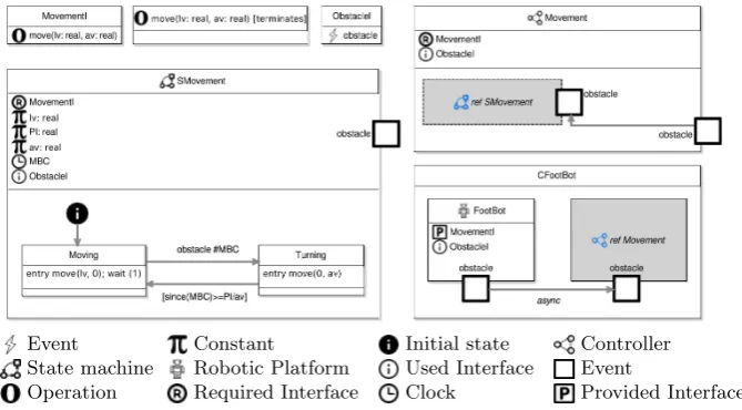
We give an overview of RoboChart using a toy model, as illustrated in Fig-ure 1. A robotic system is defined in RoboChart by a module. In our example, it is calledCFootBot, and specifies a robot that can move around and detect obsta-cles. A module contains a robotic platform and one or more controllers that run on this platform. The robotic platformFootBotdefines the interface of the sys-tem with its environment, via variables, operations, and events. In our example, the operationmove(lv,av)captures the movement of the robot with linear speed
to any object in its environment; it is an abstraction of a sensor that detects obstacles. There may be one or more controllers, interacting with the platform via asynchronous events, and between them via synchronous or asynchronous events. Our example has just a single controllerMovement. The behaviour of a controller is defined by one or more state machines, specifying threads of execu-tion. Here, the behaviour of Movementis defined by the machineSMovement.
Event Constant Initial state Controller
State machine Robotic Platform Used Interface Event
[image:4.595.136.471.213.398.2]Operation Required Interface Clock Provided Interface
Fig. 1.RoboChart: obstacle detection
Interfaces can group variables, operations, and events. In Figure 1, the in-terfaceMovementI has only the operation move(lv,av), provided by the robotic platform, and required by the controller. ObstacleI has just the eventobstacle, which is used in the platform, the controller, and the state machine. In general, different events may be connected, as long as they have the same type, or no type. Types are used when an event communicates an input or output value.
A state machine is the main behavioural construct of RoboChart. It is similar to that in UML, except that they have a well defined action language. In our example, the behaviour of SMovement is as follows: upon entry in the state
Moving, after calling the operationmove(lv,0), the robotwaits for one time unit. The operation callmove(lv,0)takes no time; it can be, for example, implemented as a simple assignment to the register of an actuator. The machine, however, is blocked bywait(1)for one time unit (which is a budget for the platform to react to this operation) before it completes entry toMoving.
SMovementdeclares a clockMBC. In Moving, when an obstacleis detected,
MBC is reset (#MBC) and the machine moves to the state Turning. There, a call move(0,av) turns the robot. A transition back to Moving is guarded by
PI/av, to ensure that the robot waits enough time to turn PI degrees, before going back toMoving, and proceeding in a straight line again.
There may be one or more controllers, interacting with the platform via asynchronous events, and between them via synchronous or asynchronous events. Here, we have just a single controllerCForaging. The behaviour of a controller is defined by one or more state machines, specifying threads of execution. In the example, the behaviour of CForaging is defined by the machineSForaging.
Interfaces can group variables, operations, and events. In Figure 1, the inter-faceIForaginghas the eventsstop,forageandflip, which are used in the platform, the controller, and the state machine. In general, different events may be con-nected, as long as they have the same type, or no type. Types are used when an event communicates an input or output value.
Further information regarding RoboChart can be found in [21, 22, 20].
2.1 Semantics
The semantics of RoboChart is defined using a dialect of CSP called tock-CSP [23]. It is used to describe concurrent reactive systems that are composed by interacting components, which are independent entities called processes, that can be combined using high level operators to create complex concurrent sys-tems. In tock-CSP, a special event tock marks the discrete passage of time.
Before presenting the semantics for our example, we first introduce the re-quired CSP syntax. The processSKIP represents the terminating process, and
STOP represents a deadlock process. The prefixing a → P is initially able to perform only the simple eventa, and behaves like process P after that. Events may also be compound. For instance,b.n is composed by the channelband the value n. The process P 2 Q is an external choice between process P and Q. The process P; Q combines the processes P and Q in sequence. The process
if b then P else Q behaves asP ifb holds and asQ otherwise. Further informa-tion regarding CSP can be found in [23].
We present below a CSP process CFootBot that specifies the behaviour of our example in Figure 1. The formal semantics of RoboChart is implemented by a tool (RoboTool) that automatically calculates a process that is equivalent to
CFootBotbelow.
CFootBot=EMoving; Obstacle; ETurning; wait(PI/av); CFootBot
CFootBotcomposes in sequence processesEMoving,Obstacle,ETurning, and
wait(PI/av)followed by a recursive call.EMovingis below; it engages in the event
moveCall.lv.0, which represents the operation callmove(lv,0)in the entry action of the stateMoving. In sequence (prefixing operator→),EMovingengages in the
moveRet event that marks the return of that operation, and then behaves like the processwait(1).
EMoving=moveCall.lv.0→moveRet→wait(1)
The definition of the parameterised processwait(n) is recursive; it engages in n occurrences of tock to mark the passage of n time units, and after that terminates: SKIP. So, wait(1) corresponds directly to the wait(1) primitive of RoboChart. The process Obstacle defined below allows time to pass until an eventobstacle occurs, when it then terminates. So, the eventsobstacle andtock
are offered in an external choice (2).
Obstacle=obstacle→SKIP 2tock →Obstacle
Finally, the processEntryTurning models theentryaction of Turning.
EntryTurning=moveCall.0.av→moveRet→SKIP
3
PRISM
Probabilistic model checking [1] is a complementary form of model checking aiming at analyzing stochastic systems. The specification describes the behaviour of the system in terms of probabilities (or rates) in which a transition can occur. Probabilistic model checkers can be used to analyze quantitative properties of (non-deterministic) probabilistic systems by applying rigorous mathematics-based techniques to establish the correctness of such properties. The use of proba-bilistic model checkers reduces the costs during the construction of a real system by verifying in advance that a specific property does not conform to what is expected about it. This is useful to redesign models.
There are some tools that specialize in probabilistic model checking. The most well-known are: PRISM [14], Storm [3], PEPA [26], and MRMC [11].
This work focuses in the syntax of the language PRISM, which can be ana-lyzed by the PRISM tool, the Storm model checker and other probabilistic model checkers as well. The next section gives an overview of PRISM.
The PRISM Language The PRISM language [14] is a probabilistic specifi-cation language designed to model and analyze systems of several applispecifi-cation domains, such as multimedia protocols, randomized distributed algorithms, se-curity protocols, and many others.
The PRISM tool uses a specification language also called PRISM. It is an ASCII representation of a Markov chain/process, having states, guarded com-mands and probabilistic temporal logics such as PCTL, CSL, LTL and PCTL∗. PRISM can be used to effectively analyze probabilistic models such as Discre-te-Time Markov Chains (DTMCs), Continuous-Time Markov Chains (CTMCs), Markov Decision Processes (MDPs), Probabilistic Automata (PAs), and Proba-bilistic Timed Automata (PTAs).
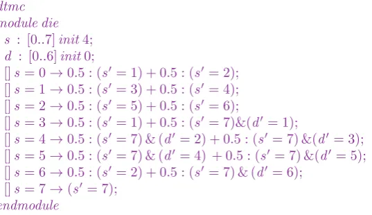
To introduce the syntax of the PRISM language, consider the simple proba-bilistic algorithm due to Knuth and Yao [12] for emulating a 6-sided die with a fair coin (see Figure 2) that can be found in the PRISM website4. The PRISM code corresponding to this algorithm can be seen in what follows.
4
Fig. 2.Graphical illustration of the 6-sided die with a fair coin
dtmc module die
s : [0..7]init4;
d : [0..6]init0;
[]s = 0→0.5 : (s′= 1) + 0.5 : (s′ = 2);
[]s = 1→0.5 : (s′= 3) + 0.5 : (s′ = 4);
[]s = 2→0.5 : (s′= 5) + 0.5 : (s′ = 6);
[]s = 3→0.5 : (s′= 1) + 0.5 : (s′ = 7)&(d′ = 1);
[]s = 4→0.5 : (s′= 7) & (d′= 2) + 0.5 : (s′ = 7) &(d′= 3);
[]s = 5→0.5 : (s′= 7) & (d′= 4) + 0.5 : (s′= 7) &(d′ = 5);
[]s = 6→0.5 : (s′= 2) + 0.5 : (s′ = 7) & (d′ = 6);
[]s = 7→(s′ = 7);
endmodule
The first thing to note is the reference to the kind of Markov chain being addressed. In this example, a Discrete-Time Markov Chain (DTMC) was used.
This PRISM specification is composed of a singlemodule, but if more than one module is presented an implicit parallel composition of them is considered as semantics [14]. This standard parallel composition can be customised to a new semantics by the use of asystem . . .endsystem section.
Inside a module, we can have local variables such as the s and d of this example. Both are natural numbers, ranging from 0..7 and 0..6, respectively. They need an initialisation. In this case, s is initially set to 4 andd to 0.
Thus the transition
[]s = 0→0.5 : (s′= 1) + 0.5 : (s′ = 2);
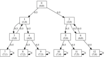
[image:8.595.224.392.220.315.2]may be read as follows: ifs= 0 holds, then this transition is fired. At this state, we have a 50-50% alternative to update the variable s. In the first alternative, the new value ofs is set to 1. Otherwise, 2. Figure 3 shows its Markov chain5.
Fig. 3.Markov chain for the 6-sided die
Finally, we can perform probabilistic analysis. For this example, we can calcu-late the probability of getting one of its 6-sides by writing the following property (standing for “What is the chance of eventuallysbecomes 7 anddbecomesx?”)
const int x;
P=? [F s= 7 &d=x]
where the constant x refers to a specific face of the die (x ∈ {1,2, . . . ,6}). In this example, the probability for each value ofx equals 16.67%.
4
WatchDog Transformation
The concurrent language CSP was extended to incorporate probabilistic and timed aspects in [16]. The probabilistic operator ⊞ was defined. However, this extension was entirely theoretical; no tool support was available at that time. In the work [8], a version of FDR was extended to handle the operator⊞.
Essentially, the standard CSPM notation (the machine-readable version of
CSP used by FDR) was augmented by the following new operator ([·∼·]). Let P andQ be CSP processes. Then
P m
(m+n) ⊞(mn+n) Q == P[m ∼n]Q
wherem andn are natural numbers.
5
The work [8], however, did not change the FDR algorithm to perform prob-abilistic analysis. Instead, FDR was extended to create a PRISM specification from a refinement assertion. This translation is briefly described as follows.
The WatchDog Transformation consists in analysing the probability with which a probabilistic CSP implementation (I) refines a non-probabilistic CSP specification process (S). In this paper it is enough to briefly present the Watch-Dog Transformationconcerning the traces semantics
S ⊑T I
It consists in mapping a specification process, sayS, to a watchdog process that monitors the traces of an implementation process, say I, to indicate whether or not I refinesS according to CSP’s traces semantics. Precisely, a watchdog process WDTS is defined such that it can perform a distinguished fail event
whenI performs a trace not allowed byS.
WDTS(i) = (
2
e∈αI∩A(i)•e→WDTS(after(i,e)))2
(
2
e∈αI\A(i)•e→fail →STOP)whereA(i) is calculated by FDR as part of the transformation.
The intention is that WDTS(i0) can perform any trace tr of I that S can
perform, but it can also perform events from the alphabet of I not allowed by
S/tr(after which it can only perform the eventfail ). Note that this definition of
WDT is expressed in terms of the alphabet,αI, of the implementation process
I which again must be calculated as part of the transformation. The original refinement check S ⊑T I is true precisely when WDTS(i0) ||αI I can never
perform the eventfail .
The previous CSP process in its LTS semantic form is translated into a PRISM specification based on a very few set of variables. The boolean variable
trace error matches the event fail . With this, theWatchDog Transformation is able to calculate a probability using the following formula6
Pmax=? [F trace error]
which mathematically corresponds to the following relation
S ⊑T I ⇔Pmax = 0% [F trace error]
The refinement holds exactly when the maximum probability of trace error
becomestrue is zero (or the eventfail never happens). Other interesting prob-abilities emerge when such a refinement can eventually fail. The interpretation of the above relation is thatPmax =? [F trace error] gives us the degree on which the refinementS ⊑T I may fail.
Thus, to explore the traces refinement to get useful probabilistic temporal analysis, one has to think of CSP processes as properties in such a way that the
6
traces refinement holds up to a certain point and then fail. From the temporal formula operatorF, the traces refinement must resemble a reachability analysis.
By default, the WatchDog Transformation creates an MDP PRISM speci-fication. But, if non-determinism may be ignored (for instance, in the 6-sided die example presented in Section 3), one can simply change the mdp directive to adtmc one in the PRISM specification. In such a case, the PRISM tool can calculate a single probability instead of a min/max probabilistic interval.
4.1 CSP to PRISM
To illustrate that the Markov chain generated by this approach is exactly what we need, we use the same example of Section 3. That algorithm written in CSP can be described as follows.
channel die:{1..6}
SixSidedDie=
let
S0 =S1 [1∼1]S2
S1 =S3 [1∼1]S4
S2 =S5 [1∼1]S6
S3 =S1 [1∼1]DIE(1)
S4 =DIE(2) [1∼1]DIE(3)
S5 =DIE(4) [1∼1]DIE(5)
S6 =S2 [1∼1]DIE(6)
DIE(x) =die.x →DIE(x)
within S0
To obtain the exact Markov chain as depicted in Figure 3, it suffices to apply theWatchDog Transformationon the following refinement
RUN(αSixSidedDie)⊑T SixSidedDie
The reason is simple. The process RUN(αSixSidedDie) can be refined by any process in the traces model and thus the PRISM variabletrace error is always
The generated PRISM code in what follows is naturally different from the one presented in Section 3. But its Markov chain is the same of Figure 3.
dtmc
moduleWATCHDOG pc: [0..1]init0;
trace error: bool init false;
[e2]pc! = 0→1 : (trace error′=true); //die.1
[e2]pc= 0→1 : (pc′=pc= 0?0 : 1);//die.1
[e3]pc! = 0→1 : (trace error′=true); //die.3
[e3]pc= 0→1 : (pc′=pc= 0?0 : 1);//die.3
[e4]pc! = 0→1 : (trace error′=true); //die.2
[e4]pc= 0→1 : (pc′=pc= 0?0 : 1);//die.2
[e5]pc! = 0→1 : (trace error′=true); //die.4
[e5]pc= 0→1 : (pc′=pc= 0?0 : 1);//die.4
[e6]pc! = 0→1 : (trace error′=true); //die.6
[e6]pc= 0→1 : (pc′=pc= 0?0 : 1);//die.6
[e7]pc! = 0→1 : (trace error′=true); //die.5
[e7]pc= 0→1 : (pc′=pc= 0?0 : 1);//die.5
endmodule moduleP0
pc0: [0..13]init0;
[]pc0= 0→0.5 : (pc0′= 1) + 0.5 : (pc′0= 2);// prob.0
[]pc0= 1→0.5 : (pc0′= 3) + 0.5 : (pc′0= 4);// prob.1
[]pc0= 2→0.5 : (pc0′= 5) + 0.5 : (pc′0= 6);// prob.2
[]pc0= 3→0.5 : (pc0′= 1) + 0.5 : (pc′0= 7);// prob.3
[]pc0= 4→0.5 : (pc0′= 8) + 0.5 : (pc′0= 9);// prob.4
[]pc0= 5→0.5 : (pc0′= 10) + 0.5 : (pc′0= 11);// prob.5
[]pc0= 6→0.5 : (pc0′= 2) + 0.5 : (pc′0= 12);// prob.6
[e2]pc0= 7→1 : (pc0′=pc0= 7?7 : 13);//die.1
[e3]pc0= 9→1 : (pc0′=pc0= 9?9 : 13);//die.3
[e4]pc0= 8→1 : (pc0′=pc0= 8?8 : 13);//die.2
[e5]pc0= 10→1 : (pc0′=pc0= 10?10 : 13);//die.4
[e6]pc0= 12→1 : (pc0′=pc0= 12?12 : 13);//die.6
[e7]pc0= 11→1 : (pc0′=pc0= 11?11 : 13);//die.5
endmodule system
WATCHDOG || P0
endsystem
Instead of the variables s and d, we have integer variables whose prefix start with pc (resembling the program counter of an assembly code and match the LTS state) and the trace error boolean variable. Therefore, if one is interested to analyse this generated PRISM code directly, instead of using the formula
P =? [F s = 7 &d =x], it is necessary to useP =? [F pc0 =y] where y must assume one of the values 7, 8, 9, 10, 11, or 12, corresponding to the events
die.1,. . . ,die.6, which can be detected by simply reading the comments. Fortunately, we do not need to know anything about thepc variables, nor the above automatically generated PRISM specification. Instead, we just have to formulate the appropriate traces refinement directly in CSP terms and check forPmax =? [F trace error]. For this example, the CSP refinement could be
Prop⊑T SixSidedDie
5
Using probabilities in RoboChart
In this section we present our strategy that allows probabilistic analysis of RoboChart models. We first introduce the use of the probabilistic RoboChart operator and then the extended RoboChart probabilistic semantics.
5.1 The RoboChart probabilistic operator
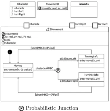
To create RoboChart models with probabilistic properties, we have to use a specific operator: Probabilistic Junction (P). To illustrate its usage, we now consider an extension of the state machine of the RoboChart model presented in Section 2. We consider that the robot is equally likely to turn to the right and to the left. This new model is shown in Figure 4.
[image:12.595.215.401.302.490.2]Probabilistic Junction
Fig. 4.RoboChart: obstacle detection with probabilities.
5.2 Dealing with probabilities
To extend the semantics of RoboChart models to deal with probability aspects, we have to consider the CSP probabilistic operator⊞to define the semantics of P, instead of internal choices. Leth| · |ibe this extended semantics.
To be able to analyse probabilistic RoboChart models, it suffices to apply the strategy presented in Section 4. That is, take a RoboChart modelR, formulate the desired property about R as a CSP specification S, apply the WatchDog Transformationon the refinement
S ⊑T h|R|i
and use the PRISM model checker using the single LTL formula
Pmax=? [F trace error]
Finally, interpret the result of the above formula as it is related to S 6⊑T h|R|i.
6
Case Study
In this section, we present a RoboChart model with probabilistic primitives. Furthermore, we also discuss some probabilistic analysis of the RoboChart model that the robotic engineers are now able to do.
6.1 Obstacle Detection
In this section we just illustrate the kind of analysis we can perform on our running example from Section 5.1.
We can use as property the following CSP specification.
Prop=moveCall →moveRet →SMovement obstacle→
SMovement turnRight→STOP
After performing the refinement
Prop⊑T Obstable Detection
and checking for the probability ofPmax =? [F trace error] we get 100%, indi-cating that (by the probabilistic complement) such a refinement does not hold.
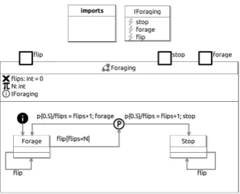
6.2 Foraging Robot
Fig. 5.RoboChart model
to ignore the outcome of the device. Finally, the robot considers only a limited number of times whether to continue foraging (see Figure 5).
The initial transition inForaging leads to state Forage, in which a number of transitions can be taken. If a flip is allowed (represented by the occurrence of the event flip), the robot may ignore the randomising device and remain in the Forage state. Another possible transition from Forage happens when the event flip occurs and the number of choices has not been exhausted, given by (flips<N). The constantNrepresents the maximum number of choices. In this case, the control proceeds to a probabilistic junction between two equally likely alternatives. One alternative is to move into theStopstate, which it signals with the stop event. The other is to return to the Forage state, signalling this with theforageevent. In both cases, the value of flips is incremented (flips = flips+1). This is used by the machine to keep track of the number of choices made.
There is only one transition available in the Stopstate: theflip event keeps the controller inStop; this transition is included to model the fact that flip occurs in every time step, even when the controller has terminated.
The CSP refinement property to check this model can be written as:
Prop= (
2
e:{flip,forage} •e→Prop)2stop →STOP
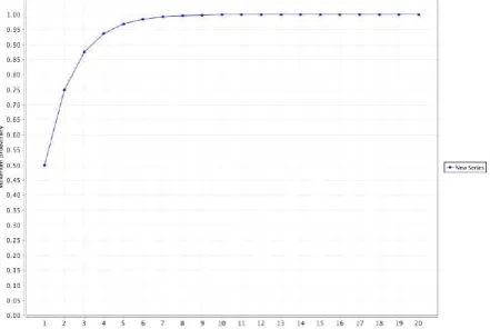
By varying theNfrom 1 to 20 we get the graph depicted in Figure 6.
7
Conclusions
Fig. 6.Graph for Foraging Robot model plotting N from 1 to 20
of a refinement such asP ⊑T Q, whereQ is the probabilistic CSP specification automatically generated by RoboTool andP is some property of interest.
The strategy reported in this paper has two main advantages over other attempts found in literature. The first is that it is based on CSP refinement and not in LTL model checking. This allows a more closer analysis style as already present in RoboChart. The second is that all data structures and functional language already available in CSP is inherited by the automatically generated PRISM specification. This is very interesting because it is hard to find rich data structures as well as a readable PRISM specification in literature.
One drawback of our strategy is that we never get a parameterised PRISM specification. But we can generate several models, each one corresponding to the values of the parameters being analysed. This is what the PRISM tool does directly from a parameterised PRISM specification.
Some works have been proposed for analyzing stochastic properties of robotic systems. In [13], probabilistic analysis are performed focusing on the robotic control software, ignoring the environment. It manually captures probabilistic state machines (using the PRISM language) of swarm systems from [15] in order to check specific properties in PCTL. No formal semantics is reported in this work. Probabilistic properties of swarm robotic models are also verified in [17]. It uses the process algebra Bio-PEPA [2] for modelling such models, which can be mapping to PRISM models by the Bio-PEPA suite of software tools.
We are working on another route to analysis of RoboChart models. This route goes from RoboChart to PRISM’s Reactive Modules formalism via prob-abilistic Statecharts [10], and will give an alternative way of establishing proba-bilistic temporal properties. This translation is being built from metamodels of RoboChart, probabilistic Statecharts, and Reactive Modules, with the transla-tion carried out using the Epsilon model transformatransla-tion tool7. Our translation
7
can also be expressed in Unifying Theories of Programming [9] as a Galois con-nection between Statecharts and Reactive Modules, suggesting a bidirectional transformation in Epsilon, supporting traceability of analysis results and coun-terexamples, and giving a formal way of verifying the translation using a seman-tics based on probabilistic predicate transformers in the style of McIver [19]. An interesting question is whether this more direct route will lead to models with different analysis performance in the PRISM tool.
Our translations will allow the use of more than just PRISM: the Reactive Modules formalism is also used for input to the MRMC and Storm model check-ers, amongst othcheck-ers, and a dialect of probabilistic CSP is used for input to the PAT model checker [24]. We plan to explore the use of these alternatives and compare their performance on benchmarks that we will establish in robotic and autonomous control.
Finally, we plan to verify the results used in this paper, and in particular, theWatchDog Transformation as an implementation technique, using the CSP theories in Isabelle/UTP [5, 7, 6].
Acknowledgements.
This research was partially supported by INES 2.0, CAPES, FACEPE (grants PRONEX APQ 0388-1.03/14 and APQ-0399-1.03/17), and CNPq (grant 465614/ 2014-0). We would like to thank Andr´e Didier and Matheus Santana.
References
1. C. Baier and Joost-Pieter Katoen. Principles of Model Checking (Representation and Mind Series). The MIT Press, 2008.
2. F. Ciocchetta and J. Hillston. Bio-pepa: a framework for the modelling and analysis of biological systems, 2008.
3. C. Dehnert, S. Junges, Joost-Pieter Katoen, and M. Volk. A storm is coming: A modern probabilistic model checker. In CAV (2), volume 10427 ofLNCS, pages 592–600. Springer, 2017.
4. L. Fernandes, V. Custodio, G. Alves, and M. Fisher. A rational agent controlling an autonomous vehicle: Implementation and formal verification. InEPTCS, pages 35–42, 2017.
5. S. Foster and J. Woodcock. Unifying theories of programming in isabelle. In ICTAC Training School on Software Engineering, volume 8050 of LNCS, pages 109–155. Springer, 2013.
6. S. Foster and J. Woodcock. Mechanised theory engineering in isabelle. In Depend-able Software Systems Engineering, volume 40 of NATO Science for Peace and Security Series, D: Information and Communication Security, pages 246–287. IOS Press, 2015.
7. S. Foster, F. Zeyda, and J. Woodcock. Isabelle/utp: A mechanised theory engi-neering framework. InUTP, volume 8963 ofLNCS, pages 21–41. Springer, 2014. 8. M. Goldsmith. Csp: The best concurrent-system description language in the
world-probably! InCommunicating Process Architectures, pages 227–232, 2004.
10. David N. Jansen, Holger Hermanns, and Joost-Pieter Katoen. A probabilistic ex-tension of UML statecharts. In Werner Damm and Ernst-R¨udiger Olderog, editors, Formal Techniques in Real-Time and Fault-Tolerant Systems, 7th International Symposium, FTRTFT 2002, Co-sponsored by IFIP WG 2.2, Oldenburg, Germany, September 9-12, 2002, Proceedings, volume 2469 of Lecture Notes in Computer Science, pages 355–374. Springer, 2002.
11. Joost-Pieter Katoen, Ivan S. Zapreev, Ernst Moritz Hahn, Holger Hermanns, and David N. Jansen. The ins and outs of the probabilistic model checker mrmc. Perform. Eval., 68(2):90–104, February 2011.
12. D. Knuth and A. Yao.Algorithms and Complexity: New Directions and Recent Re-sults, chapter The complexity of nonuniform random number generation. Academic Press, 1976.
13. Fisher M. Konur S., Dixon C. Formal verification of probabilistic swarm be-haviours.
14. M. Kwiatkowska, G. Norman, and D. Parker. Prism 4.0: Verification of probabilistic real-time systems. In Ganesh Gopalakrishnan and Shaz Qadeer, editors,Computer Aided Verification, pages 585–591. Springer Berlin Heidelberg, 2011.
15. W. Liu, Alan F. T. Winfield, and Jin Sa. Modelling swarm robotic systems : A case study in collective foraging. 2007.
16. Gavin Lowe. Probabilistic and prioritized models of timed CSP.Theoretical Com-puter Science, 138(2):315 – 352, 1995.
17. D. Latella M. Dorigo M. Massink, M. Brambilla and M. Birattari. On the use of bio-pepa for modelling and analysing collective behaviours in swarm robotics. page 201228.
18. M. Fisher M. Salem J. Saunders K. L. Koay M. Webster, C. Dixon and K. Dauten-hahn. Formal verification of an autonomous personal robotic assistant. InAAAI Spring Symposium Series, page 7479, 2014.
19. A. McIver. Quantitative refinementand model checking for the analysis of proba-bilistic systems. InFM, volume 4085 ofLNCS, pages 131–146. Springer, 2006. 20. A. Miyazawa, A. Cavalcanti, P. Ribeiro, W. Li, J. Woodcock, and
J. Timmis. RoboChart Reference Manual. University of York, 2016. https://www.cs.york.ac.uk/circus/RoboCalc/assets/RoboChart-manual.pdf. 21. A. Miyazawa, P. Ribeiro, W. Li, A. Cavalcanti, and J. Timmis. Automatic property
checking of robotic applications. InIROS, pages 3869–3876, 2017.
22. P. Ribeiro, A. Miyazawa, W. Li, A. Cavalcanti, and J. Timmis. Modelling and verification of timed robotic controllers. InIFM 2017, pages 18–33, 2017. 23. A.W. Roscoe. Understanding Concurrent Systems. Springer-Verlag.
24. Songzheng Song, Jun Sun, Yang Liu, and Jin Song Dong. A model checker for hierarchical probabilistic real-time systems. InCAV, volume 7358 ofLNCS, pages 705–711. Springer, 2012.
25. A. Boulgakov A.W. Roscoe T. Gibson-Robinson, P. Armstrong. FDR3 — A Mod-ern Refinement Checker for CSP. In Erika brahm and Klaus Havelund, editors, Tools and Algorithms for the Construction and Analysis of Systems, volume 8413 ofLecture Notes in Computer Science, pages 187–201, 2014.
26. M. Tribastone. The pepa plug-in project, 2009.