This is a repository copy of
Estimation and forecasting in vector autoregressive moving
average models for rich datasets
.
White Rose Research Online URL for this paper:
http://eprints.whiterose.ac.uk/144638/
Version: Accepted Version
Article:
Dias, G.F. and Kapetanios, G. (2018) Estimation and forecasting in vector autoregressive
moving average models for rich datasets. Journal of Econometrics, 202 (1). pp. 75-91.
ISSN 0304-4076
https://doi.org/10.1016/j.jeconom.2017.06.022
© 2017 Elsevier. This is an author-produced version of a paper subsequently published in
Journal of Econometrics. Uploaded in accordance with the publisher's self-archiving policy.
Article available under the terms of the CC-BY-NC-ND licence
(https://creativecommons.org/licenses/by-nc-nd/4.0/)
[email protected] https://eprints.whiterose.ac.uk/ Reuse
This article is distributed under the terms of the Creative Commons Attribution-NonCommercial-NoDerivs (CC BY-NC-ND) licence. This licence only allows you to download this work and share it with others as long as you credit the authors, but you can’t change the article in any way or use it commercially. More
information and the full terms of the licence here: https://creativecommons.org/licenses/
Takedown
If you consider content in White Rose Research Online to be in breach of UK law, please notify us by
Estimation and Forecasting in Vector Autoregressive Moving
Average Models for Rich Datasets
Gustavo Fruet Dias∗
Department of Economics and Business Economics, Aarhus University CREATES
George Kapetanios King’s College London
Abstract
We address the issue of modelling and forecasting macroeconomic variables using rich datasets by adopting the class of Vector Autoregressive Moving Average (VARMA) models. We overcome the estimation issue that arises with this class of models by im-plementing an iterative ordinary least squares (IOLS) estimator. We establish the con-sistency and asymptotic distribution of the estimator for weak and strong VARMA(p,q) models. Monte Carlo results show that IOLS is consistent and feasible for large systems, outperforming the MLE and other linear regression based efficient estimators under al-ternative scenarios. Our empirical application shows that VARMA models are feasible alternatives when forecasting with many predictors. We show that VARMA models outperform the AR(1), ARMA(1,1), Bayesian VAR, and factor models, considering dif-ferent model dimensions.
JEL classification numbers: C13, C32, C53, C63, E0
Keywords: VARMA, weak VARMA, Iterative ordinary least squares (IOLS) estima-tor, Asymptotic contraction mapping, Forecasting, Rich and Large datasets.
Acknowledgments: This paper previously circulated under the title “Forecasting Medium and Large Datasets with Vector Autoregressive Moving Average (VARMA) Models”. We are indebted to Emmanuel Guerre, Cristina Scherrer and the seminar participants at Queen Mary (Econometrics Reading Group), the 14th Brazilian Time Series and Econometrics School (Gramado, Aug 2011), the Econometric Society Aus-tralasian Meeting (Adelaide, July 2011), the Royal Economic Society Annual Conference (Royal Holloway, University of London, April 2011) and the 4th International Conference on Computational and Financial Econometrics (London, Dec 2010).
Gustavo Fruet Dias acknowledges support from CREATES - Center for Research in Econometric Analy-sis of Time Series (DNRF78), funded by the Danish National Research Foundation. The usual disclaimer applies.
∗Corresponding author at: Department of Economics and Business Economics, Aarhus University,
1
Introduction
The use of large arrays of economic indicators to forecast key macroeconomic variables
has become very popular recently. Economic agents consider a wide range of information
when they construct their expectations about the behaviour of macroeconomic variables
such as interest rates, industrial production, and inflation. In the past several years, this
information has become more widely available through a large number of indicators that
aim to describe different sectors and fundamentals from the whole economy. To improve
forecast accuracy, large sized datasets that attempt to replicate the set of information used
by agents to make their decisions are incorporated into econometric models.
For the past twenty years, macroeconomic variables have been forecasted using vector
autoregression (VAR) models. This type of model performs well when the number of
vari-ables in the system is relatively small. When the number of varivari-ables increases, however,
the performance of VAR forecasts deteriorates very fast, generating the so-called “curse of
dimensionality”. In this paper, we propose the use of vector autoregressive moving average
(VARMA) models, estimated with the iterative ordinary least squares (IOLS) estimator,
as a feasible method to address the “curse of dimensionality” on medium and large sized
datasets and improve forecast accuracy of macroeconomic variables. To the best of our
knowledge, the VARMA methodology has never been applied to medium and large sized
datasets, as we do in this paper.
VARMA models have been studied for the past thirty years, but they have never been
as popular as VAR models because of estimation and specification issues. Despite having
attractive theoretical properties, estimation of VARMA models remains a challenge. Linear
estimators (Hannan and Rissanen (1982), Hannan and Kavalieris (1984), Dufour and Jouini
(2014), among others) and Bayesian methods (Chan, Eisenstat, and Koop (2016)) have
been proposed in the literature as a way to overcome the numerical difficulties posed by
the efficient maximum-likelihood estimator. We address the estimation issue and hence
contribute to this literature by proposing the use of the IOLS estimator that is feasible for
high-dimensional VARMA models.
Other methodologies have been proposed in the literature to deal with the “curse of
dimensionality”. We can divide them mainly in two groups of models. The first aims
to overcome the dimensionality issue by imposing restrictions on the parameter matrices
point out the following classes of models: Bayesian VAR (BVAR) (De Mol, Giannone, and
Reichlin (2008) and Ba´nbura, Giannone, and Reichlin (2010)); Ridge (De Mol, Giannone,
and Reichlin (2008)); reduced rank VAR (Carriero, Kapetanios, and Marcellino (2011));
and Lasso (De Mol, Giannone, and Reichlin (2008) and Tibshirani (1996)). The second
group of models dealing with the “curse of dimensionality” reduces the dimension of the
dataset by constructing summary proxies from the large dataset. Chief among these models
is the class of factor models. The seminal works in this area are Forni, Hallin, Lippi, and
Reichlin (2000) and Stock and Watson (2002a,b). Common factor models improve forecast
accuracy and produce theoretically well-behaved impulse response functions, as reported
by De Mol, Giannone, and Reichlin (2008) and Bernanke, Boivin, and Eliasz (2005).
VARMA models are able to capture two important features from these two groups of
models. The first is the reduction of the model dimensionality, achieved by setting some
elements of the parameter matrices to zero following uniqueness requirements. This
pro-duces parameter matrices which are not full rank, resembling the reduced rank VAR model
of Carriero, Kapetanios, and Marcellino (2011). Furthermore, VARMA models
parsimo-niously account for sample correlation profiles of different shapes than the geometrically
declining sinusoids associated with the VAR models. The second is the relationship
be-tween VARMA models and factor representations of a vector stochastic process. If the
latent common factors follow either a finite VAR or VARMA processes, then the observed
series will have a VARMA representation (Dufour and Stevanovi´c (2013)). This fact
rein-forces the use of VARMA models as a suitable framework to forecast key macroeconomic
variables using potentially many predictors. Additionally, VARMA models are closed under
linear transformation and marginalization (see L¨utkepohl (2007, Section 11.6.1)), providing
additional flexibility and potentially better forecast performance.
With regard to the theory, we establish the consistency and asymptotic distribution
of the IOLS estimator for the weak and strong VARMA(p,q) models. Strong VARMA
models have innovations that are independently identically distributed (i.i.d.), while the
disturbances of the weak VARMA models are only uncorrelated. Our asymptotic results
are obtained under mild assumptions using the asymptotic contraction mapping framework
of Dominitz and Sherman (2005). We conduct an extensive Monte Carlo study, considering
different system dimensions, sample sizes, weak and strong innovations, eigenvalues
IOLS estimator has a good finite sample performance when compared to alternative
esti-mators, such as the efficient maximum-likelihood (MLE) estimator, and important linear
competitors. Specifically, the IOLS estimator performs well in a variety of scenarios such as
small sample size; the eigenvalues associated with the parameter matrices are near-to-zero;
and high-dimensional systems.
In the empirical part of the paper, we focus on forecasting three key macroeconomic
variables: industrial production, interest rate, and CPI inflation using potentially large sized
datasets. As in Carriero, Kapetanios, and Marcellino (2011), we use the 52 US
macroeco-nomic variables taken from the dataset provided by Stock and Watson (2006) to construct
systems with five different dimensions: 3, 10, 20, 40, and 52 variables. By doing that, we
are able to evaluate the tradeoff between forecast gains by incorporating more information
(large sized datasets) and the estimation cost associated with it. Additionally, the
differ-ent system dimensions play the role of robustness check. We show that VARMA models
are strong competitors and produce more accurate forecasts than the benchmark models
(AR(1), ARMA(1,1), BVAR, and factor models) in different occasions. This conclusion
holds for different system sizes and horizons.
The paper is structured as follows. In Section 2, we discuss the properties and
identi-fication of VARMA models and derive the IOLS estimator. In Section 3, we establish the
consistency and asymptotic distribution of the IOLS estimator considering the general weak
and strong VARMA(p,q) models. In Section 4, we address the consistency and efficiency
of VARMA models estimated with the IOLS procedure through a Monte Carlo study. In
Section 5, we display the results of our empirical application. The proofs and tables are
relegated to an Appendix. An online Supplement presents proofs for the auxiliary Lemmas,
the entire set of tables with results for the Monte Carlo and the empirical studies, and
further discussion on selected topics.
2
VARMA Models, Identification, and Estimation
Proce-dures
model, a general nonstandard VARMA(p,q) model where the means have been removed,1
A0Yt=A1Yt−1+A2Yt−2+...+ApYt−p+M0Ut+M1Ut−1+...+MqUt−q, (1)
where the disturbances Ut = (u1,t, u2,t, ..., uK,t)′ are assumed to be a zero-mean sequence
of uncorrelated random variables (weak white noise process) with a nonsingular (K×K) covariance matrix Σu, andY has dimension (K×1). Our baseline model is assumed to be
stable and invertible.2
2.1 Identification and Uniqueness
The issue of identifying unique parameterizations of VARMA models has been an important
topic of study in econometrics and statistics (Hannan (1969, 1976), Akaike (1974, 1976),
Hannan and Kavalieris (1984), Hannan and Deistler (1988), among others). This follows
because nonstandard VARMA models require restrictions on the parameter matrices to
ensure that the model is uniquely identified. To formally define uniqueness of a VARMA
representation, define the lag polynomials A(L) = A0 −A1L−A2L2 −...−ApLp and
M(L) =M0+M1L+M2L2+...+MqLq, whereLis the usual lag operator. More specifically,
we say that a model is unique if there is only one pair of stable and invertible polynomials
A(L) and M(L), respectively, which satisfies the canonical MA representation
Yt=A(L)−1M(L) = Θ (L)Ut= ∞
X
i=0
ΘiUt−i, (2)
for a given Θ (L) operator. In contrast to the reduced form VAR models, setting A0 = M0 = IK is not sufficient to ensure a unique VARMA representation. Uniqueness of (1)
is guaranteed by imposing restrictions on the A(L) and M(L) operators in that these operators are unique left-coprime, i.e. the only feasible left divisor of [A(L) :M(L)] is the unimodular operator given by the identity matrix.3
A number of different strategies can be implemented to obtain unique VARMA
repre-sentations, such as the extended scalar component approach of Athanasopoulos and Vahid
1We adopt the terminology in L¨utkepohl, 2007, p. 448 and call a VARMA representation nonstandard
whenA0 andM0 are allowed to be nonidentity invertible matrices. IfA0=M0=IK, we call it a standard VARMA model.
2A general VARMA(p,q) is considered stable and invertible if det A
0−A1z−A2z2−...−Apzp 6= 0
f or|z| ≤1 and det M0+M1z+M2z2+...+Mqzq6= 0f or|z| ≤1 hold, respectively.
(2008), the final equations form (see L¨utkepohl, 2007, pg.362) and the Echelon form
trans-formation (Hannan and Kavalieris (1984), Poskitt (1992), L¨utkepohl and Poskitt (1996),
among others). Although Athanasopoulos, Poskitt, and Vahid (2012) show that scalar
com-ponents perform slightly better than the Echelon form methodology in empirical exercises,
the authors argue that the latter has the advantage of having a simpler identification
proce-dure. More specifically, the Echelon form identification strategy can be fully automated and
provides a more parsimonious parametrization, when compared to final equations. These
are highly desired features when modelling medium and large systems. In this paper, we
implement the Echelon form transformation as a way to impose uniqueness in both Monte
Carlo and empirical applications. Nevertheless, because the three identification strategies
(scalar components, final equations form, and Echelon form) impose uniqueness through
a set of linear restrictions on the A(L) and M(L) operators, the IOLS estimator can be directly implemented no matter which identification strategy the researcher chooses.
A general VARMA model such as the one stated in (1) is considered to be in its Echelon
form if the conditions stated in equations (3), (4), (5), and (6) are satisfied (see L¨utkepohl,
2007, p. 452 and L¨utkepohl and Poskitt (1996) for more details):
pki :=
min (pk+ 1, pi) for k≥i
min (pk, pi) fork < i,
fork, i= 1, ..., K, (3)
αkk(L) = 1− pk
X
j=1
αkk,jLj fork= 1, ..., K, (4)
αki(L) =− pk
X
j=pk−pki+1
αki,jLj fork6=i, (5)
mki(L) = pk
X
j=0
mki,jLj, fork, i= 1, ..., K with M0=A0, (6)
where A(L)=[αki]k,i=1,...,K and M(L)=[mki]k,i=1,...,K are, respectively, the operators from
the autoregressive and moving average components of the VARMA process; thepkinumbers
specify the free coefficients in the operator αki(L) for i 6= k from the A(L) polynomial;
and the argumentspk withk= 1, ..., K are Kronecker indices which specify the maximum
degrees in each row of bothA(L) andM(L) polynomials. We definep= (p1, p2, ..., pK)′ as
the vector collecting the Kronecker indices (Section 5.1 discusses alternative procedures to
The Echelon form formulae in (3) to (6) deliver the necessary and sufficient restrictions
for the unique identification of the VARMA models (Hannan and Deistler, 1988, Chapter
2). Notably, the Echelon representation allows the baseline model in (1) to be rewritten as
Yt= (IK−A0) (Yt−Ut) +A1Yt−1+A2Yt−2+...+ApYt−p+Ut+M1Ut−1+...+MqUt−q, (7)
where (Yt−Ut) = A−01{
Pp
i=1AiYt−i+Pqi=1MiUt−i} is uncorrelated with Ut. A compact
notation of (7) reads
vec (Y) = X′⊗IKvec (B) + vec (U), (8)
where B = [(IK −A0), A1, ..., Ap, M1, ..., Mq] with dimension (K ×K(p +q + 1)); X =
(Xq¯+1, ..., XT) is the matrix of regressors with dimension (K(p+q + 1)×T −q), where¯
¯
q = max{p, q} and Xt = vec(Yt−Ut, Yt−1, ..., Yt−p, Ut−1, ..., Ut−q); Y = (Yq¯+1, ..., YT) has
dimension (K ×T −q); and¯ U = (U¯q+1, ..., UT) is a (K ×T −q) matrix of disturbances.¯
Note that by setting the dimensions of the X and Y matrices as (K(p+q+ 1)×T −q)¯ and (K×T−q), respectively, we explicitly highlight the fact that we lose ¯¯ q observations in finite sample. We obtain the free parameters in the model (excluding the distinct covariance
parameters) by rewriting vec (B) into the product of a K2(p+q+ 1)×n deterministic matrixR and a (n×1) vectorβ,
vec (Y) = X′⊗IKRβ+ vec (U), (9)
where n denotes the number of free parameters in B, and the (n×1) vector β concate-nates these parameters. The Echelon restrictions imply a unique full-rank column matrix
Rand, provided that Σu is nonsingular, ensure thatrank{R′[E(XtXt′)⊗IK]R}=n
(Du-four and Jouini (2005, 2014)). It is still possible to impose additional zero restrictions (data
dependent) while keeping the model uniquely identified and hence obtain a more
parsimo-nious model (see L¨utkepohl and Poskitt, 1996, p. 73). This follows because a Kronecker
index only gives the maximum row degree, and hence not all operators in the kth row of
[A(L) :M(L)] need to have the same degree aspk. As an example, consider a VARMA(1,1)
Echelon form reads
1 0 0
a21,0 1 0
a31,0 0 1
Yt=
a11,1 0 0
0 0 0
0 0 0
Yt−1+
1 0 0
a21,0 1 0
a31,0 0 1
Ut+
m11,1 m12,1 m13,1
0 0 0
0 0 0
Ut−1. (10)
While the zero restrictions imposed in (10) are those required to meet the restriction
im-posed by the canonical structure, further restrictions that simplify the model could be added
(e.g. a21,0 = a31,0 = m12,1 = m13,1 = 0) without affecting the uniqueness of the VARMA
representation. Throughout this entire study, we refrain from adding these additional
re-strictions and restrict ourselves to the ones implied from (3) to (6). Furthermore, we always
consider the Echelon forms that yield VARMA models that cannot be partitioned into
smaller independent systems.
Finally, it is important to note that the VARMA representation in (1) is not a structural
VARMA (SVARMA) model in its classical definition (see Gourieroux and Monfort (2015)),
because (1) is not necessarily driven by independent (or uncorrelated) shocks. To construct
impulse response functions, which depend on the structural shocks, additional identification
restrictions to the ones required for uniqueness are necessary. In particular, as noted by
Gourieroux and Monfort (2015), the structural shocks can usually be derived by imposing
restrictions either on the contemporaneous correlation among the innovations in (1) (see
the so-called B-model in L¨utkepohl, 2007, p. 362 and the general identification theory in
Rubio-Ram´ırez, Waggoner, and Zha (2010)), or on the long-run impact matrix of the shocks
(Blanchard and Quah (1989)), or by imposing sign restrictions on some impulse response
functions (Uhlig (2005)). This identification issue is common to both VARMA and VAR
models and has been primarily explored in the context of VAR models.
2.2 Estimation
VARMA models, similar to their univariate (ARMA model) counterparts, are usually
es-timated using MLE procedures. Provided that the model in (1) is uniquely identified and
disturbancesUtare normally distributed, MLE delivers consistent and efficient estimators.
Although MLE seems to be very powerful at first glance, it presents serious problems when
IOLS procedure in the spirit of Spliid (1983), Hannan and McDougall (1988) and
Kapetan-ios (2003).
The IOLS framework consists of computing ordinary least squares (OLS) estimates of
the parameters using estimates of the latent regressors. These regressors are computed
recursively at each iteration using the OLS estimates. Using the invertibility condition, we
can express a finite VARMA model as an infinite VAR,Yt= ∞
P
i=1
ΠiYt−i+Ut. We compute
consistent estimates of Ut, denoted as Ubt0, by truncating the infinite VAR representation
using some lag order, ˜p, that minimizes some criterion. Following the results in Ng and Perron (1995) and Dufour and Jouini (2005), choosing ˜p proportional to ln (T) delivers consistent estimates of Ut, so that Ubt0 = Yt−
˜
p
P
i=1
b
ΠiYt−i.4 Substitute Ubt0 into the matrix
X in (9) and denote it Xb0. Note that both Xb0 and vec (Y) change their dimensions to (K(p+q+ 1)×T−q¯−p) and (K(T˜ −q¯−p)˜ ×1), respectively. This happens exclusively on this first iteration, because ˜p observations are lost on the VAR(˜p) approximation of Ut.
The first iteration of the IOLS estimator is obtained by computing the OLS estimator from
the modified version of (9),
b
β1 =hR′Xb0Xb0′⊗IK
Ri−1R′Xb0⊗IK
vec(Y). (11)
It is relevant to highlight that the first step of the IOLS estimator is the two-stage
Hannan-Rissanen (HR) algorithm formulated in Hannan and Hannan-Rissanen (1982), and for which Dufour
and Jouini (2005) show the consistency and asymptotic distribution.
We are now in a position to use βb1 to recover the parameter matrices Ab1
0, ...,Ab1p,
c
M1
1, ...,Mcq1 and a new set of residuals Ub1=
b
U1
1,Ub21, ...,UbT1
by recursively applying
b
Ut1=Yt−
h b
A10i−1hAb11Yt−1−...−Ab1pYt−p−Mc11Ubt1−1−...−Mcq1Ubt1−q
i
, fort= 1, ..., T, (12)
whereYt−ℓ =Ubt1−ℓ= 0 for all ℓ≥t. Setting the initial values to zero when computing the
residuals recursively on any iteration is asymptotically negligible (see Lemma 2). Note that
the superscript on the parameter matrices refers to the iteration in which those parameters
are computed, and the subscript is the usual lag order. We compute the second iteration of
the IOLS procedure by pluggingUbt1 into (9) yielding Xb1. Note that Xb1 = (Xbq1¯+1, ...,XbT1),
4Lemmas 4.1 and 4.2 in Ng and Perron (1995) show that determining the truncation lag proportional
to ln (T) guarantees that the difference between the residuals from the truncated VAR model and the ones obtained from the infinite VAR process isop
whereXb1
t = [Yt−Ubt1, Yt−1, ..., Yt−p,Ubt1−1, ...,Ubt1−q]′, is a function of the estimates obtained
in the first iteration: βb1. Similarly as in (11), we obtain βb2 and its correspondent set of residuals recursively as in (12). The jth iteration of the IOLS estimator is thus given by
b
βj =hR′Xbj−1Xbj−1′⊗IK
Ri−1R′Xbj−1⊗IK
vec(Y). (13)
We stop the IOLS algorithm when estimates ofβconverge. We assume thatβbj converges
ifkUbj−Ubj−1k≤ǫholds from some exogenously defined criterionǫ, wherek.kaccounts for the Frobenius norm. If the IOLS fails to converge, we adopt the consistent HR estimator,
b
β1, given in (11). The maximum number of iterations is set to 1,000 andǫ= 10−5. We also notice from our simulations that sample size, number of free parameters, system dimension,
and the values ofβ play an important role on the convergence rates of the IOLS estimator. In general, we find that convergence rates increase monotonically withT (see discussion in Sections 3 and 4).
3
Theoretical Properties
This section provides theoretical results regarding the consistency and the asymptotic
dis-tribution of the IOLS estimator. A previous attempt to establish these results have been
made by Hannan and McDougall (1988). They prove the consistency of the IOLS estimator
considering the univariate ARMA(1,1) specification, but no formal result is provided for the
asymptotic normality. Overall, this section differs from the work of Hannan and McDougall
(1988) in important ways. First, we derive the consistency and the asymptotic normality
for the general weak and strong VARMA(p,q) models; and second, our theory explicitly
accounts for the effects of setting initial values equal to zero when updating the residuals
on each iteration.
Similarly as in Section 2, we define our baseline weak VARMA(p,q) model expressed in
its Echelon form as in (14) and its more compact notation in (15):
A0Yt=A1Yt−1+A2Yt−2+...+ApYt−p+A0Ut+M1Ut−1+...+MqUt−q, (14)
Yt= Xt′⊗IKRβ+Ut, (15)
We base our asymptotic results on the general theory for iterative estimators developed
by Dominitz and Sherman (2005).5 Their approach relies on the concept of the Asymptotic
Contraction Mapping (ACM). Denote (B, d) as a metric space where B is the closed ball centered in β and d is a distance function; (Ω,A,P) is a probability space, where Ω is a sample space, A is a σ-field of subsets of Ω and P is the probability measure on A; and KTω(.) is a function defined onB, withω∈Ω. From the definition in Dominitz and Sherman, 2005, p. 841,“The collection {KTω(.) :T ≥1, ω ∈Ω} is an ACM on (B, d) if there exist a constant c ∈[0,1) that does not depend on T or ω, and sets {AT} with each AT ⊆Ω and
PAT → 1 as T → ∞, such that for each ω ∈ AT, KTω(.) maps B to itself and for all
x, y∈B,d(Kω
T (x), KTω(y))≤cd(x, y)”. As pointed out by Dominitz and Sherman (2005),
if a collection is an ACM, then it will have a unique fixed point in (B, d), where the fixed point now depends on the sample characteristics, i.e. T and ω. Additionally, their ACM definition nests the case where the population mapping is a fixed deterministic function
(Dominitz and Sherman, 2005, p. 840).
Definition 1 (General Mapping) We define the sample mapping NbT
b
βj and its pop-ulation counterpart N βj as follows:
i. βbj+1=Nb
T
b
βj=h 1
T−q¯
PT t=¯q+1Xe
j′ t Xetj
i−1h 1
T−q¯
PT t=¯q+1Xe
j′ t Yt
i
,
ii. βj+1=N βj=E
h e
X∞j′,tXe∞j ,ti−1E
h e
X∞j′,tYt
i
,
where Xetj = hXbtj′⊗IK
Ri and Xe∞j ,t = hX∞j′,t⊗IK
Ri have dimensions (K×n) and denote the regressors computed on the jth iteration; n is the number of free
pa-rameters (excluding the distinct covariance papa-rameters) in the model; Xbtj = vec(Yt −
b
Utj, Yt−1, ..., Yt−p,Ubtj−1, ...,Ubtj−q), X∞j ,t = vec(Yt − Utj, Yt−1, ..., Yt−p, Utj−1, ..., Utj−q);
¯
q = max{p, q}; and the (n×1) vectors βbj and βj stack the estimates obtained from the
sample and population mappings, respectively. Notably,NbT
b
βjand its population coun-terpart map fromRn toRn. The sample and population mappings differ in two important
ways. First, the population mapping is a deterministic function, whereas its sample
coun-terpart is stochastic. Second,Ubtj is obtained recursively by
b
Utj =Yt−
h b
Aj0i−1hAbj1Yt−1−...−AbjpYt−p−Mc1jUbtj−1−...−McqjUbtj−q
i
, fort= 1, ..., T, (16)
5Pastorello, Patilea, and Renault (2003) develop a similar general asymptotic theory for iterative
where Yt−ℓ = Ubtj−ℓ = 0 for all ℓ ≥ t, while Utj is also computed recursively in the same
fashion as (16), but assumes the pre-sample values are known, i.e. Yt−ℓandUtj−ℓ are known
for all ℓ≥t. Note that N(β) =β, which implies that when evaluated on the true vector of parameters, the population mapping maps the vectorβ to itself. This implies that if the population mapping is an ACM thenβ is a unique fixed point of N(β) (see Dominitz and Sherman, 2005, p. 841).
For theoretical reasons, such that we can formally handle the effect of initial values when
computing the residuals recursively, define the infeasible sample mapping as
˘
βj+1= ˘NT
˘ βj=
1
T−q¯
T
X
t=¯q+1
e
X∞j′,tXe∞j ,t
−1
1
T −q¯
T
X
t=¯q+1
e
X∞j′,tYt
. (17)
The infeasible sample mapping in (17) differs from the sample mapping because it is a
function ofUtj rather than Ubtj. This is a stochastic version of the population mapping and it is extensively used when deriving the consistency and the asymptotic normality of the
IOLS estimator. Lemma 2 shows that, when evaluated at the same vector of estimates,
b
NT
b
βjconverges uniformly to its infeasible counterpart as T −→ ∞, which implies that setting the starting values to zero in (16) does not matter asymptotically.
To formally derive the consistency and asymptotic normality of the IOLS estimator, we
impose the following assumptions:
B.1 (Stability, Invertibility, and Uniqueness) Let Yt be a stable and invertible
K-dimensional VARMA(p,q) process. Moreover, assume Yt is uniquely identified and
expressed in Echelon form as in (14) with known Kronecker indices.
B.2 (Disturbances - strong mixing) Let Ut be a (K×1) vector of innovations with
K ≥1. The disturbances Ut are strictly stationary withE(Ut) = 0,V ar(Ut) = Σu,
Cov(Ut−i, Ut−j) = 0 for all i6=j and satisfy the following two conditions:
i. E|Ut|4+2ν <∞,
ii. P∞κ=0{αu(κ)}ν/(2+ν) <∞, for someν >0,
where αu(l) = sup D∈σ(Ui,i≥t+l)
C∈σ(Ui,i≤t),
|P r(CTD)−P r(C)P r(D)| are strong mixing coefficients of orderl≥1, withσ(Ui, i≤t) andσ(Ui, i≥t+l) being theσ-fields generated by{Ui :i≤t}
B.3 (Contraction and Stochastic Equicontinuity) Define the (n×n) infeasible sam-ple gradient as ˘VT
˘
βj= ∂N˘T(β˘j)
∂β˘j′ and its population counterpart asV β
j= ∂N(βj) ∂βj′ ;
andB as the closed ball centered atβ satisfying invertibility and stability conditions in Assumption B.1. Assume that the following hold:
i. The maximum eigenvalue associated with V (β) = ∂N∂β(βj′j)
β
is smaller than one
in absolute value.
ii. supφ∈BkV˘T (φ)k=Op(1), withφ∈B.
Assumption B.1 provides the general regularity conditions governing the VARMA(p,q)
model. Assumption B.2 establishes the mixing conditions which satisfy the weak VARMA
definition. Notably, these mixing conditions are valid for a wide range of nonlinear models
that allow weak VARMA representations (Francq and Zakoian (1998), Francq, Roy, and
Zakoian (2005) and Francq and Zakoian (2005)). Item i. in Assumption B.3 suffices to
guarantee that the IOLS mapping is an ACM on (B, En). Lemma 1 provides the sample
counterpart of this result, making it possible to verify on every iteration whether the sample
mapping is an ACM. Albeit the result in Lemma 1 is computationally easy to obtain, we
could not pin down the eigenvalues of the population counterpart of Lemma 1 solely as
function of the parameters matrices eigenvalues. Numerical simulation indicates that the
maximum eigenvalue of V (β) depends on the elements of the parameters matrices in (14) rather than on their eigenvalues. Furthermore, we note that the population mapping is not
an ACM if some of the eigenvalues of the AR and MA components have opposite signs and
are close to one in absolute value.
Define Z = [R′(H⊗IK)R]−1, H = plim
h
1
T
PT
t=¯q+1XtXt′
i
, J = [In−V (β)]−1, and
I = P∞ℓ=−∞E[R′(Xt⊗IK)Ut] [R′(Xt−ℓ⊗IK)Ut−ℓ]′ . Theorem 1 gives the consistency
and asymptotic distribution of the IOLS estimator for the general weak VARMA(p,q) model.
Theorem 1 Suppose Assumptions B.1, B.2, and B.3 hold. Then,
i.
bβ−β
=op(1) as j, T −→ ∞;
ii. √Thβb−βi −→ Nd (0, JZIZ′J′) as j, T −→ ∞ and ln(jT) =o(1).
Proof. See Appendix.
The proof proceeds as follows. Item i. in Theorem 1 requires that bothN(φ) andNbT(φ)
at β. Lemma 5 gives that NbT(φ) is an ACM on (B, En) and hence
bNT (φ)−NbT (γ)
≤ κ|φ−γ| holds, with γ, φ ∈ B and κ ∈ [0,1). Additionally, the sample mapping has an unique fixed point in B given by β, and Lemma 5 establishes thatb βbj converges uniformly in B to β. It follows that consistency of the IOLS estimator is obtained by using theb standard fixed point theorem and Lemma 3 (the sample mapping converges uniformly in
probability to its population counterpart). Next, the limiting distribution of βb also de-mandsN(φ) andNbT (φ) to be ACMs on (B, En). Furthermore, it requires uniform
conver-gence of ˘NT(φ) to NbT (φ) inφ∈B(Lemma 2), supφ,γ∈B
hΛ˘T (φ, γ)−Λ (φ, γ)
i
(φ−γ)= op(1) (Lemma 4), and
√
Tbβj−βb = op(1) as j, T −→ ∞ and ln(jT) = o(1) (Lemma
6). It follows that the asymptotic normality result simplifies to the limiting behaviour
of [In−V(β)]−1
√
ThN˘T(β)−β
i
. We follow the work of Francq and Zakoian (1998)
and Dufour and Pelletier (2014), and use the central limit theorem of Ibragimov (1962)
that encompasses strong mixing processes such as the one in Assumption B.2. In turn, √
ThN˘T(β)−β
i d
−→ N (0, ZIZ′) asj, T −→ ∞. This yields an asymptotic variance that
is a function of I rather than the usual R′(H⊗Σu)R term that appears when Ut is an i.i.d. process (see Corollary 1).
Lemma 1 and βb can be used to compute the empirical counterparts of V (β), H, Z and Σu, yielding a feasible estimate of the asymptotic variance. Specifically, I can be
consistently estimated by the Newey-West covariance estimator,
b
I = 1 T −q¯
mT
X
ℓ=−mT
1− |ℓ| mT + 1
XT
t=¯q+1+|ℓ|
nh
R′Xbt⊗IK
b Ut i × h
R′Xbt−ℓ⊗IK
b
Ut−ℓ
i′
,
(18)
wherem4T/T →0 with T, mT → ∞.
The practical implication of the violation of item i. in Assumption B.3 is that the IOLS
estimator does not converge even for large T. If this is the case, the asymptotic results in this section cannot be implemented. By contrast, we note from our simulations that
if the IOLS estimator converges, the contraction property assumption is satisfied, i.e. the
modulus of the largest eigenvalue ofVbT
b
βis strictly less than unity. It is also possible to have a DGP satisfying item i. in Assumption B.3 and the IOLS estimator does not converge.
This follows because Lemma 5 holds only asymptotically, and convergence in finite sample
on every iteration. In turn, it is possible to use Lemma 1 and evaluate the modulus of the
largest eigenvalue ofVbT
b
βjon every iteration to verify whether the IOLS estimator is in
its region of convergence. The Monte Carlo study shows that when the population mapping
is an ACM (item i. in Assumption B.3 holds), convergence rates increase monotonically
with T.6 Additionally, the Monte Carlo section discusses small sample adjustments that improve the convergence rates of the IOLS estimator.
Finally, we derive the consistency and limiting distribution of the IOLS estimator under
the stronger assumption that the true data generation process is a strong VARMA process,
i.e. Ut is an i.i.d. process. The proof works in a similar fashion as the one in Theorem
1. Specifically, all the auxiliary results (Lemmas 2, 3, 4, 5, and 6) hold under the i.i.d.
assumption; and the limiting distribution of [In−V (β)]−1
√
ThN˘T (β)−β
i
is now derived
using the central limit theorem for m.d.s.
Corollary 1 Suppose Assumptions B.1 and B.3 hold. Additionally, assume
i. Ut is an i.i.d. process with E(Ut) = 0, V ar(Ut) = Σu and finite fourth moment.
Then, item i. in Theorem 1 holds and √Thβb−βi −→ Nd (0, JZR′(H⊗Σu)RZ′J′) as
j, T −→ ∞ and ln(jT) =o(1). Proof. See Appendix.
4
Monte Carlo Study
This section provides results on the finite sample performance of VARMA models estimated
with the IOLS methodology. We compare the IOLS estimator with estimators possessing
very different asymptotic and computational characteristics. We report results considering
five methods: the MLE, the two-stage method (HR) of Hannan and Rissanen (1982), the
three-step procedure (HK) of Hannan and Kavalieris (1984), the two-stage method (DJ2)
of Dufour and Jouini (2014), and the multivariate version of the three-step procedure (KP)
of Koreisha and Pukkila (1990) as discussed in Koreisha and Pukkila (2004) and Kascha
(2012). To broadly analyse and assess the performance of the IOLS estimator, we design
simulations covering different sample sizes (from 50 to 1,000 observations), system sizes
6Figure S.1 in the online Supplement displays finite sample convergence rates (heat-map) of the IOLS
estimator for ARMA(1,1) models defined asyt =β1yt−1+ut+β2ut−1. We show that convergence rates
(K = 3,K = 10, K = 20, K = 40, and K = 52), Kronecker indices, dependencies among the variables, and both weak and strong processes.7
We simulate stable, invertible, and unique VARMA(1,1) models as
A0Yt=A1Yt−1+A0Ut+M1Ut−1. (19)
Uniqueness is imposed through the Echelon form transformation, which impliesA0 = M0 in (19) and requires a choice of Kronecker indices. We discuss results considering six DGPs.
DGPs I and II set all Kronecker indices to one, which implies that A0 = IK and A1 and M1 are full matrices. These DGPs differ with respect to the eigenvalues assigned to the parameter matrices. The eigenvalues ofA1 andM1 in DGP I are constant and equal to 0.5, whereas the eigenvalues in DGP II take positive, negative and near-to-zero values. Precisely,
the eigenvalues ofA1 andM1 are (0.80,0.20,0.05)′ and (0.90,0.02,0.20)′, respectively.8 For DGPs III, IV, V, and VI, the first kKronecker indices are set to one, while the remaining K−k Kronecker indices are set to zero, so that p = (p1, p2, ..., pK)′ with pi = 1 for i≤ k
and pi = 0 for all i > k. Specifically, DGP III has k= 1, while DGPs IV, V and VI have
k= 2, k= 3, andk= 6, respectively. The free parameters in DGPs III, IV, V, and VI are based on real data and chosen as the estimates obtained by fitting VARMA(1,1) models
to the datasets in Section 5. DGPs III-VI are particularly relevant because they reduce
dramatically the number of free parameters in (19), while yielding rich dynamics in the MA
component of the standard representation of (19).9
Weak VARMA(1,1) models are obtained by generating Ut as in Romano and Thombs,
1996, p. 591, with Ut =Qmℓ=0εt−ℓ, where m = 3 and εt is a zero mean i.i.d. process with
covariance matrixIK. This procedure yields uncorrelated innovations satisfying the mixing
conditions stated in Assumption B.2. We summarize results for each specification using
two measures: MRRMSE and Share. MRRMSE accounts for the mean of the relative root
median squared error (RRMSE) measures of all parameters, where RRMSE is the ratio of
the root median squared error (RMSE) obtained from a given estimator over the RMSE
of the HR estimator. RRMSE measures lower than one indicate that the HR estimator is
outperformed by the alternative estimator. Share is the frequency a given estimator returns
7For sake of brevity, results for the strong VARMA specifications are in the online Supplement.
8File “DGPsfile.csv” (available online) contains the true values used in all simulations in this section.
9Because DGPs III-VI imply thatA
0 is an invertible lower triangular matrix, multiplying (19) byA−01
yields its standard representation, Yt =A∗1Yt−1+Ut+M1∗Ut−1, whereA∗1 :=A
−1
0 M1 = (A∗1,K×k,0) and
M1∗:=A
−1
the lowest RRMSE over all the free parameters.10 The MRRMSE and Share measures are
only computed using the replications that achieved convergence and satisfy Assumption
B.1.11 We discard the initial 500 observations and fix the number of replications to 5,000,
unless otherwise stated. We report only a fraction of the entire set the Monte Carlo results.
The complete set of tables is in Section S.3 in the online Supplement.
A valid concern that emerges when estimating DGPs I and II with the IOLS estimator
is its rather low convergence rates for small sample sizes. Nevertheless, convergence rates
of the IOLS estimator increase monotonically withT in both DGPs and system dimensions (K = 3 andK = 10), which leave us with the conclusion that this is a small sample issue. This is in line with our theoretical results, as Lemma 1 holds when evaluated at the true
vector of parameters and Lemma 5 holds only asymptotically. We address the causes for
the IOLS estimator failing to achieve convergence and identify three reasons for this finite
sample anomaly. The IOLS fails when, first, it generates at some iteration a non-invertible
VARMA model that contains no roots on the unit circle; second, it generates a non-stable
VARMA model with no roots on the unit circle; third, it converges to multiple (finite)
fixed points. We address these issues individually in the IOLS estimator. Namely, first, in
the case of a non-invertible VARMA model, we convert the non-invertible moving average
polynomial to its corresponding invertible representation using Lippi and Reichlin’s 1994
procedure and continue iterating. Second, in the instance of a non-stable VARMA model,
we factorize the VAR polynomial and replace the eigenvalues greater than one in absolute
value by 0.99 and continue iterating. Finally, in the case of convergence to multiple fixed
points, we choose the one which minimizes the determinant of the covariance matrix of the
residuals and stop iterating.12 Implementing these small sample adjustments improves the
convergence rates and, most importantly, does not come at expense of worse results.13 In
short, considering DGPs I and II with sample sizes ofT ≤400, convergence rates increase an average of 34% and 56% forK= 3 andK = 10, respectively, while MRRMSE measures increase by only 3% and 1% for K = 3 and K = 10, respectively. Numbers are even more
10As an example, whenK= 3 and
p= (1,0,0)′,n= 6, i.e. there are six free parameters (excluding the
distinct covariance parameters) to be estimated. If the IOLS estimator has a Share of 67%, it implies that the IOLS estimator delivers the lowest RRMSE in four out of those six free parameters. This measure is particularly informative when dealing with systems with large number of free parameters.
11Throughout this section, we assume an estimator converges if its final estimates satisfy Assumption
B.1. For the IOLS and MLE estimators, convergence also implies numerical convergence of their respective algorithms.
12Section S.3.2 details the implementation of the small sample adjustments and discusses their finite
sample performance.
favourable when considering DGP II, as convergence rates increase by 59% and 89% for
K= 3 andK= 10, respectively, while MRRMSE measures increase by only 5% and 2% for K = 3 and K = 10, respectively. Despite the improvements in the convergence rates, we take a conservative stand and report only results for the IOLS estimator computed without
any finite sample adjustments (Tables 1 and 2). When appropriate, we further discuss the
convergence rates and performances of the small sample adjustments.
The first set of Monte Carlo simulations addresses the finite sample performance of
the IOLS estimator in small sized (K = 3) VARMA(1,1) models. We simulate weak
VARMA(1,1) models considering DGPs I, II and III. DGPs I and II yield 18 free
pa-rameters in theA0,A1, and M1 parameter matrices, while DGP III has 6 free parameters in these matrices. We consider samples of 50, 100, 150, 200, and 400 observations. Table 1
presents the results. First, we find that the MLE estimator is dominant in DGP I. This is
not surprising, because MLE is known to perform well on specifications where the absolute
eigenvalues are bounded away from zero and one (Kascha (2012)). The DGP II specification
is numerically more difficult to handle, yielding lower rates of convergence for both the IOLS
and MLE estimators. Nevertheless, the IOLS estimator is the one which delivers the best
results considering both MRRMSE and Share measures. This indicates that if convergence
is achieved, the IOLS estimator is able to handle systems with near-to-zero eigenvalues more
efficiently than the benchmark MLE estimator. Furthermore, when considering the IOLS
computed with the small sample adjustments discussed before, convergence rates for the
DGP II increase to 53%, 67%, 72%, 75%, and 82% forT = 50,T = 100,T = 150,T = 200, andT = 400, respectively. The IOLS estimator is very competitive in DGP III and presents the highest Share measure in all sample sizes. Simulating DGPs I, II, and III for K = 10 provides a comparable picture (see detailed discussion in the online Supplement).
Table 2 displays results covering the finite sample performance of the IOLS
estima-tor in medium and large sized systems. We simulate DGPs III, IV, V, and VI for K ∈ (10,20,40,52), which mimic our empirical study. To the best of our knowledge, this is the
first study to consider such high-dimensional VARMA models in a Monte Carlo study. The
sample size and number of replications are set to T = 400 and 1,000, respectively. These are high-dimensional models with the number of free parameters (excluding the distinct
large systems (K = 40 and K = 52). These findings hold for all DGPs. The relative performance of the HK and IOLS estimators are outstanding, with an average
improve-ment with respect to the HR estimator of up to 65%. On average, the IOLS outperforms
the HK estimator in 15% (in terms of the MRRMSE measure). Considering systems with
K = 10 and K = 20, the HK estimator is the one that delivers the best performance for most specifications, while the IOLS estimator is constantly ranked as the second best
estimator.14 Therefore, the IOLS estimator considerably improves its performance when
estimating high-dimensional restricted models with A0 6= IK, while remaining a feasible
alternative (average convergence rate of 95%). These results motivate the use of the
Eche-lon form transformation in the fashion of DGPs III-VI and the IOLS estimator as feasible
alternative to high-dimensional VARMA(1,1) models.
Overall, we conclude that the IOLS estimator is a competitive alternative and compares
favourable with its competitors in a variety of cases: small sample sizes, small sized systems
with near-to-zero eigenvalues, and large sized systems with many Kronecker indices set
to zero. The MLE and HK estimators also present remarkable performances in terms of
RMSE, which is in line with previous studies (Kascha (2012)).
5
Empirical Application
In this section, we analyse the competitiveness of VARMA models estimated with the IOLS
procedure to forecast macroeconomic variables. We forecast three key macroeconomic
vari-ables: industrial production (IPS10), interest rate (FYFF), and CPI inflation (PUNEW).
We assess VARMA forecast performance under different system dimensions and forecast
horizons.
5.1 Data and Setup
We use US monthly seasonally adjusted data from the Stock and Watson (2006) dataset,
which runs from 1959:1 through 2003:12. The choice of using seasonally adjusted data is
in line with the large datasets literature (see Stock and Watson (2002a,b), De Mol,
Gian-none, and Reichlin (2008), and Ba´nbura, Giannone, and Reichlin (2010)), as seasonal data
intensifies the “curse of dimensionality” by requiring the inclusion of extra lags. Therefore,
14The online Supplement presents results where IOLS outperforms the HK estimator for K = 10 and
as usual in this literature, a practitioner should be cautious when using the framework
discussed in this section for seasonal data. As in Carriero, Kapetanios, and Marcellino
(2011), we use 52 macroeconomic variables that represent the main categories of economic
indicators. We work with five system dimensions: K ∈(3,10,20,40,52). We construct four different datasets (one to four) for each system size where 10≤K≤40, as a way to assess robustness of the VARMA framework when dealing with different explanatory variables.
When selecting the variables, we try to keep a balance among the three main categories of
data: real economy, money and prices, and financial market.15 The series are transformed,
as in Carriero, Kapetanios, and Marcellino (2011), in such a way that they are
approxi-mately stationary. The forecasting exercise is performed in pseudo real time, with a fixed
rolling window of 400 observations. All models considered in the exercise are estimated in
every window. We perform 115 out-of-sample forecasts considering six different horizons:
one- (Hor:1), two- (Hor:2), three- (Hor:3), six- (Hor:6), nine- (Hor:9) and twelve- (Hor:12)
steps-ahead.
We compare the different VARMA specifications with five alternative methods: AR(1),
ARMA(1,1), VAR(p∗), BVAR, and factor models.16 ARMA(1,1) models are estimated
us-ing the IOLS and maximum-likelihood estimators. We estimate the BVAR model with the
normal-inverted Wishart prior as in Ba´nbura, Giannone, and Reichlin (2010), so that the
prior is adjusted to accommodate the fact that our variables are approximately stationary.17
We report results considering three BVAR specifications. The first specification, BVARSC,
is obtained by setting the hyperparameterϕ(tightness parameter) to the value which min-imizes the SC criterion over a grid of ϕ ∈ (2.0e−5,0.0005,0.002,0.008,0.018,0.072,0.2,
1,500).18 The second specification, BVAR0.2, setsϕ= 0.2, which is the default choice in the package Regression Analysis of Time Series (RATS) and it is the benchmark model in
Car-riero, Kapetanios, and Marcellino (2011). The third specification, BVARopt, follows from
Ba´nbura, Giannone, and Reichlin (2010) and chooses ϕ ∈ (2.0e−5,0.0005,0.002,0.008, 0.018,0.072,0.2,1,500) which minimizes the in-sample one-step-ahead root mean squared
forecast error in the last 24 months of the sample. For the three different specifications, we
15Table S.14 in the online Supplement reports the details of the different datasets.
16The lag lengthp∗ in the VAR(p∗) specification is obtained by minimizing the AIC criterion.
17See the online Supplement (Section S.4.1) for an extended discussion on the BVAR framework
imple-mented in this section.
18This grid follows Carriero, Kapetanios, and Marcellino (2011) and it is broad enough to include both
choose the lag length that minimizes the SC criterion.19 We grid search overϕand the opti-mal lag length on every rolling window. Factor models summarize a large number of
predic-tors in only a few number of facpredic-tors. We adopt the two-step procedure as in Stock and
Wat-son (2002a,b). In the first step, factors ({Ft}Tt=1) are extracted via principal components, whereas the second step consists of projectingyi,t+honto
b
Ft′, ...,Fbt′−ℓ, yi,t−1, ..., yi,t−r
, with
ℓ≥0 and r > 0. We determine the lag orders by minimizing the Schwarz (SC) criterion, and choose the number of factors according to the SC andICp3 criteria, denoted asF MSC
and F MIC3, respectively (Stock and Watson (2002a)). Factors are computed using only
the variables available on the respective dataset.
When dealing with empirical data, the Kronecker indices which are required to express
a VARMA representation in its Echelon form are unknown. We determine them using
three strategies. The first one imposes rank reduction on the parameter matrices of the
VARMA(1,1) model in a similar fashion as the DGPs III, IV, V, and VI in the Monte Carlo
section. This follows Carriero, Kapetanios, and Marcellino (2011), who show that reduced
rank VAR (RRVAR) models perform well when forecasting macroeconomic variables using
large datasets. By specifying the Kronecker indices as p = (p1, p1, ..., pK)′ with pi = 1
for i ≤ k and pi = 0 for all i > k, the rank of both parameter matrices of the standard
VARMA representationA∗
1 =A−01A1 and M1∗ =A−01M1 reduces tok, in that the VAR(∞) representation of the VARMA(1,1) model is a RRVAR(∞) of rankk. We report results for k∈(1,2,3,4,5,6) denoted as pk=1, pk=2, pk=3,pk=4,pk=5, and pk=6. Notably, the
restric-tions and number of free parameters inpk=1, pk=2,pk=3, andpk=6 are analogous to DGPs
III, IV, V, and VI, respectively. The second and third strategies estimate the Kronecker
in-dices directly from the data. Specifically, the second strategy adopts the Hannan-Kavalieris
algorithm (denoted aspHK), which consists of choosing Kronecker indices that minimize the
SCK criterion (L¨utkepohl, 2007, p. 503).20 We implement this procedure on every rolling
window forK= 3 and K= 10, and on the first rolling window for medium and large sized datasets (K = 20, K = 40, and K = 52). We then carry the estimated Kronecker indices to the subsequent rolling windows. The maximum value of the Kronecker indices is set to
one.
The third strategy is based on Poskitt (1992) and reviewed in L¨utkepohl and Poskitt
(1996). We refer to this method as the L¨utkepohl-Poskitt procedure and denote it aspLP.21
The L¨utkepohl-Poskitt procedure is based on the property of the Echelon form that the
restrictions on the kth equation do not depend on the Kronecker indices p
i > pk. The
L¨utkepohl-Poskitt procedure consists of estimating each of the K equations in the system by least squares (using the residuals from VAR(˜p) instead of the true disturbances) and evaluating model selection criteria for each of the K equations separately.22 Because the Kronecker indices are estimated equation by equation, the L¨utkepohl-Poskitt searches for
the first local minimum of the criterion for each equation, and hence it suits particularly
well high-dimensional models. The L¨utkepohl-Poskitt procedure is consistent under suitable
conditions (Poskitt (1992)). Specifically, if Assumptions B.1 and B.3 hold andUtis ani.i.d.
process, choosing ˜p with the AIC criterion and setting the model selection criterion as the SC criterion meet these conditions. The L¨utkepohl-Poskitt procedure has two important
advantages compared to the Hannan-Kavalieris algorithm. First, it does not impose a
pre-specified upper bound to the Kronecker indices. This implies that very general and highly
complex VARMA(p,q) models with p, q ≥ 1 and up to K nonzero Kronecker indices can be selected. Despite its general approach, the L¨utkepohl-Poskitt procedure also attains
some degree of sparseness and parsimony, as it penalizes for the number of freely varying
parameters in each equation. Second, the L¨utkepohl-Poskitt procedure is preferable from
a computational point of view, as it allows the estimation of the Kronecker indices on
every rolling window for all system sizes. To assess how these different strategies fit the
data, we report two SC criteria, denoted as SCK and SC3. SCK is the standard SC criterion
computed with the entire (K×K) covariance matrix of the residuals, whereas SC3uses only the (3×3) upper block of the residuals covariance matrix, as this contains the covariance
matrix of the three key macroeconomic variables. The SC3criterion, therefore, is a measure
of fit that is solely related to the variables that we are ultimately interested in. All VARMA
specifications are estimated with the IOLS estimator discussed in Section 2.23
We compare different models using the out-of-sample relative mean squared forecast
error (RelMSFE) computed using the AR(1) as a benchmark. We choose this benchmark,
because it makes easy the comparison across the different datasets and system dimensions.
We assess the predictive accuracy with the Diebold and Mariano (1995) test. The use of
21We thank an anonymous referee for suggesting this procedure.
22See Section S.4.3 in the online Supplement for a complete description of the L¨utkepohl-Poskitt procedure.
23If the IOLS does not converge, we implement the small sample adjustments discussed in Section 4. If
this test is justified given our focus on forecasts obtained through rolling windows.
5.2 Results
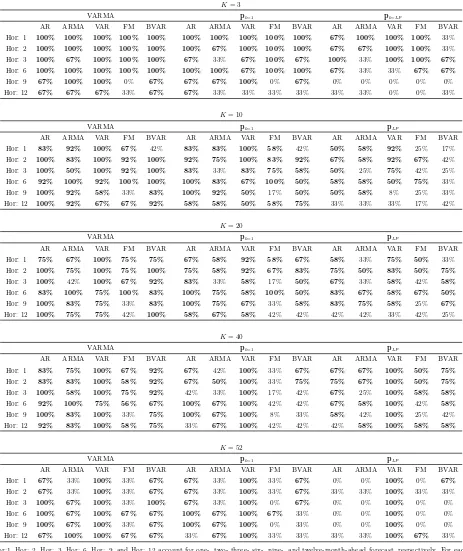
We organize the results as follows. Table 3 reports a summary of the forecast results
across the different datasets and presents, for each system size, three panels. The first
panel reports the frequency (in percentage points) for which at least one of the VARMA
specifications (pk=1, pk=2,pk=3,pk=4,pk=5,pk=6, pHK, and pLP) outperforms (delivers the
lowest RelMSFE measures) the assigned group of competitors in a given forecast horizon.24
Similarly, the second and third panel display the frequencies for which the most restricted,
pk=1, and general, pLP, specifications outperform the assigned group of competitors. We
consider five groups of competitors: AR, ARMA, VAR, FM, and BVAR. The AR group
collects the AR(1) specification; ARMA has the ARMA(1,1) specification estimated with
IOLS and MLE; VAR contains the VAR(p∗) model; FM gathers the different factor model
specifications, namely theF MSC andF MIC3; and the BVAR collects the three BVAR spec-ifications: BVARSC, BVAR0.2 and BVARopt. Finally, Table 4 compares the performance of
the IOLS estimator with the DJ2, HK, and KP estimators. We report the frequency (in
percentage points) for which the IOLS estimator outperforms the alternative estimators for
each forecast horizon. A comprehensive set of results is available in Section S.4.4 in the
online Supplement (Tables S.15 to S.28), making it possible to assess the forecast
perfor-mance of all VARMA specifications and the alternative model competitors in all datasets
and system sizes up to the level of the key macroeconomic variables. Convergence rates for
the IOLS estimator are also reported for all VARMA specifications. In what follows, we
draw from these tables when discussing the empirical results.
Starting with K = 3, we find that VARMA models largely outperform the AR, VAR, FM, and the BVAR groups up to the sixth-step-ahead forecast (see Table 3). Specifically,
thepk=1andpk=2specifications are the ones which deliver the best results. VARMA models
also outperform the ARMA(1,1) specifications, which reinforces the idea that modelling the
three key macroeconomic variables in a multivariate context pays off. Taking into account
all forecast horizons, VARMA models deliver the best forecast in 67% of the cases.
We now summarize the results for the medium and large datasets, (K = 10, K = 20, K = 40, and K = 52). We start by discussing the results for K = 10. For short horizons
24Percentages are computed across the three key macroeconomic variables and the four datasets discussed
(Hor:1 - Hor:6), VARMA models deliver the lowest RelMSFE in 63% of the cases.
Com-pared with the BVAR group, VARMA models remain dominant, delivering more accurate
forecasts in 81% of the cases (Hor:1 - Hor:6). Moreover, the pk=1 and pk=2 specifications
are the ones that usually deliver the lowest RelMSFE measures among the VARMA
speci-fications. Specifically,pk=1 minimizes the SC3 criterion in all datasets, which indicates that
choosing the Kronecker indices that minimize the SC3criterion pays off in terms of forecast
accuracy. Increasing the number of nonzero Kronecker indices from three to six,pk=3,pk=4,
pk=5, andpk=6specifications, delivers stable RelMSFE measures which are less often the best
among the competitors. This is in line with the large datasets literature, which documents
that imposing restrictions on the parameter matrices of a standard VAR model improves
forecast accuracy (De Mol, Giannone, and Reichlin (2008), Carriero, Kapetanios, and
Mar-cellino (2011), and Ba´nbura, Giannone, and Reichlin (2010)). Choosing the Kronecker
indices according to the general L¨utkepohl-Poskitt procedure and the Hannan-Kavalieris
algorithm typically yields more complex models (up to eight nonzero Kronecker indices),
stable RelMSFE measures, and a slightly less accurate forecast performance. Specifically,
while the pLP generally outperforms the AR, ARMA, and VAR for short horizons, it is
outperformed by FM, and BVAR specifications. With regard to the estimation of VARMA
models, the IOLS estimator works well, presenting an average convergence rate of 93%.
Additionally, its relative performance with respect to the DJ2, HK, and KP estimators is
positive. Considering thepk=1 and thepk=2 specifications, the IOLS estimator outperforms
its linear competitors in 81% of the cases (Table 4).
We now discuss the results for K = 20. Overall, VARMA models are very competitive in the short horizons (Hor:1 - Hor:6), outperforming the AR, ARMA, VAR, FM and BVAR
groups in 90%, 71%, 94%, 79%, and 88% of the cases, respectively. Results are also stable
across the different datasets and VARMA specifications, showing robustness of the VARMA
framework. Differently from the K = 10 scenario, there is not a clear winner among the VARMA specifications, although pk=1 remains very competitive and minimizes the
SC3 criterion. While setting the number of nonzero Kronecker indices as k∈ (2,3,4,5,6) typically does not improve forecast accuracy (pk=6 in Dataset 3 is the exception), the data
driven L¨utkepohl-Poskitt procedure emerges as a strong competitor and yields the most
accurate forecasts among all VARMA specifications in 29% of the cases. The IOLS estimator
more accurate forecasts than the DJ2, HK, and KP estimators in the long horizons. The
strong performance of the HK estimator in the short horizons is in line with the Monte
Carlo results.
Considering the case of large datasets (K= 40), we find that VARMA models stay very
competitive, outperforming the AR, ARMA, VAR, FM, and BVAR groups in 92%, 81%,
96%, 58%, and 82% of the cases, respectively. The general pLP specification now emerges
as the clear winner among the VARMA specifications, as it produces the most accurate
forecasts in 46% of the cases. In turn, the L¨utkepohl-Poskitt procedure is able to select the
relevant Kronecker indices to forecast the key macroeconomic variables and preserves some
degree of sparseness in the parameter matrices, which is important when forecasting using
rich datasets. The good performance of the pLP specification is also due to the use of the
IOLS estimator, as the IOLS estimator outperforms the DJ2, HK, and KP estimators in
68%, 71%, and 94% of the cases (Table 4). Indeed, the Monte Carlo simulations show that
the IOLS estimator delivers an outstanding performance in large sized systems, (K = 40
and K = 52). We report marginal gains in terms of forecast accuracy when moving from thepk=1 specification to the more general models where the number of nonzero Kronecker
indices are k ∈ (2,3,4,5,6). Similarly to the case of the pLP specification, the IOLS
estimator systematically delivers more accurate forecasts than the alternative estimators.
Considering the specifications withk∈(1,2,3,4,5,6), the IOLS estimator outperforms the DJ2, HK, and KP estimators in 79%, 87%, and 86% of the cases, respectively (Table 4),
and improves the RelMSFE measures in 19%, 33%, and 40% on average for the DJ2, HK,
and KP estimators, respectively (Hor:1 - Hor:6).25 Finally, the IOLS estimator remains a
robust alternative, achieving convergence in 93% of the rolling windows (all specifications).
We now turn our attention to the results using the entire dataset (K = 52). When
comparing the performance of VARMA models with the BVAR group, the former delivers
lower RelMSFE measures in 72% of the cases. This is a strong result in favour of VARMA
models, since BVAR specifications are known to be very competitive when forecasting with
large datasets. Overall, factor models deliver the best performance. Among the VARMA
specifications, pk=1 and pk=2 deliver the best results. Increasing the number of nonzero
Kronecker indices to k ∈ (3,4,5,6) delivers at most marginal improvements in terms of RelMSFE measures. When the IOLS estimator presents low convergence rates (pLP and
pHK specifications), VARMA models become less competitive. Alternatively, using the
RelMSFE measures obtained with the DJ2, HK, and KP estimators does not help either, as
they yield no qualitative improvement in terms of forecast hierarchy when compared to the
IOLS based measures. On the comparison of the IOLS and the alternative linear estimators,
the IOLS estimator largely outperforms (presents values greater than 50%) the DJ2, HK,
and KP estimators for thepk=1,pk=2,pk=3,pk=4,pk=5, andpk=6specifications. Specifically,
the IOLS estimator outperforms the DJ2, HK, and KP estimators in 83%, 98%, and 94%
of the cases, respectively (Table 4), and improves the RelMSFE measures compared to the
DJ2, HK, and KP estimators an average of 33%, 54%, and 70%, respectively, (Hor:1
-Hor:3).26 Finally, convergence rates for these specifications are 100%.
To sum up the results of this section, VARMA models estimated using the IOLS
estima-tor are generally very competitive and able to beat the four most prominent competiestima-tors in
this type of study: AR, ARMA, factor models and BVAR models. This finding is especially
present for thepk=1andpLP specifications. VARMA results are also stable across the
differ-ent datasets and Kronecker indices specifications, indicating that the framework adopted is
fairly robust. Considering all system sizes and datasets, VARMA specifications deliver the
lowest RelMSFE measures for the one-, two-, three-, and six-month-ahead forecast in 63%
of the cases, indicating that VARMA models are indeed strong candidates to forecast key
macroeconomic variables using small, medium and large sized datasets. It is particularly
relevant to highlight the performance of VARMA models relative to the BVAR models, as
VARMA models systematically deliver more accurate forecasts for all datasets. The IOLS
estimator is a valid alternative to deal with large and complex VARMA systems
(conver-gence rates averaging 92%) and compares favourably with the main linear competitors (more
accurate forecasts in 69% of the cases). Finally, our findings reinforce two important aspects:
using the Echelon form transformation either in the fashion of DGPs III-VI or using the
L¨utkepohl-Poskitt procedure is a powerful tool to deal with high-dimensional models; and
that IOLS estimator is particularly suitable to estimate high-dimensional VARMA models,
as the Monte Carlo simulations and empirical results suggest.