Munich Personal RePEc Archive
Quasi maximum likelihood estimation for
simultaneous spatial autoregressive
models
Wang, Luya and Li, Kunpeng and Wang, Zhengwei
November 2014
Online at
https://mpra.ub.uni-muenchen.de/59901/
Quasi maximum likelihood estimation for simultaneous
spatial autoregressive models
Luya Wang∗ and Kunpeng Li† and Zhengwei Wang‡
Abstract
This paper considers the problem of estimating a simultaneous spatial autoregrsive model (SSAR). We propose using the quasi maximum likelihood method to es-timate the model. The asymptotic properties of the maximum likelihood estimator including consistency and limiting distribution are investigated. We also run Monte Carlo simulations to examine the finite sample performance of the maximum likelihood estimator.
Key Words: Simultaneous equations model, Spatial autoregressive model, Maxi-mum likelihood estimation, Asymptotic theory.
∗
The corresponding author. School of Banking and Finance, University of International Business and Economics, Beijing, China, 100029, Email:[email protected]
†School of International Economics and Management, Capital University of Economics and Business,
Beijing, China,
1
Introduction
Spatial econometric models provide an effective way to study the spatial interactions among units and are widely used in urban, real estate, regional, public, agricultural, environmental economics. Among the spatial models, spatial autoregressive (SAR) model proposed by Cliff and Ord (1973) has received much attention. Popular methods to estimate SAR models include the maximum likelihood method (Anselin, 1988; Lee, 2004; Baltagi and Bresson, 2011) and the generalized moments method (Kelejian and Prucha, 1998; Kelejian and Prucha, 1999; Baltagi and Liu, 2011). Readers are referred to Lee and Yu (2010) for a survey on a recent development of spatial models.
The spatial econometric literature, so far, focuses mainly on the single equation SAR model. In structural economic models, the endogenous variables, which possibly have spatial effects, are simultaneously determined in equilibrium. As a result, a single equation model may not be appropriate to estimate the structural parameters. This motivates the necessity to extend the single equation model to a multiple equation system. In this paper, we study the estimation and inferential theory of a simultaneous spatial autoregressive (SSAR) model. We establish the asymptotic theory of the maximum likelihood estimator including consistency and limiting distribution, which is new to the spatial econometric literature.
A related work to our paper is Baltagi and Deng (2012) who consider estimating a SSAR model in a random effects panel data framework. They propose a three-stage least squares method to estimate the coefficients, but they do not study the asymptotic properties of the estimator. In this paper we use the quasi maximum likelihood method to estimate a SSAR model under cross-sectional data setup. Although we focus on the cross-sectional data, the result of this paper, with extra efforts, can be extended to deal with a fixed effects panel data model. This would complement Baltagi and Deng’s work.
The rest of the paper is organized as follows. Section 2 describes the model and lists the assumptions that are needed for the asymptotic analysis. Section 3 presents the quasi likelihood function and the asymptotic theory of the MLE. Section 4 conducts Monte Carlo simulations to investigate the finite sample performance of the MLE. Section 5 concludes the paper. In appendix A, we give a detailed expressions for two matrices that are im-portant parts of the limiting variance. The technical materials including the proofs of the main results of the paper are delegated to the supplementary appendix B.
2
Model and Assumptions
We consider the following SSAR model
Y1 =ρ1W1Y1+γ1Y2+X1β1+e1 (1)
Y2 =ρ2W2Y2+γ2Y1+X2β2+e2 (2)
where Y1 and Y2 are both N ×1 dependent variables. W1 and W2 are respective N ×
N spatial weights matrices. X1 is a set of N ×k1 explanatory variables and β1 is the
corresponding k1-dimensional vector of coefficients. X2 is a set of N ×k2 explanatory
In the SSAR model (1) and (2), we consider a simple case of two equations system. We note that this is just for expositional simplicity. Extension to more equations system involves no fundamentally new contents.
The SSAR model can be rewritten as
"
IN −ρ1W1 −γ1IN
−γ2IN IN −ρ2W2
#
| {z }
≡S(ρ1,ρ2,γ1,γ2)
" Y1
Y2
#
| {z }
≡Y
=
" X1 0
0 X2
#
| {z }
≡X
" β1
β2
#
| {z }
≡β
+
" e1
e2
#
| {z }
≡e
. (3)
Letδ= (ρ1, ρ2, γ1, γ2), the above model is equivalent to
S(δ)Y =Xβ+e, (4)
whereY, X, β andeare defined in (3). Throughout the paper, we use the symbols with as-terisk to denote the underlying true values, for example,ρ∗1,γ1∗, etc. Letδ∗ = (ρ∗1, ρ∗2, γ1∗, γ2∗). We make the following assumptions for the subsequent analysis.
Assumption A:Lete1i ande2i be the disturbances of the two equations
correspond-ing to the ith observation. We assume that e1i and e2i are mutually independent with
E(e4+1i κ) ≤C and E(e4+2i κ) ≤C for some given κ, where C is a generic positive constant. In addition e1i and e2i are both independent and identically distributed over i with the
variancesσ2
1 and σ22, respectively.
Assumption B:MatrixS(δ) is invertible for all δ∈∆, where ∆ is a compact set, and
δ∗ is an interior point of ∆.
Assumption C: W1 and W2 are N ×N exogenously spatial weights matrices such
that the diagonal elements of W1 and W2 are all zeros. In addition, both W1 and W2 are
bounded in absolute value in column and row sums. Furthermore, S−1(δ) is bounded in
absolute value in column and row sums uniformly inδ∈∆.
Assumption D:The elements ofX are nonrandom and bounded in absolute value by some constantC. In addition,Q= lim
N→∞
1
NX′X exists and is positively definite.
Assumption E:One of the following two conditions holds: E1 For any δ6=δ∗, lim
N→∞[(P−P
∗)S−1(δ∗)Xβ∗, X]′[(P−P∗)S−1(δ∗)Xβ∗, X]/N is posi-tively definite, where
P =
"
ρ1W1 γ1IN
γ2IN ρ2W2
#
, P∗ =
"
ρ∗1W1 γ1∗IN
γ2∗IN ρ∗2W2
# .
E2 Let R(δ) =S(δ)′S−1′(δ∗)Σ∗eeS−1(δ∗)S(δ) where Σ∗ee = var(e) = diag(σ1∗2IN, σ2∗2IN),
andR11(δ) andR22(δ) be the respective left-upper and right-lowerN×N submatrices
ofR(δ). Then for any δ6=δ∗,
lim inf
N→∞
ln
1
Ntr[R11(δ)] + ln
1
Ntr[R22(δ)] −
1
N ln R(δ)
>0.
variables and the underlying parameters. These conditions are standard in the spatial econometric models. Similar assumptions are also made in Yu et al. (2008). Assumption D assumes that the explanatory variables are nonrandom. If the explanatory variable is random but independent with the disturbance, then the analysis of this paper can be viewed as conditional on the realizations of explanatory variables. Assumption E is the identification for the parametersδ. Assumption E1 is a local identification condition since it depends on the underlying valueβ∗. If β∗= 0, Assumption E1 breaks down. To account for this possibility, we need a stronger condition. This gives Assumption E2, which is a global identification that does not depend on β∗. Assumptions E1 and E2 correspond to Assumptions 8 and 9 in Lee (2004), respectively. But our conditions are more complicated. This is because the transformation matrixS(δ) has a more complicated form and the errors in (4) are not homoscedastic.
3
Likelihood function and asymptotic theory
Suppose thate1i and e2i are normally distributed. Therefore the log-likelihood function is
L(θ) =− 1
2N ln|Σee|+
1
N ln|S(δ)| −
1
2N[S(δ)Y −Xβ]
′Σ−1
ee[S(δ)Y −Xβ] (5)
where Σee = diag(σ21IN, σ22IN) and θ = (δ, β1, β2, σ12, σ22). Let Θ be the parameters space
that are specified by Assumptions B and C. The quasi maximum likelihood estimator (MLE) is defined as
ˆ
θ= argmax
θ∈Θ L
(θ).
The following theorem delivers the limiting distribution of the MLE. The consistency and the rate of convergence are implicitly given by the theorem.
Theorem 1 Under Assumptions A-E, when N → ∞,
√
N(ˆθ−θ∗)−→d N(0,Ω⋆−1(Ω⋆+ Σ⋆)Ω⋆−1).
withΩ⋆= lim
N→∞ΩandΣ
⋆= lim
N→∞Σ, whereΩandΣare defined by (6) and (7) in Appendix. The above theorem shows that the limiting variance of the MLE has a sandwich expres-sion. This is a well-known result in Quasi-MLE (see Lee (2004)), due to the misspecification of the distribution of the errors. However, if the errors are normally distributed, the dis-tribution of errors is correctly specified. Then the limiting variance has a more elegant expression, which is stated in the following theorem.
Theorem 2 Under the assumptions of Theorem 1, ife1i ande2i are normally distributed,
when N → ∞, we have √
N(ˆθ−θ∗)→−d N(0,Ω⋆−1).
Theorem 2 follows from Theorem 1 directly by noting that Σ⋆ = 0 whene1i and e2iare
4
Monte Carlo simulations
We run the Monte Carlo simulations to investigate the finite sample performance of the MLE. The data are generated according to
Y1 =α1+ρ1W1Y1+γ1Y2+x1ζ1+e1
Y2 =α2+ρ2W2Y2+γ2Y1+x2ζ2+e2
withα1 = 1, α2 = 1,ρ1 = 0.3,ρ2 = 0.4,γ1 = 0.2, γ2 = 0.4, ζ1 = 1, ζ2 = 2, σ12 = 0.5 and
σ2
2 = 2. Let β1 = (α1, ζ1)′, β2 = (α2, ζ2)′,X1 = (1N, x1) and X2 = (1N, x2) where1N is a
N-dimensional vector with all elements equal to 1. Then we have the same expressions as model (1) and (2). As for the spatial weights matrices,W1 is fixed to be
one-ahead-and-one-behind weights matrix and W2 is fixed to be three-ahead-and-three-behind weights
matrix. The “q ahead and q behind” spatial weights matrix is defined the same as in Kelejian and Prucha (1999) and Kapoor et al. (2007). More specifically, all the units are arranged in a circle and each unit is affected only by the q units immediately before it and immediately after it with equal weight. Following Kelejian and Prucha (1999), we normalize the spatial weights matrix by letting the sum of each row be equal to 1 (so the weight is 21q). The spatial weights matrix generated in this way is called “q ahead and
q behind”. The other terms such as x1i, x2i, e1i and e2i are all generated independently
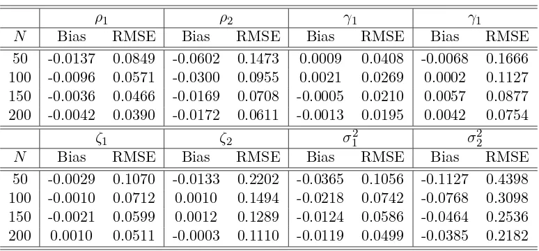
[image:6.612.113.500.436.616.2]from N(0,1). The following table presents the performance of the MLE under different sample size, which are obtained by 1000 repetitions. From the table, we see that the MLE performs well in our simulations.
Table 1: The performance of the MLE
ρ1 ρ2 γ1 γ1
N Bias RMSE Bias RMSE Bias RMSE Bias RMSE 50 -0.0137 0.0849 -0.0602 0.1473 0.0009 0.0408 -0.0068 0.1666 100 -0.0096 0.0571 -0.0300 0.0955 0.0021 0.0269 0.0002 0.1127 150 -0.0036 0.0466 -0.0169 0.0708 -0.0005 0.0210 0.0057 0.0877 200 -0.0042 0.0390 -0.0172 0.0611 -0.0013 0.0195 0.0042 0.0754
ζ1 ζ2 σ12 σ22
N Bias RMSE Bias RMSE Bias RMSE Bias RMSE 50 -0.0029 0.1070 -0.0133 0.2202 -0.0365 0.1056 -0.1127 0.4398 100 -0.0010 0.0712 0.0010 0.1494 -0.0218 0.0742 -0.0768 0.3098 150 -0.0021 0.0599 0.0012 0.1289 -0.0124 0.0586 -0.0464 0.2536 200 0.0010 0.0511 -0.0003 0.1110 -0.0119 0.0499 -0.0385 0.2182
5
Conclusion
Appendix A: The expressions of
Ω
and
Σ
In this appendix, we give the explicit expressions of Ω and Σ. The matrix Ω is defined as
Ω =
Ω11 Ω12 Ω13 Ω14 Ω15 0 Ω17 0
∗ Ω22 Ω23 Ω24 0 Ω26 0 Ω28
∗ ∗ Ω33 Ω34 Ω35 0 Ω37 0
∗ ∗ ∗ Ω44 0 Ω46 0 Ω48
∗ ∗ ∗ ∗ Ω55 0 0 0
∗ ∗ ∗ ∗ ∗ Ω66 0 0
∗ ∗ ∗ ∗ ∗ ∗ 2σ1∗4
1 0
∗ ∗ ∗ ∗ ∗ ∗ ∗ 1
2σ∗4 2
(6)
with
Ω11=
1
N σ∗2 1
h
(V11∗X1β1∗+V12∗X2β2∗)′W1′W1(V11∗X1β1∗+V12∗X2β2∗) +σ1∗2tr(W1V11∗W1V11∗)
+σ∗12tr(V11∗′W1′W1V11∗) +σ2∗2tr(V12∗′W1′W1V12∗)
i ,
Ω12=
1
Ntr(W1V
∗
12W2V21∗),
Ω13=
1
N σ∗12 h
(V11∗X1β1∗+V12∗X2β2∗)′W1′(V21∗X1β1∗+V22∗X2β2∗) +σ∗12tr(W1V11∗V21∗)
+σ∗12tr(V21∗′W1V11∗) +σ2∗2tr(V22∗′W1V12∗)
i ,
Ω14=
1
Ntr(V
∗
12V11∗W1),
Ω15=
1
N σ∗12(V
∗
11X1β1∗+V12∗X2β2∗)′W1′X1,
Ω17= 1
N σ∗2 1
tr(W1V11∗),
Ω22=
1
N σ∗2 2
h
(V21∗X1β1∗+V22∗X2β2∗)′W2′W2(V21∗X1β1∗+V22∗X2β2∗) +σ2∗2tr(W2V22∗W2V22∗)
+σ∗22tr(V22∗′W2′W2V22∗) +σ1∗2tr(V21∗′W2′W2V21∗)
i ,
Ω23=
1
Ntr(W2V
∗
21V22∗),
Ω24=
1
N σ∗2 2
h
(V21∗X1β1∗+V22∗X2β2∗)′W2′(V11∗X1β1∗+V12∗X2β2∗)
+σ∗22tr(W2V22∗V12∗) +σ2∗2tr(V12∗′W2V22∗) +σ1∗2tr(V11∗′W2V21∗)
i ,
Ω26=
1
N σ∗2 2
(V21∗X1β1∗+V22∗X2β2∗)′W2′X1,
Ω28= 1
N σ∗2 2
tr(W2V22∗),
Ω33=
1
N σ∗2 1
h
+σ∗12tr(V21∗′V21∗) +σ2∗2tr(V22∗′V22∗),
Ω34= 1
Ntr(V
∗
11V22∗),
Ω35=
1
N σ∗12(V
∗
21X1β1∗+V22∗X2β2∗)′X1,
Ω37=
1
N σ∗12tr(V
∗
21),
Ω44=
1
N σ∗2 2
h
(V11∗X1β1∗+V12∗X2β2∗)′(V11∗X1β1∗+V12∗X2β∗2)′+σ2∗2tr(V12∗V12∗)
+σ∗22tr(V12∗′V12∗) +σ1∗2tr(V11∗′V11∗),
Ω46=
1
N σ∗22(V
∗
11X1β1∗+V12∗X2β2∗)′X2,
Ω48=
1
N σ∗22tr(V
∗
12),
Ω55=
1
N σ∗2 1
X1′X1,
Ω66= 1
N σ∗2 2
X2′X2,
and the matrix Σ is defined as
Σ =
Σ11 0 Σ13 0 Σ15 0 Σ17 0
∗ Σ22 0 Σ24 0 Σ26 0 Σ28
∗ ∗ Σ33 0 Σ35 0 Σ37 0
∗ ∗ ∗ Σ44 0 Σ46 0 Σ48
∗ ∗ ∗ ∗ 0 0 Σ57 0
∗ ∗ ∗ ∗ ∗ 0 0 Σ68
∗ ∗ ∗ ∗ ∗ ∗ Σ77 0
∗ ∗ ∗ ∗ ∗ ∗ ∗ Σ88
(7) with
Σ11=
2κ3
N σ∗4 1
N
X
i=1
W1,i∗V11∗,∗iW1,i∗(V11∗X1β1∗+V12∗X2β2∗) +
κ4−3σ1∗4
N σ∗4 1
tr[(W1V11∗)◦(W1V11∗)],
Σ13=
1
N σ1∗4 n
κ3
N
X
i=1
W1,i∗
h
(V11∗X1β1∗+V12∗X2β∗2)V21∗,ii+V11∗,∗i(V21∗,i∗X1β1∗+V22∗,i∗X2β2∗)
i
+ (κ4−3σ1∗4)tr[(W1V11∗)◦V21∗]
o ,
Σ15=
κ3
N σ1∗4
N
X
i=1
W1,i∗V11∗,∗iX1,i,
Σ17=
1 2N σ∗6
1 h κ3 N X i=1
W1,i∗(V11∗X1β1∗+V12∗X2β2∗) + (κ4−3σ1∗4)tr(W1V11∗)
i ,
Σ22=
2µ3
N σ2∗4
N
X
i=1
W2,i∗V22∗,∗iW2,i∗(V21∗X1β1∗+V22∗X2β2∗) +
µ4−3σ∗24
N σ2∗4 tr[(W2V
∗
Σ24=
1
N σ2∗4 n
µ3
N
X
i=1
W2,i∗
h
(V21∗X1β1∗+V22∗X2β2∗)V12∗,ii+V22∗,∗i(V11∗,i∗X1β1∗+V12∗,i∗X2β2∗)
i
+ (µ4−3σ∗24)tr[(W2V22∗)◦V12∗]
o ,
Σ26=
µ3
N σ2∗4
N
X
i=1
W2,i∗V22∗,∗iX2,i,
Σ28= 1
2N σ∗6 2
h µ3
N
X
i=1
W2,i∗(V21∗X1β1∗+V22∗X2β2∗) + (µ4−3σ2∗4)tr(W2V22∗)
i ,
Σ33=
1
N σ∗4 1
h
2κ3
N
X
i=1
(V21∗,i∗X1β∗1+V22∗,i∗X2β2∗)V21∗,ii+ (κ4−3σ1∗4)tr(V21∗ ◦V21∗)
i ,
Σ35= 1
N σ∗4 1
κ3
N
X
i=1
V21∗,iiX1,i,
Σ37=
1 2N σ∗6
1
h κ3
N
X
i=1
(V21∗,i∗X1β∗1+V22∗,i∗X2β2∗) + (κ4−3σ1∗4)tr(V21∗)
i ,
Σ44=
1
N σ2∗4 h
2µ3
N
X
i=1
(V11∗,i∗X1β1∗+V12∗,i∗X2β2∗)V12∗,ii+ (µ4−3σ2∗4)tr(V12∗ ◦V12∗)
i ,
Σ46=
1
N σ∗4 2
µ3
N
X
i=1
V12∗,iiX2,i,
Σ48=
1 2N σ2∗6
h µ3
N
X
i=1
(V11∗,i∗X1β1∗+V12∗,i∗X2β2∗) + (µ4−3σ2∗4)tr(V12∗)
i ,
Σ57= 1
2N σ∗6 1
κ3
N
X
i=1
X1,i,
Σ68=
1 2N σ∗6
2
µ3
N
X
i=1
X2,i,
Σ77=
1
4σ∗18(κ4−3σ
∗4 1 ),
Σ88=
1
4σ∗28(µ4−3σ
∗4 2 ),
The symbols appearing in the above expression are defined as follows: κ3 =E(e31i), µ3 =
E(e3
2i), κ4 =E(e41i) andµ4 =E(e42i); V∗ =S−1(δ∗) and V11∗, V12∗, V21∗, V22∗ are defined by
V∗ =
"
V11∗ V12∗ V21∗ V22∗ #
.
Mi∗ denotes the ith row of M; M∗i denotes the ith column of M and Mij denotes the
References
Anselin, L. (1988). Spatial econometrics: methods and models. The Netherlands: Kluwer Academic Publishers.
Baltagi, B. H. and Deng, Y. (2012). EC3SLS estimator for a simultaneous system of spatial autoregressive equations with random effects. Econometric Review, Forthcoming.
Baltagi, B. H. and Bresson, G. (2011). Maximum likelihood estimation and lagrange mul-tiplier tests for panel seemingly unrelated regressions with spatial lag and spatial errors: an application to hedonic housing prices in Paris, Journal of Urban Economics, 69(1), 24-42.
Baltagi, B. H. and Liu, L. (2011). An improved generalized moments estimator for a spatial moving average error model,Economics Letters, 282-284.
Cliff, A. D., and Ord, J. K. (1973) Spatial autocorrelation, London: Pion Ltd.
Kapoor, M., Kelejian, H. H., and Prucha, I. R. (2007). Panel data models with spatially correlated error components.Journal of Econometrics, 140(1), 97-130.
Kelejian, H. H., and Prucha, I. R. (1998) A generalized spatial two-stage least squares procedure for estimating a spatial autoregressive model with autoregressive disturbances.
The Journal of Real Estate Finance and Economics, 17(1), 99-121.
Kelejian, H. H., and Prucha, I. R. (1999) A generalized moments estimator for the autore-gressive parameter in a spatial model.International economic review, 40(2), 509-533.
Lee, L. (2004) Asymptotic distribution of quasi-maximum likelihood estimators for spatial augoregressive models,Econometrica, 72(6), 1899–1925.
Lee L., and Yu J. (2010). Some recent developments in spatial panel data models.Regional Science and Urban Economics, 40(5), 255–271.
Supplementary Appendix B: Quasi maximum likelihood
es-timation for simultaneous spatial autoregressive models
In this supplementary Appendix B, we provide a detailed proof for Theorem 1. Consider the following likelihood function
L(θ) = −1 2lnσ
2 1−
1 2lnσ
2 2+
1
N ln|S(δ)| −
1
2N[S(δ)Y −Xβ]
′Σ−1
ee[S(δ)Y −Xβ]
+1 2lnσ
∗2 1 +
1 2lnσ
∗2 2 −
1
N ln|S(δ
∗) |+ 1
whereθ= (δ, β1′, β2′, σ21, σ22)′. The above objective function is only different from the original likelihood function with a constant and will be treated as the objective function in the subsequent analysis. Givenδ, σ12, σ22, it is seen that the objective function is maximized at
β1⋆(δ) = (X1′X1)−1X1′(Y1−ρ1W1Y1−γ1Y2), (S.1)
β2⋆(δ) = (X2′X2)−1X2′(Y2−ρ2W2Y2−γ2Y1). (S.2)
Using the above two equations to concentrate outβ1 and β2, the objective function is
L(θ) = −1 2lnσ
2 1−
1 2lnσ
2 2+
1
N ln|S(δ)|
− 1
2N σ21(Y1−ρ1W1Y1−γ1Y2)
′M
X1(Y1−ρ1W1Y1−γ1Y2)
− 1 2N σ2
2
(Y2−ρ2W2Y2−γ2Y1)′MX2(Y2−ρ2W2Y2−γ2Y1)
+1 2lnσ
∗2 1 +
1 2lnσ
∗2 2 −
1
N ln|S(δ
∗)|+ 1
Again, givenρ1, ρ2, γ1, γ2, it is seen that the above objective function is optimized
σ1⋆2(δ) = 1
N(Y1−ρ1W1Y1−γ1Y2)
′M
X1(Y1−ρ1W1Y1−γ1Y2), (S.3)
σ2⋆2(δ) = 1
N(Y2−ρ2W2Y2−γ2Y1)
′M
X2(Y2−ρ2W2Y2−γ2Y1). (S.4)
Using the preceding two solutions to further concentrate out σ21 and σ22, the objective function now is
L(δ) =−1 2lnσ
⋆2 1 (δ)−
1 2lnσ
⋆2 2 (δ) +
1
N ln|S(δ)|+
1 2lnσ
∗2 1 +
1 2lnσ
∗2 2 −
1
N ln|S(δ
∗)|.
Hereafter, we use S∗ to represent S(δ∗) for notational simplicity. Let
P =
"
ρ1W1 γ1IN
γ2IN ρ2W2
#
, P∗ =
"
ρ∗1W1 γ1∗IN
γ2∗IN ρ∗2W2
# .
By the definition, we have
"
Y1−ρ1W1Y1−γ1Y2
Y2−ρ2W2Y2−γ2Y1
#
Let V∗ = S∗−1 and R(δ) = S(δ)S∗−1Σ∗
eeS∗−1′S(δ)′. For ease of exposition, we partition
R(δ) andV∗ into
R(δ) =
"
R11(δ) R12(δ)
R21(δ) R22(δ)
#
, V∗=
"
V11∗ V12∗ V21∗ V22∗ #
.
Then we have
Y1−ρ1W1Y1−γ1Y2 =X1β1∗+e1−
h
(ρ1−ρ∗1)W1V11∗ + (γ1−γ1∗)V21∗
i
(X1β1∗+e1)
−h(ρ1−ρ∗1)W1V12∗ + (γ1−γ1∗)V22∗
i
(X2β2∗+e2) (S.5)
Y2−ρ2W2Y2−γ2Y1 =X2β2∗+e2−
h
(ρ2−ρ∗2)W2V21∗ + (γ2−γ2∗)V11∗
i
(X1β1∗+e1)
−h(ρ2−ρ∗2)W2V22∗ + (γ2−γ2∗)V12∗
i
(X2β2∗+e2) (S.6)
Using the above results, we can further rewrite the objective function as
L(δ) =L1(δ) +L2(δ),
with
L1(δ) =−
1 2ln
W1(δ) +
1
Ntr[R11(δ)] − 1 2ln
W1(δ) +
1
Ntr[R11(δ)] +
1
2N ln|R(δ)|
and
L2(δ) = ln
W1(δ) +
1
Ntr[R11(δ)] +R1(δ) −ln
W1(δ) +
1
Ntr[R11(δ)]
+ ln
W2(δ) +
1
Ntr[R22(δ)] +R2(δ) −ln
W1(δ) +
1
Ntr[R22(δ)] ,
where
W1(δ) =
1
NU1(δ)
′M
X1U1(δ), W2(δ) =
1
NU2(δ)
′M
X2U2(δ).
In addition,
R1(δ) =
2
NU1(δ)
′M
X1U3(δ)e1−
2
NU1(δ)
′M
X1U5(δ)e2−
2
Ne
′
1U3(δ)′MX1U5(δ)e2
−N1 e′1U3(δ)′PX1U3(δ)e1+
1
Ntr h
U3(δ)′U3(δ)(e1e′1−σ∗12IN)
i
−1
Ne
′
2U5(δ)′PX1U5(δ)e2+
1
Ntr h
U5(δ)′U5(δ)(e2e′2−σ2∗2IN)
i ,
and
R2 =
2
NU2(δ)
′M
X2U4(δ)e2−
2
NU2(δ)
′M
X2U6(δ)e1−
2
Ne
′
1U6(δ)′MX2U4(δ)e2
−1
Ne
′
2U4(δ)′PX2U4(δ)e2+
1
Ntr h
U4(δ)′U4(δ)(e2e′2−σ∗22IN)
i
−N1 e′1U6(δ)′PX2U6(δ)e1+
1
Ntr h
U6(δ)′U6(δ)(e1e′1−σ1∗2IN)
i .
U1(δ) = (ρ1−ρ∗1)W1(V11∗X1β1∗+V12∗X2β∗2) + (γ1−γ1∗)(V21∗X1β1∗+V22∗X2β2∗),
U2(δ) = (ρ2−ρ∗2)W2(V21∗X1β1∗+V22∗X2β∗2) + (γ2−γ2∗)(V11∗X1β1∗+V12∗X2β2∗),
U3(δ) =IN −(ρ1−ρ∗1)W1V11∗ −(γ1−γ1∗)V21∗,
U4(δ) =IN −(ρ2−ρ∗2)W2V22∗ −(γ2−γ2∗)V12∗,
U5(δ) = (ρ1−ρ∗1)W1V12∗ + (γ1−γ1∗)V22∗,
U6(δ) = (ρ2−ρ∗2)W2V21∗ + (γ2−γ2∗)V11∗.
Under Assumptions A-D, it can be shown that |R1(δ)|= op(1) and |R2(δ)|= op(1)
uni-formly on Θ. These two results imply
sup
θ∈Θ|L
(δ)− L1(δ)|=op(1). (S.7)
To show the consistency, it suffices to show
sup
θ∈Nc ǫ
(L1(δ)− L1(δ∗))<0.
where Nc
ǫ denotes the complement of an open neighborhood of δ
∗ in ∆ of diameter of
ǫ. Our normalized objective function gives L1(δ∗) = 0. As regards to L1(δ), which is
equivalent to
L1(δ) =−
1 2
h
ln
1
Ntr[R11(δ)] −
1
N ln|R11(δ)| i
− 1 2
h
ln
1
Ntr[R22(δ)] −
1
N ln|R22(δ)| i
−12hlnW1(δ) +
1
Ntr[R11(δ)]
−ln1
Ntr[R11(δ)] i
−1 2
h
lnW2(δ) +
1
Ntr[R22(δ)]
−ln1
Ntr[R22(δ)] i
+ 1 2N ln
IN −R−221/2(δ)R21(δ)R11−1(δ)R12(δ)R−221/2(δ)
.
The first two terms are non-positive by the Jensen’s inequality. The third and fourth terms are also non-positive since W1(δ) and W2(δ) are non-negative for all δ. The last term is
also negative since all the eigenvalues ofIN−R−221/2(δ)R21(δ)R11−1(δ)R12(δ)R−221/2(δ) are no
greater than 1. Given these results, we have
L1(δ)≤0.
So we only need to show that for any pointδ 6=δ∗ and δ ∈∆ such that L1(δ)<0.
Notice that
W1(δ) +W2(δ) =
1
Nβ
∗′X′S∗−1(P−P∗)′M
X(P −P∗)S∗−1Xβ∗.
By Assumption E1, for anyδ6=δ∗, the above term is strictly greater than 0. This implies that either W1(δ) or W2(δ) or both W1(δ) and W2(δ) are greater than 0, which further
imply L1(δ)<0. Also notice that the expression
−1 2
h
ln
1
Ntr[R11(δ)] −
1
N ln|R11(δ)| i
−1 2
h
ln
1
Ntr[R22(δ)] −
1
+ 1 2N ln
IN −R−221/2(δ)R21(δ)R11−1(δ)R12(δ)R−221/2(δ)
is equivalent to
−1 2 h ln 1
Ntr[R11(δ)] + ln 1
Ntr[R22(δ)] i
+ 1
2N ln|R(δ)|.
If Assumption E2 holds, i.e., for anyδ6=δ∗,
ln
1
Ntr[R11(δ)] + ln 1
Ntr[R22(δ)] −
1
N ln|R(δ)| 6= 0,
we immediately obtain thatL1(δ)<0.
Now we show thatL1(δ) can identifyδ∗. This result, together with the uniform
conver-gence result (S.7), gives the consistency of ˆδ. Given the consistency of ˆδ, by (S.1)-(S.4) and Assumption D, we obtain the consistency of ˆβ1,βˆ2,σˆ12 and ˆσ22. This completes the proof of
consistency.
Given the consistency, we now derive the limiting distribution. By the definition of ˆθ, we have ∂L∂θ(ˆθ) = 0. By the Taylor expansion, it follows
0 = ∂L(ˆθ)
∂θ =
∂L(θ∗)
∂θ +
∂2L(˜θ)
∂θ∂θ′ (ˆθ−θ ∗),
where ˜θ is some point between ˆθ andθ∗. The above result implies
ˆ
θ−θ∗ =−h∂
2L(˜θ)
∂θ∂θ′
i−1h∂L(θ∗) ∂θ
i .
The first order conditions forρ1, ρ2, γ1, γ2, β1, β2, σ12 and σ22 are
∂L ∂ρ1 = 1 N h 1 σ2 1
(Y1−ρ1W1Y1−γ1Y2−X1β1)′W1Y1−tr[S−1(δ)A1]
i ∂L ∂ρ2 = 1 N h 1 σ2 2
(Y2−ρ2W2Y2−γ2Y2−X2β2)′W2Y2−tr[S−1(δ)A2]
i ∂L ∂γ1 = 1 N h 1 σ2 1
(Y1−ρ1W1Y1−γ1Y2−X1β1)′Y2−tr[S−1(δ)A3]
i ∂L ∂γ2 = 1 N h 1
σ22(Y2−ρ2W2Y2−γ2Y2−X2β2)
′Y
1−tr[S−1(δ)A4]
i
∂L ∂β1
= 1
N σ2 1
X1′(Y1−ρ1W1Y1−γ1Y2−X1β1)
∂L
∂β2
= 1
N σ2 2
X2′(Y2−ρ2W2Y2−γ2Y1−X2β2)
∂L
∂σ2 1
= 1 2N σ4
1
h
(Y1−ρ1W1Y1−γ1Y2−X1β1)′(Y1−ρ1W1Y1−γ1Y2−X1β1)−N σ12
i
∂L ∂σ22 =
1 2N σ14
h
(Y2−ρ2W2Y2−γ2Y1−X2β2)′(Y2−ρ2W2Y2−γ2Y1−X2β2)−N σ22
i
Notice that
implying
Y1=V11∗X1β∗1+V12∗X2β2∗+V11∗e1+V12∗e2 (S.8)
Y2=V21∗X1β∗1+V22∗X2β2∗+V21∗e1+V22∗e2 (S.9)
Given the above results, we have
∂L(θ∗)
∂θ =
1
N
[e′1W1(V11∗X1β1∗+V12∗X2β2∗) +e′1W1V11∗e1−σ∗12tr(W1V11∗) +e′1W1V12∗e2]/σ1∗2
[e′2W2(V21∗X1β1∗+V22∗X2β2∗) +e′2W2V21∗e1+e′2W2V22∗e2−σ∗22tr(W2V22∗)]/σ2∗2
[e′1V21∗X1β∗1+e′1V22∗X2β2∗+e′1V21∗e1−σ∗12tr(V21∗) +e′1V22∗e2]/σ∗12
[e′2V11∗X1β∗1+e′2V12∗X2β2∗+e′2V11∗e1+e′2V12∗e2−σ2∗2tr(V12∗)]/σ∗22
X1′e1/σ1∗2
X2′e2/σ2∗2
(e′1e1−N σ1∗2)/(2σ∗14)
(e′2e2−N σ2∗2)/(2σ∗24)
With the existence of high-order moments of e1i and e2i in Assumption 1, we can apply
the central limit theorem for linear-quadratic forms of Kelejian and Prucha (2001) to the above expression. This gives
√
N∂L(θ
∗)
∂θ
d
−
→N(0,Ω⋆+ Σ⋆). (S.10)
where Ω⋆ and Σ⋆ are defined in Theorem 1.
We proceed to consider the second order derivatives. By some tedious but straightfor-ward computation, we have
∂2L ∂ρ1∂ρ1
=−1
N
tr[S−1(δ)A1S−1(δ)A1] +Y′A′1A1Y /σ21
,
∂2L ∂ρ1∂ρ2
=−1
Ntr[S
−1(δ)A
2S−1(δ)A1],
∂2L
∂ρ1∂γ1
=−1
N
tr[S(δ)−1A3S(δ)−1A1] +Y′A′3A1Y /σ21
,
∂2L
∂ρ1∂γ2
=−1
Ntr[S
−1(δ)A
4S−1(δ)A1],
∂2L
∂ρ1∂β1
=− 1
N σ12X
′
1W1Y1,
∂2L
∂ρ1∂β2
= 0,
∂2L ∂ρ1∂σ12
=− 1
N σ4 1
(Y1−ρ1W1Y1−γ1Y2−X1β1)′W1Y1,
∂2L
∂ρ1∂σ22
= 0,
∂2L ∂ρ2∂ρ2
=−1
N
tr[S−1(δ)A2S−1(δ)A2] +Y′W2′W2Y
∂2L
∂ρ2∂γ1
=−1
Ntr[S
−1(δ)A
3S−1(δ)A2],
∂2L
∂ρ2∂γ2
=−1
N
tr[S−1(δ)A4S−1(δ)A2] +Y′A′4A2Y /σ22
,
∂2L
∂ρ2∂β1
= 0,
∂2L
∂ρ2∂β2
=− 1
N σ2 2
X2′W2Y2,
∂2L
∂ρ2∂σ12
= 0,
∂2L
∂ρ2∂σ22
=− 1
N σ4 2
(Y2−ρ2W2Y2−γ2Y1−X2β2)′W2Y2,
∂2L
∂γ1∂γ1
=−1
N
tr[S−1(δ)A3S−1(δ)A3] +Y′A′3A3Y /σ21
,
∂2L
∂γ1∂γ2
=−1
Ntr[S
−1(δ)A
4S−1(δ)A3],
∂2L
∂γ1∂β1
=− 1
N σ12X
′
1Y2,
∂2L
∂γ1∂β2
= 0,
∂2L ∂γ1∂σ12
=− 1
N σ4 1
(Y1−ρ1W1Y1−γ1Y2−X1β1)′Y2,
∂2L
∂γ1∂σ22
= 0,
∂2L
∂γ2∂γ2
=−1
N
tr[S−1(δ)A4S−1(δ)A4] +Y′A′4A4Y /σ22
,
∂2L ∂γ2∂β1
= 0,
∂2L ∂γ2∂β2
=− 1
N σ22X
′
2Y1,
∂2L
∂γ2∂σ12
= 0,
∂2L ∂γ1∂σ22
=− 1
N σ4 2
(Y2−ρ2W2Y2−γ2Y1−X2β2)′Y1,
∂2L
∂β1∂β1′
=− 1
N σ2 1
X1′X1,
∂2L ∂β1∂β2′
= 0,
∂2L
∂β1∂σ12
=− 1
N σ4 1
X1′(Y1−ρ1W1Y1−γ1Y2−X1β1),
∂2L ∂β1∂σ22
∂2L
∂β2∂β2′
=− 1
N σ22X
′
2X2,
∂2L
∂β2∂σ12
= 0,
∂2L
∂β2∂σ22
=− 1
N σ24X
′
2(Y2−ρ2W2Y2−γ2Y1−X2β2),
∂2L
∂σ2 1∂σ12
= 1 2σ4
1 −
1
N σ6 1
(Y1−ρ1W1Y1−γ1Y2−X1β1)′(Y1−ρ1W1Y1−γ1Y2−X1β1),
∂2L
∂σ21∂σ22 = 0, ∂2L
∂σ2 2∂σ22
= 1 2σ4
2
− 1
N σ6 2
(Y2−ρ2W2Y2−γ2Y1−X2β2)′(Y2−ρ2W2Y2−γ2Y1−X2β2).
where
A1=
" W1 0
0 0
#
, A2 =
"
0 0 0 W2
#
, A3 =
"
0 IN
0 0
#
, A4 =
"
0 0
IN 0
# .
Now we show that
−∂
2L(˜θ)
∂θ∂θ′
p
−
→Ω⋆. (S.11)
where ˜θis some point between ˆθandθ∗ and Ω⋆is defined in Theorem 1. We note that there are 36 different second-order derivatives in ∂∂θ∂θ2L(θ′), as listed above. These 36 derivatives can
be classified into five categories according to their expressions. The first category includes the 6th, 8th, 12th, 14th, 19th, 21th, 23th, 25th, 28th, 30th, 32th and 35th derivatives, which are equal to zero exactly. The second category includes the first four derivatives, 9th-11th, 16th, 17th and 22th derivatives. The third category includes the 5th, 13th, 18th, 24th, 27th and 31th derivatives. The fourth category includes 7th, 15th, 20th, 26th, 29th and 33th derivatives. The last category includes the 34th and 36th derivatives. Since the derivations in each category are similar, we only choose one from each category to illustrate. We start our illustration with the second category. Consider the first derivative,
−∂
2L(˜θ)
∂ρ1∂ρ1
= 1
N
tr[S−1(˜δ)A1S−1(˜δ)A1] +Y′A′1A1Y /σ˜12
= 1
N
tr[S∗−1A1S∗−1A1] +Y′A′1A1Y /σ∗12
+ 2
Ntr[ S
−1(δ†)A
13](˜ρ1−ρ∗1)
+ 2
Ntr[S
−1(δ†)A
2 S−1(δ†)A12](˜ρ2−ρ∗2) +
2
Ntr[S
−1(δ†)A
3 S−1(δ†)A12](˜γ1−γ1∗)
+ 2
Ntr[S
−1(δ†)A
4 S−1(δ†)A12](˜γ2−γ2∗) +
h 1
˜
σ2 1
− 1
σ∗2
i
i1 NY
′A′
1A1Y
whereδ†is some point between ˜δandδ∗. SinceS−1(δ†), A1, A2, A3andA4are all bounded
in absolute value in column and row sums by Assumption C, we have S−1(δ†)A13,
S−1(δ†)A2 S−1(δ†)A12,S−1(δ†)A3 S−1(δ†)A12andS−1(δ†)A4 S−1(δ†)A12are all bounded
in absolute value in column and row sums, implying that the 2th-5th terms are allop(1)
σ∗2
1 +op(1). Next consider the first term. Notice that
1
N σ∗12Y
′A′
1A1Y =
1
N σ∗12Y
′
1W1′W1Y1.
By (S.8), we have
1
N σ1∗2Y
′
1W1′W1Y1 =
1
N σ∗12 h
(V11∗X1β1∗+V12∗X2β2∗)′W1′W1(V11∗X1β1∗+V12∗X2β2∗)
+σ12tr(V11∗′W1′W1V11∗) +σ22tr(V12∗′W1′W1V12∗)
i
+ 1
N σ∗12tr h
V11∗′W1′W1V11∗(e1e′1−σ1∗2IN)
i
+ 1
N σ∗2 1
trhV12∗′W1′W1V12∗(e2e′2−σ∗22IN)
i
+ 2
N σ∗2 1
e′1V11∗′W1′W1V12∗e2
+ 2
N σ∗2 1
(V11∗X1β1∗+V12∗X2β2∗)′W1′W1(V11∗e1+V12∗e2).
It can be shown the last four terms are allop(1). Given this result, we have
1
N σ∗2 1
Y1′W1′W1Y1 =
1
N σ∗2 1
h
(V11∗X1β1∗+V12∗X2β2∗)′W1′W1(V11∗X1β1∗+V12∗X2β2∗)
+σ1∗2tr(V11∗′W1′W1V11∗) +σ2∗2tr(V12∗′W1′W1V12∗)
i
+op(1).
The above results, together with N1tr[S∗−1A1S∗−1A1] = N1tr[W1V11∗W1V11∗], gives
−∂
2L(˜θ)
∂ρ1∂ρ1
= Ω11+op(1).
Consider the third category. We choose the 5th derivative as the representative one to prove. The 5th derivative is
−∂
2L(˜θ)
∂ρ1∂β1
= 1
Nσ˜21X ′
1W1Y1.
The right hand side can be written as
h 1
˜
σ12 −
1
σ∗12 i1
NX
′
1W1Y1+
1
N σ1∗2X
′
1W1Y1.
The first term isop(1) byN−1X1′W1Y1=Op(1) and the consistency of ˆσ21. By (S.8), it can
be shown that 1
N σ1∗2X
′
1W1Y1=
1
N σ∗12X
′
1W1(V11∗X1β1∗+V12∗X2β2∗) +op(1).
Given this result, we have
−∂
2L(˜θ)
∂ρ1∂β1
= Ω15+op(1).
Consider the fourth category. We choose the 7th derivative as the representative one to prove. The 7th derivation is
−∂
2L(˜θ)
∂ρ1∂σ12
= 1
Nσ˜2 1
The right hand side can be written as
− 1
N˜σ2 1
(˜ρ1−ρ∗1)Y1′W1′W1Y1− 1
Nσ˜2 1
(˜γ1−γ1∗)Y2′W1Y1− 1
Nσ˜2 1
( ˜β1−β∗1)′X1′W1Y1
+h 1 ˜
σ2 1
− 1
σ∗2 1
i1 Ne
′
1W1Y1+
1
N σ∗2 1
e′1W1Y1.
Notice thatN−1Y′
1W1′W1Y1, N−1Y2′W1Y1, N−1X1′W1Y1andN−1e′1W1Y1are allOp(1). Given
this result, together with consistency of ˜σ12,ρ˜1,γ˜1 and ˜β1, we have that the first four terms
are allop(1). By (S.8), it can be shown that
1
N σ∗2 1
e′1W1Y1=
1
Ntr(W1V
∗
11) +op(1).
Given the above results, we prove
−∂
2L(˜θ)
∂ρ1∂σ21
= Ω17+op(1).