International Journal of Innovative Technology and Exploring Engineering (IJITEE) ISSN: 2278-3075,Volume-8 Issue-12, October, 2019
Abstract: Underwater sensor networks (USNs) have many challenges in terms of determining network information. One of the challenges is determining 3D position coordinates of the sensor nodes in real-time in the aquatic environment. In this work, experiments have been conducted by deploying sensor nodes underwater at a shallow depth. As a case study, sensors have been used to sense water temperature and transmit to anchor (sink) node in a multi-hop fashion. Hardware experiments have been successfully conducted for localization and data transmission and results stored in industrial cloud platform smartcore for any further requirement. NS-3 with Aqua-3D - an Aqua-Sim network simulator has the required modules to visualize 3D Underwater Sensor Network. Simulation results show that 3D network visualization and node localization is obtained accurately. The Aqua-3D results are compared with the GPS coordinate values for localization accuracy.
Keywords: USNs, Localization, Anchor nodes, Non-Localized node, Smartcore, VNC Viewer, Aqua-3D, Clusters, Network Simulator, Routing.
I. INTRODUCTION
Water constitutes 70% of the earth's surface. As such, it provides natural resources and is also an essential mode of civilian and military transportation. Therefore, UWSNs can be used for applications such as fish finding, seismic monitoring of oil fields, detecting submarines, monitoring pollution and assisted navigation [1]. These sensor nodes are deployed underwater to obtain required information. The sensor nodes can either be stationary or mobile and can be performed to transmit information using acoustic wireless connectivity [2]. However, acoustic communication has several challenges, one of them being the range of communication. Therefore, nodes are deployed over a wide area to have recursive communication. There is the movement of sensor nodes that occurs with the ocean currents affecting signal transmission. The performance of the sensor network may be affected by other numerous factors such as the temperature of water, signal attenuation, water dynamics and noise. The characteristics of Underwater Sensor Networks are fundamentally different from that of terrestrial networks. Finding the location of every sensor in UWSNs is a
Revised Manuscript Received on October 10, 2019
* Correspondence Author
Mr. N. Yashwanth*, PhD Research Scholar, Department of E & C Engineering, Malnad College of Engineering, Hassan, Karnataka, India.
Email: [email protected]
Dr. B. R. Sujatha, Professor and Head, Department of E & C Engineering, Malnad College of Engineering, Hassan, Karnataka, India.
Email: [email protected]
significant challenge. Therefore, this work proposes to provide a more accurate view of the network and localization accuracy.
To obtain 2D localization [3] values, the process of localization is less complicated and requires less time and energy. This process provides low accuracy in water environments. Lot of research is going on to obtain 3D localization of UWSN. A 3D underwater sensor network animator called Aqua-3D has been designed by Matthew et. al. [4]. This visualization tool can read trace files, which can be generated by an existing UWSN simulator or from field test experiments and animate the simulations in full 3D graphics. The accuracy of Aqua-3D's visualizations have been verified through test scenarios generated from field tests. Aqua-3D is a robust visualization tool with the ability to correctly visualize trace files of underwater network simulations while providing several additional features [5]. In this work, NS 3 with Aqua-3D simulation has been used to view 3D UWSN and perform localization. Also, hardware experiments have been conducted to localize and transmit data information for UWSN to a cloud platform.
The further sections of this paper have section-II briefing about 3D visualization/ simulations, section-III with the experimentation details followed by conclusion.
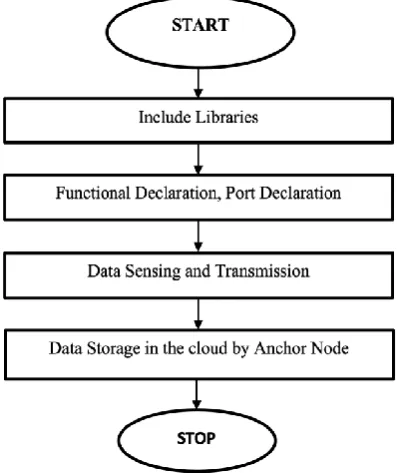
II. 3D VISUALIZATION USING AQUA-3D Aqua-3D (NAM) is a 3D network visualization tool used for visualizing underwater simulations. Aqua-3D [4] has been developed as an alternative to Aqua-Sim network simulator (NS-2 based) and it is used to simulate underwater acoustic networks. Aqua-3D has data manager CCP tool with built-in functions using which a waterbed environment can be created. Fig. 1 shows the flow chart of the localization process using Aqua-3D. In the deployed network [6], clusters are formed each with an anchor node as cluster head that knows its position coordinates apriori and has the highest battery power. The other non-localized nodes in the cluster are localized using recursive localization with anchor node position as reference. Clusters are given ID numbers based on their position in the 3D environment. For example cluster having x,y,z polarity values as +++ is given ID 1, x,y,z polarity values as ++- is given ID 2 and so on. For simulation experiments, maximum of 8 clusters is considered. Each node position is finally determined in terms of x,y,z coordinates. Data manager stores the location values of sensor nodes recursively, and these values can be seen in the node details window.
3D Localization and Visualization of Sensor
Nodes and Data Sensing in Underwater Wireless
Sensor Networks
Networks
In case there is change in the network topology because of node movements, localization procedure is repeated beginning with cluster formation. [image:2.595.68.270.98.332.2]Fig. 1. Flowchart of the Localization Process NS-3 is used for simulator node deployment and network animator tool Aqua-3D for 3D visualization and localization coordinates. Table-I shows the simulation parameters considered for Aqua-3D simulations. Fig. 2 shows the 3D model of the deployed UWSN.
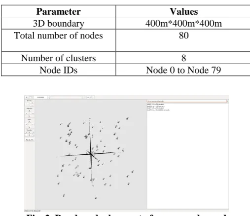
Table-I: Simulation Parameters
Parameter Values
3D boundary 400m*400m*400m Total number of nodes 80
Number of clusters 8
Node IDs Node 0 to Node 79
Fig. 2. Random deployment of sensor nodes and environment details
[image:2.595.321.530.305.695.2]After setting the environment details, using data manager CCP tool, water environment is created. Fig. 3 shows the 3D network grid having the deployed nodes. During simulation, nodes are initiated to move randomly in the water environment.
Fig. 3. Network grid with sensor nodes
The deployed nodes are then grouped into 8 clusters, each cluster having a finite number of nodes. The node with the highest battery power is considered as the anchor nodes designated with node numbers 0, 10, 20, 30, 40, 50, 60 and 70. For clarity, the various nodes are differentiated in the grid using different size, shape and colour, as indicated in Fig. 4. The node ID details such as node position, velocity, and stop time of the simulation, can be seen in the node details window in Fig. 4 (a), 4 (b) and 4 (c).
4 (a)
4 (b)
4 (c)
Fig. 4. Sensor node details
[image:2.595.40.294.431.650.2]International Journal of Innovative Technology and Exploring Engineering (IJITEE) ISSN: 2278-3075,Volume-8 Issue-12, October, 2019
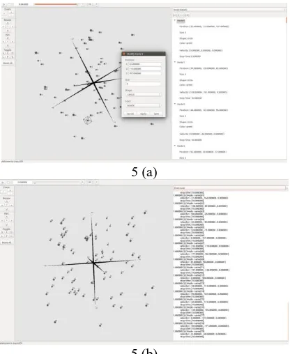
During simulation, though all the sensor nodes move randomly in the grid structure, anchor nodes are static as shown in Fig. 5. The anchor nodes exchange information with other nodes in the cluster. Also, the time information for each node deployed can be observed.
5 (a)
[image:3.595.65.273.119.373.2]5 (b)
[image:3.595.320.531.143.306.2]Fig. 5. Anchor node coordinates and timing details Subsequently, the location of the non-localized nodes gets updated recursively as in Fig. 6. For example, if node 69 is considered, initially, it was at position (-48.00,-116.00,103.00). After 30 seconds of simulation time, the position gets updated to (296.22,220.14,54.00) and so on. The non-localized node is successfully localized, and 3D coordinates are obtained.
Fig. 6. Localization details of non-localized node
III. HARDWARE EXPERIMENTATION
Experiments have been conducted by deploying the non-localized nodes underwater to a depth of 1-4 meters and anchor node placed on the surface of the water body. We have used a linux operating system with a 2GB graphics card for uninterrupted simulation. It is also installed with all the required software including VNC Viewer to to act as an anchor node.
The non-localized anchor node has the following hardware components interconnected, as shown in Fig. 7. It consists of
a. Raspberry Pi 3 b+.
b. A TFT display to observe the output offshore. c. A GPS module for obtaining the 3D coordinates. d. Temperature sensor named DHT-11.
e. Battery (Power Bank).
[image:3.595.67.275.494.609.2]This whole setup is placed in IP67 rated electrically harnessed waterproof enclosure.
Fig. 7. Hardware components of the non-localized sensor node
The anchor node fetches its position coordinates from GPS and interacts with the non-localized nodes. The 3D coordinates are iteratively determined for the 6 sensor nodes deployed underwater. As a case study for data transmission in the network, temperature sensors have been placed in the non-localized node. Over the network of non-localized nodes, 3D localization performed helps in routing the data. The water temperature is measured and transmitted to the anchor node. The temperature values is stored in the cloud and updated once in every 1 hour that can be retrieved for analysis.
The block diagram shown in Fig. 8 gives a pictorial description of the complete experimental setup. Fig. 9 shows the deployed UWSN test bed in the swimming pool of our institution.
[image:3.595.324.531.541.667.2]Networks
9 (a)
9 (b)
9 (c)
Fig. 9. Hardware test bed
[image:4.595.58.280.48.472.2]The Flow chart shown in Fig. 10 describes the experimental procedure and working of the sensor network.
Fig. 10. Python program workflow in Raspbian OS
[image:4.595.322.532.99.200.2]Python programming used for temperature date measurement and storage in the ‘smartcore’ cloud. Header format used is as shown in Fig. 11.
[image:4.595.299.556.280.357.2]Fig. 11. Data Structure for SmartCore Cloud Table-II shows the parameters considered for 3D visualization and localization using Aqua-3D simulator.
Table-II: Hardware Implementation Parameters
Parameter Values
Pool Boundary 20m*8m*3.6m Total number of nodes 6
Number of clusters 1
Node IDs Node 0 to Node 5
The experimentation is conducted for the above mentioned parameters and response of the GPS is recorded.
[image:4.595.323.532.483.602.2]Since we know the actual length, breadth and depth of the placed sensor nodes, the same information is recorded and simulations is run with Aqua-3D for exact coordinate vales. Fig. 12 shows the display of 3D coordinate node information, namely latitude, longitude and depth and also the temperature measured at the anchor node. Also, the same information is updated in the smartcore cloud. Also, the GPS values are observed using VNC viewer.
Fig. 12. 3D coordinates and temperature obtained for the non-localized sensor node
[image:4.595.68.267.523.760.2]International Journal of Innovative Technology and Exploring Engineering (IJITEE) ISSN: 2278-3075,Volume-8 Issue-12, October, 2019
Table-III: Latitude, Longitude and Depth Values of Aqua-3D and GPS
Node IDs Latitude Longitude Depth
Aqua-3D GPS Difference Aqua-3D GPS Difference Aqua-3D GPS Difference
0 87.8 87.9 0.1 179.6 179.5 0.1 0.5 0.7 0.2
1 70 70.1 0.1 118.3 118.3 0 0.9 0.8 0.1
2 12.9 12.9 0 76.2 76.1 0.1 1.3 0.9 0.4
3 -36.6 -36.6 0 -67.3 -67.4 0.1 1.8 1.1 0.7
4 -55.5 -55.6 0.1 -95.4 -95.3 0.1 2.7 1.7 1
5 -80.6 -80.6 0 -163.9 -163.9 0 3.2 1.9 1.3
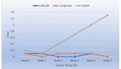
Difference in values for latitude and longitude is minimal. However, as the depth increases, the difference (error) in depth values is increasing, as shown in Fig. 13.
Fig. 13. Comparative analysis of Aqua-3D and GPS measurements
The error gets increased as the depth increases probably because radio frequency GPS signals get attenuated underwater.
IV. CONCLUSION
Aqua-3D simulator is a useful tool that provides 3D coordinates of sensor nodes underwater. Experiments have been successfully conducted to obtain 3D coordinates of the underwater sensor nodes. The temperature data obtained is transmitted successfully to anchor nodes for analyzing and storage in smartcore cloud platform. Aqua-3D values are compared with the GPS values for latitude, longitude values but difference in the depth values increases with increase in the depth probably because of attenuation of GPS values.
ACKNOWLEDGMENT
This work is carried out with the support of Department of E & C Engineering, Malnad College of Engineering, Hassan and Pincore Technologies India Pvt. Ltd., Bengaluru.
REFERENCES
1. Felemban, E. Shaikh, F. K. Qureshi, U. M. Sheikh, A. A. Qaisar, S. B.,
“Underwater sensor network applications: A comprehensive survey”, Int. J. Distrib. Sens. Netw. 2015, 2015, pp.1–14.
2. Kumar R., Singh N., “A survey on data aggregation and clustering
schemes in underwater sensor networks”, Int. J. Grid Distrib. Comput. 2014, 7, pp. 29–52.
3. N. Yashwanth and B. R. Sujatha, “Wireless Sensor Node Localization
in Underwater Environment”, IEEE International Conference on Electrical, Electronics, Communication, Computer and Optimization Techniques (ICEECCOT) 2016, IEEE ISBN 978-1-5090-4697-3, pp. 339-344.
4. Matthew Tran, Michael Zuba, Son Le, Yibo Zhu, Zheng Peng and
Jun-Hong Cui, “Aqua-3D: An Underwater Network Animator”, IEEE Oceans Conference, 2012.
5. Z. Peng, S. Le, M. Zuba, H. Mo, Y. Zhu, L. Pu, J. Liu and J. H Cui,
“Aqua-TUNE: A Testbed for Underwater Networks,” Proc. of IEEE/OES OCEANS’11 - Spain, June 2011.
6. N. Yashwanth and B. R. Sujatha, “Node Localization Performance for
UWSN Topologies,” Journal of Communications, vol. 14, no. 9, August 2019, pp. 839-844.
7. J. Yang, C. Zhang, X. Li, Y. Huang, S. Fu, M.F. Acevedo, "Integration
of wireless sensor networks in environmental monitoring cyberinfrastructure", Wireless Networks, Springer/ACM, Volume 16, Issue 4, May 2010, pp. 1091-1108,
8. G. Werner Allen, P. Swieskowski, M. Welsh. “MoteLab: A wireless
sensor network testbed”, Fourth International Symposium on Information Processing in Sensor Networks, April 2005, pp. 483-488.
9. Sheikh Ferdoush, Xinrong Li “Wireless Sensor Network System
Design using Raspberry Pi and Arduino for Environmental Monitoring Applications”, Elsevier The 9th International Conference on Future Networks and Communications (FNC-2014).
10. X. Wei, J. Liu, G. Zhang. "Applications of web technology in wireless
sensor network", The 3rd IEEE InternationalConference on Computer Science and Information Technology (ICCSIT), 2010, pp. 227-230. 11. Singh, R., Mishra, S., "Temperature monitoring in wireless sensor
network using Zigbee transceiver module," Power, Control and Embedded Systems (ICPCES), 2010.
12. Zhang Ruihua, Yuan Dongfeng “Embedded wireless sensor network
node design”, Computer Engineering, 2007, 283-285
13. Nikhade, Sudhir G. Agashe, A. A., “Wireless sensor network
communication terminal based on embedded Linux and Xbee,” Circuit, Power and Computing Technologies (ICCPCT), 2014.
14. Erol Kantarci, M. Mouftah and H. T. Oktug, "A survey of architectures
and localization techniques for underwater acoustic sensor networks". IEEE Commun. Surv. Tutor, 2011, pp. 487–502.
15. M. Garcia, S. Sendra, M. Atenas and J. Lloret, “Underwater wireless
ad-hoc networks: A survey," Mobile ad hoc networks: Current status and future trends, 2011, pp. 379-411.
16. Z. Zhou, Z. Peng, J. H. Cui, Z. Shi and A. Bagtzoglou, “Scalable localization with mobility prediction for underwater sensor networks," IEEE Transactions on Mobile Computing, vol. 10, no. 3, 2011, pp. 335-348.
17. Z. Zhu, W. Guan, L. Liu, S. Li, S. Kong and Y. Yan, “A multi-hop localization algorithm in underwater wireless sensor networks," in Wireless Communications and Signal Processing (WCSP), Sixth International Conference on. IEEE, 2014, pp. 1-6.
18. A. Sheinker, B. Ginzburg, N. Salomonski, L. Frumkis and B. Z.
Kaplan, "Localization in 3-d using beacons of low-frequency magnetic field," IEEE Transactions on Instrumentation and Measurement, vol. 62, no. 12, 2013, pp. 3194-3201
19. M. Zuba, Z. Shi, Z. Peng, J. Cui and S. Zhou, “Vulnerabilities of Underwater Acoustic Networks to Denial-of-Service Jamming Attacks.” in Wiley Security and Communication Networks, February 2012, pp. 1– 10.
20. “Aqua-3d official wiki,” November 2010. [Online]. Available:
http://obinet.engr.uconn.edu/wiki/index.php/Aqua-3D
21. SmartCore webpage:
[image:5.595.64.274.249.369.2]Networks
AUTHORS PROFILEMr. N. Yashwanth obtained his B.E. degree from Kalpataru Institute of Technology, Tiptur in 2010 and M.Tech from School of Engineering and Technology, Jain University in 2012. He is currently working as an Assistant Professor in the Department of Electronics and Communication Engineering at Rajeev Institute of Technology, Hassan. He is pursuing PhD under the supervision of Dr. B R Sujatha in the area of underwater wireless sensor networks in the Department of Electronics and Communication Engineering at Malnad College of Engineering, Hassan. His research interests are Signal Processing, Communication Systems and Wireless Sensor Networks.