FILMPAR: A parallel algorithm designed for the efficient and accurate computation of thin film flow on functional surfaces containing micro-structure

promoting access to White Rose research papers

White Rose Research Online

Universities of Leeds, Sheffield and York

http://eprints.whiterose.ac.uk/

This is an author produced version of a paper published in Computer Physics Communications Package.

White Rose Research Online URL for this paper: http://eprints.whiterose.ac.uk/10469

Published paper

Lee, Y.C., Thompson, H.M. and Gaskell, P.H. (2009) FILMPAR: A parallel algorithm designed for the efficient and accurate computation of thin film flow on functional surfaces containing micro-structure. Computer Physics

FILMPAR: A parallel algorithm designed for

the efficient and accurate computation of thin

film flow on functional surfaces containing

micro-structure

Y C Lee

, H M Thompson

, P H Gaskell

a_{School of Mechanical Engineering, The University of Leeds, Leeds, United}

Kingdom. LS2 9JT

Abstract

A highly efficient and portable parallel multigrid algorithm for solving a discre-tised form of the coupled lubrication equations for three-dimensional, gravity-driven, continuous thin film free-surface flow over substrates containing micro-scale topog-raphy is presented. Although applicable to problems involving heterogeneous and distributed features, for illustrative purposes the algorithm is benchmarked for the case of flow over a single trench topography; this enables direct comparisons with complementary experimental data and existing serial multigrid solutions. Parallel performance is accessed and shown to lead to super-linear behaviour provided the finest multigrid mesh level employed is sufficiently so.

Key words: Multigrid, parallel computing, thin film flow, lubrication equations

PROGRAM SUMMARY

Manuscript Title: FILMPAR: A parallel algorithm designed for the efficient and accurate computation of thin film flow on functional surfaces containing micro-structure

Authors: P.H. Gaskell, Y.C. Lee, H.M. Thompson

Program Title:FILMPAR

Journal Reference: Catalogue identifier: Licensing provisions: none

Programming language: C++

Computer: Desktop, server

Operating system:Unix/Linux, Mac OS X

RAM:512 Mbytes

Number of processors used: 128

Supplementary material:

Keywords:Multigrid, parallel computing, thin film flow, lubrication equations, adap-tive time-stepping

PACS:

Classification:12

External routines/libraries:GNU C/C++, OpenMPI

Subprograms used:

Catalogue identifier of previous version:*

Journal reference of previous version:*

Does the new version supersede the previous version?:*

Nature of problem:

Thin film flows over functional substrates containing well-defined single and com-plex topographical features are of enormous significance, having a wide variety of engineering, industrial and physical applications. However, despite recent modelling advances, the accurate numerical solution of the equations governing such problems is still at a relatively early stage. Indeed, recent studies employing a simplifying long-wave approximation have shown that highly efficient numerical methods are necessary to solve the resulting lubrication equations in order to achieve the level of grid resolution required to accurately capture the effects of micro- and nano-scale topographical features.

Solution method:

A portable parallel multigrid algorithm has been developed for the above purpose, for the particular case of flow over submerged topographical features. Within the multigrid framework adopted, a W-cycle is used to accelerate convergence in the re-spect of the time dependent nature of the problem, with relaxation sweeps performed using a fixed number of pre- and post- Red-Black Gauss-Seidel Newton iterations. In addition, the algorithm incorporates automatic adaptive time-stepping to avoid the computational expense associated with repeated time-step failure.

Reasons for the new version:*

Summary of revisions:*

Restrictions:

Unusual features:

Additional comments:

Running time:

million nodes.

References:

1 Introduction

The accurate prediction of the free-surface disturbance arising from the flow of a continuous thin liquid film over functional substrates containing regions of micro- or nano-scale topography presents a considerable challenge given that the same can persist over length scales several orders of magnitude greater than the topography itself [1–3]. The problem becomes further exacerbated when the features concerned are: (i) small, thus requiring considerable mesh resolution to achieve the necessary level of solution accuracy and mesh inde-pendence; (ii) heterogeneous, covering a wide extent of the substrate’s surface.

The above has motivated the development of an efficient, fully-implicit multi-grid strategy for investigating such flows, by solving the lubrication equation(s) that result from using the long-wave approximation to simply the governing Navier-Stokes equations under the assumption that the ratio of the undis-turbed asymptotic film thickness to that of the characteristic in-plane length scale is small, coupled with the neglect of inertia. The approach has been shown to be very robust and to return an order of magnitude, or more, im-provement in the rate of convergence compared to ADI schemes [4], the bene-fits of which can be further enhanced by adopting error-controlled automatic adaptive time-stepping [5] and/or adaptive mesh refinement [6].

Described below is a new portable parallel multigrid lubrication flow solver that has been developed to solve continuous thin film flows over submerged topography. Benchmark results are presented, compared against complemen-tary experimental data and results obtained from serial multigrid predictions of the free-surface disturbance, which demonstrate the accuracy of the par-allel implementation. The parpar-allel performance of the solver, executed on a distributed memory IBM BlueGene/P computing platform, is assessed and shown to lead to super-linear behaviour provided the finest mesh level em-ployed in the multigrid approach is sufficiently so.

2 Theoretical background

2.1 Mathematical formulation and problem specification

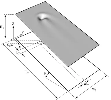
Cartesian coordinate system (X, Y, Z) at time, T, over a substrate of width,

Wp, length,Lp, isH(X, Y, T); the constant volumetric flow per unit width

be-ing Q0. The substrate is inclined at an angleθ to the horizontal and contains,

for illustration purposes, a single rectangular trench topography, S(X, Y), of depth,S0. The liquid is assumed Newtonian and incompressible with constant

viscosity, µ, density, ρ, and surface tension, σ.

A generic set of governing equations, based on the long-wave lubrication ap-proximation, for thin-film flow is derived. By proceeding as in [6], the governing Navier-Stokes equations simply considerably by neglecting inertia and assum-ing that ǫ = H0/L0 is small, where L0 is the characteristic in-plane length

scale, proportional to the capillary length, Lc, given by:

L0 =β

σH0

3ρgsinθ !1/3

and β =L0/Lc , (1)

with H0 = (3µQ0/ρgsinθ)1/3, the undisturbed Nusselt film thickness; where

g is the acceleration due to gravity.

Neglecting terms of O(ǫ2_{) and smaller and imposing no-slip conditions and}

zero tangential shear stress at the substrate and free-surface, respectively, and using the following scalings [7], (x, y) = (X, Y)/L0, h = H/H0, t = U0T /L0,

U0 = 3Q0/2H0, s = S/H0 and p = 2P/ρgL0sinθ, results in the following

equation forh:

∂h ∂t = ∂ ∂x ( h3 3 ∂ ∂x "

−_β6₃ ∂

2_ψ

∂x2 +

∂2_ψ

∂y2

!

+ 2

β6

1/3_Nψ

#

− 2₃h3 ) + ∂ ∂y ( h3 3 ∂ ∂y "

−_β63

∂2_ψ

∂x2 +

∂2_ψ

∂y2

!

+ 2

β6

1/3_Nψ

#)

, (2)

where ψ = h +s. Alternatively, the above can be written as a coupled set of equations for h and p, the pressure throughout the film, which from the standpoint of computational efficiency has been shown to be preferable [8]:

∂h ∂t = ∂ ∂x " h3 3 ∂p ∂x −2

!# + ∂ ∂y " h3 3 ∂p ∂y !# , (3)

p=₋ 6

β3∇

2_{(ψ) +} 2

β6

1/3_{N(ψ) , (4)}

with the pressure datum is set to zero; N = Ca1/3_{cotθ measures the}

(9µ2_Q2

0/8ρgσ3sinθ)1/3 is the Capillary number.

2.2 Topography specification

Following [9], the topography depth, s, is defined via an arctangent function which enables the side steepness to be controlled easily, thus providing the flex-ibility needed to create simple primitive shapes [6]. For example, the rectan-gular topography shown in Figure 1, of lengthlt =LT/L0, widthwt =WT/L0

and height, s0 =S0/H0, centred at point (xt, yt), is specified by defining:

s(x, y) =s0

b0

"

tan−1 −ax−lt/2

γlt

!

+ tan−1 ax−lt/2

γlt

!#

×

"

tan−₁ −ay −wt/2

γwt

!

+ tan−₁ ay−wt/2

γwt

!#

, (5)

whereγis an adjustable steepness parameter,b0 = 4 tan

−₁

(1/2γ) tan−₁

(A/2γ),

A =wt/lt is the aspect ratio and ax = xt−x and ay = yt−y are the local

topography co-ordinates in thex- and y-directions, respectively.

Equation (5) can be used to specify other simple primitive topography shapes such as elliptic or lozenge shapes by modifying ax and ay appropriately. It is

then relatively straightforward to add and subtract these primitives to create complex topographical patterns to represent realistic engineering functional substrates [10].

2.3 Boundary conditions

The problem is closed by specifying appropriate boundary conditions and assuming developed flow conditions to exist far upstream, namely:

h(x= 0, y) = 1, (6)

while imposing zero normal flux conditions at the other streamwise and span-wise boundaries yield:

∂h ∂n =

∂p

2.4 Spatial discretisation

The lubrication equations (3) and (4) are discretised using a central finite-difference scheme with uniform grid spacing, ∆, in both thex- andy-directions; leading to the following second order accurate spatial analogues for hand p:

∂hi,j ∂t = 1 ∆2 h3 3 _i+1

2,j

(pi+1,j−pi,j)−

h3

3

_i−1

2,j

(pi,j −pi−_1,j) +

h3

3

_i,j+1

2

(pi,j+1−pi,j)−

h3

3

_i,j−1

2

(pi,j −pi,j−₁)

− 2 ∆ h3 3

i+1 2,j − h 3 3

i−1 2,j

, (8)

pi,j=−

6

β3_∆2

(hi+1,j +si+1,j) + (hi−_1,j+s_i−_1,j) + (h_i,j+1+s_i,j+1) +

(hi,j−₁+s_i,j−₁)−4(h_i,j+s_i,j)

+2

3

√

6N

β (hi,j+si,j) , (9)

at each node, (i, j), in the computational domain. The pre-factor terms, h3

3 |i±1

2,j

and h₃3|i,j±1

2, are obtained from linear interpolation between neighbouring

points.

2.5 Temporal discretisation

Time integration is performed using the second-order accurate Crank-Nicholson method to approximate the time-derivative of equation (8) and which, rewrit-ing the right-hand-side as a function, _F(hi,j, pi,j, hi±_1,j, p_i±_1,j, h_i,j±₁, p_i,j±₁),

leads to an equation of the form:

hn_i,j+1₋∆t

n+1

2 F(h

n+1

i,j , pni,j+1, hni±+1_1,j, p n+1

i±_1,j, h n+1

i,j±₁, p n+1

i,j±₁)

=hn_i,j +∆t

n+1

2 F(h

n

i,j, pni,j, hni±_1,j, pn_i±_1,j, hn_i,j±₁, pn_i,j±₁), (10)

where ∆tn+1 _=tn+1_−tn_{; the right hand side of the above equation is expressed}

in terms of known variables at the end of the nth time step, t=tn_.

method employed provides an efficient alternative to existing schemes such as [11] by using time-stepping based on local error estimates, one that is im-plicit and second order accurate, obtained from the difference between the current solution and predicted one and which act as an indicator of whether to increase or decrease the time step in a controlled manner whilst concur-rently minimising the computational expense associated with repeated time step failure.

2.6 Multigrid strategy

In line with the multigrid algorithm employed in [6], a sequence of progressively finer grids (Gk:k = 0,1, ..., K) is defined with uniform grid spacing, ∆k. Each

grid level, _Gk, has nk = 2k+c+1+ 1 nodes per unit length in each co-ordinate

direction, where c is a constant defining the resolution of the coarsest grid level such that mesh size, ∆k = 2

−_(k+c+1)

.

The associated time-dependent, nonlinear, coupled set of governing lubrication equations (9) and (10) are solved using a full approximation storage (FAS) multigrid scheme [12]. By combining and re-writing the above set of discretised equations as follows:

Nkunk+1 =fk(unk) (11)

where uk = (hk, pk)T with Nk = (Nkh,N p

k)T and fk = (fkh, f p

k)T corresponds

to the left- and right-hand sides of the both the film thickness and pres-sure equations on Gk, respectively, the multigrid method can be summarised

schematically, as in Algorithm 1.

Note that the cycle-index, κ, which represents the number of iterations of the multigrid process at each intermediate grid level, determines the type of coarse grid correction cycle. Here, the W-cycle (κ= 2) is employed to optimise the convergence properties provided by the scheme for the time-dependent lubrication solution.

The inter-grid transfer operators used in the multigrid algorithm consist of restriction operator Rk−₁

k (from Gk to Gk−₁) and prolongation operator, I_kk−₁

(grid_Gk−₁toG_k), whose orders depend on the order of derivatives being solved.

For the second order lubrication equations under consideration, the standard half-weighting restriction and bi-linear interpolation are appropriate.

In order to avoid convergence problems that may arise from using an arbitrary initial guess, the Full Multigrid (FMG) technique [12] is used together with the FAS algorithm, see Algorithm 2. Note that Πk

for transferring information from Gk−₁ toG_k and its order may not necessary

be equal to that of the prolongation operatorIk k−₁.

2.7 Relaxation

Relaxation is performed using a fix number, (ν1, ν2), of pre- and post-

Red-Black Gauss-Seidel Newton iterations with the linearised Newton iterative step written in the form:

∂_Nh k

∂hn_k+1∆hk+ ∂_Nh

k

∂pn_k+1∆pk=f

h

k − Nkh(hnk, pnk) , (12)

∂_Nkp

∂hn_k+1∆hk+ ∂_Nkp

∂pn_k+1∆pk=f

p k − N

p

k (hnk, pnk) , (13)

for the increments ∆h and ∆p at point (i, j) on level k. The expressions are then solved simultaneously to obtain a new approximate solution on _Gk:

˜

hn_k+1 =hn_k+1+ ∆hk , (14)

˜

pn_k+1 =pn_k+1+ ∆pk . (15)

2.8 Parallel implementation

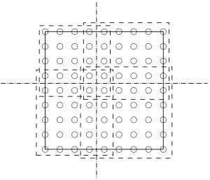
Parallel implementation of the above automatic adaptive time-stepping multi-grid solver is achieved through the use of a message passing interface (MPI) framework, which facilitates portability across different (distributed and shared memory) high performance computing platforms. Parallelism is achieved via a geometric partitioning at each of the grid levels, using a strategy that automat-ically constructs virtual topologies arranged so as to minimise communication cost. This is illustrated in Figure 2, where the partitions, depending on the number of processors and shape of the domain, are split into, or as close as is possible, equally divisible rectangular blocks. Note that when the number of columns or rows is not an exact multiple of the number of processors used, the left over points are allocated to the last processor associated with the respective rows and columns.

after the inter-grid transfer operations. Additionally, a global communication exchange is performed at the end of each multigrid cycle to ascertain whether a converged solution has been achieved.

The above approach allows standard sequential algorithms, such as the FMG-FAS multigrid scheme to be parallelised without any fundamental alteration, as the assembly of the underlying discrete system of equations is undertaken by the initial domain decomposition process; maintaining this strategy for the parallel solver minimises the need for data movement within a distributed memory parallel code. Nonetheless, obtaining good parallel efficiencies for such a scheme is challenging due to the fact that several computations must be undertaken on relatively coarse meshes which may result in an undesirably large communication overhead.

3 Benchmark numerical results

The benchmark test problem considered is that of the gravity-driven flow of a thin film of water (viscosity, µ = 0.001 Pa s, density, ρ = 1000 kg m−₃

and surface tension, σ = 0.07 N m−₁

), having an asymptotic film thickness

H0 = 100µm, over a rigid substrate (of sizelp =wp = 100 and tilted at 30o to

the horizontal) containing a single localised, square trench topography (γ = 0.05, so = −0.25, and lt = wt = 1.54), centred at (xt, yt) = (30.77,50). The

above fluid properties and associated flow parameters are consistent with the experiments carried out by [1] enabling direct comparison with the same and with complementary numerical predictions obtained using a serial multigrid algorithm [6] employing automatic mesh adaption. The values for Lc = L0

and N are 0.78 mm and 0.12, respectively; the latter indicting the normal component of gravity has little effect on the resultant free-surface shape [2].

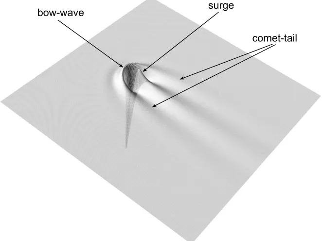
The steady-state free-surface disturbance illustrated in Figure 3 was obtained with a fine mesh containing 1025_×1025 nodes, guaranteeing an accurate grid independent solution. It shows the gross characteristic “horse-shoe” bow-wave and a “comet-tail” pattern that results. Streamwise free-surface profiles at different spanwise cross-sectional locations are depicted in Figure 4, comparing those obtained with FILMPAR against their experiment counterparts and ones obtained using a serial multigrid solver. As can be seen, the FILMPAR profiles shows very good qualitative agreement with experimental data, to within the 2% r.m.s experimental error reported in [1], and are indistinguishable from the corresponding serial multigrid solutions [6].

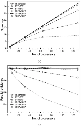
and 2 GB of local memory. Figure 5 shows the speedup and parallel efficiency of the parallel multigrid solver when executed on between 4 and 128 proces-sors, together with the theoretically expected values. The results are presented relative to the smallest number of processors used, which in this case is 4, employing 4 multigrid levels with W(2,2)-cycles. Figure 5(a) indicates that a relatively good level of speedup is achieved, as one would expect, giving better returns when finer meshes (1025×1025 and above) are employed, as opposed to coarser grids due to the considerable inter-processor communication cost incurred during coarse grid computations that lead to large computational overheads. This is more clearly shown in Figure 5(b) where parallel efficiency is seen to approach the theoretical limit when very fine grids are employed as a result of large relative computation to communication ratios especially when a larger number of processors are used. Indeed, super-linear parallel perfor-mance is observed with 16 processor for a fine mesh having 2049_×2049 points, and with 16, 32 and 64 processors when the fine mesh contains 4097×4097 points. The reason for this can be attributed to the likely fact of the efficiency of communication and cache effects, which come into play when the size of the sub-domains become small and the variables accessed fit into the cache dramatically reducing memory access times and hence computational times.

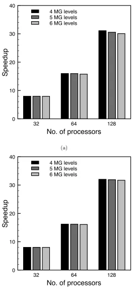
The precise choice made for size of the coarsest grid level has a bearing on the overall parallel performance. A comparison of the efficiency of FILMPAR for fine grid levels of 2049_×2049 and 4097_×4097, using different number of multigrid levels is shown in Figure 6. It reveals that the cost of performing a greater number of multigrid levels diminishes as a finer mesh is used, as indi-cated by the improved consistency in speedup efficiencies depicted in Figures 6(a) and 6(b). Speedup becomes more pronounced as the number of multgrid levels increases, particularly when a large number of processors is employed. This is more evident for the case when the finest mesh contains 2049_×2049 points, which is to be expected since the coarse grid levels utilised are coarser and thus the amount of computation per processor is smaller.

4 Conclusions

A highly accurate and efficient portable parallel multigrid lubrication solver is presented for the solution of three-dimensional gravity-driven continuous thin film free-surface flow over substrates containing topography. It enables results to be obtained on extremely fine meshes, ones that cannot be attempted using a serial solver; the solver having a parallel efficiency that is both scalable and cost effective. Benchmark results, compared against known experimental data and with existing serial multigrid solutions reveal that the parallel solver generates accurate steady-state free-surface disturbances for flow over a small trench.

The performance characteristics of the parallel solver indicate that its imple-mentation is highly efficient specifically when, as is the case of flow over small topographical features, a fine mesh is required to produce accurate mesh in-dependent solutions; small losses in efficiency that can be attributed to the overhead associated with inter-processor communication. The latter becomes apparent in the case of coarser grid levels where the amount of computation per processor is relatively small. Accordingly, given that multigrid schemes are designed do most of their work on coarser grid levels, it is important to select a fine grid level that does not compromise parallel performance.

5 Overview of the software structure

FILMPAR is written entirely using C++, making full use of its object-oriented framework to simplify the creation of arrays and variable structures as well as to allow for code flexibility and future extensibility. The program has a modular form, with routines and functions defined in separate files, as per the following structure:

./input – stores user provided input data files

./src – location of the source files

./scr/core – location of the core source files

./src/include – location of the header files

./src/lib – location of general library routines

./src/template – location of template files

6 Description of the individual software components

Core source files located at./src/core:

• ats_predict.cpp– Computes and controls the adaptive time-stepping

rou-tine.

• ats_set.cpp – Initialises and defines variables h and p for the new time

step.

• engine_clean.cpp – Uninitialise the grid arrays used and free up memory.

• engine_init.cpp–Initialise the grid arrays, topography and initial profiles of the thin film flow problem.

• engine_mpi_mg.cpp – Performs a full multigrid (FMG) iteration and

de-termine if additional multigrid iterations are required.

• engine_mpi_solver.cpp – Performs the adaptive or non-adaptive

time-stepping routine on the multigrid algorithm.

• engine_mpi_write.cpp – Determine types of output data.

• engine_parameters.cpp – Calls read, process and write input parameter

data.

• evalpressure.cpp – Calculates initialp fromh and s values.

• func_mpi_lop.cpp – Calculates _Nkunk+1.

• func_mpi_rhs.cpp – Calculates fn

k.

• grids_init.cpp – Initialises arrays and grid structure for parallel

imple-mentation.

• grids_mpi_reset.cpp – Resets temporary arrays.

• mg_mpi_cycle.cpp – Performs the parallel multigrid cycle with calls to

appropriate relaxation and interpolation operators.

• mg_mpi_lop.cpp– Sets up domain boundaries and callsfunc_mpi_lop.cpp.

• mg_mpi_relax.cpp – Set up domain boundaries and callsnewtitr.cpp.

• mg_mpi_solve_coarsest.cpp – Performs multiple relaxation iterations for

coarsest grid solution.

• mg_mpi_solve_rhs.cpp – Setup domain and calls func_mpi_rhs.cpp.

• mpi_init.cpp – Initialises and sets up the parallel environment variables.

• mpi_uninit.cpp – Uninitialise the parallel environment variables.

• newtitr.cpp – Performs relaxation using Newton iteration on the coupled

system of equationsh and p.

• nonats_set.cpp– Sets up appropriate variables and arrays for non-adaptive

time-stepping.

• parameters_mpi_write.cpp – Creates and sets up appropriate directories

for parameter output files.

• parameters_process.cpp– Calculates and processes the input parameters

used.

• parameters_read_tag.cpp – Defines the tags that are read from the input

parameter file.

• parameters_write_tag.cpp – Writes out the processed information and parameters used.

• parameters_write.cpp – Creates and writes the parameters used into a

file.

• pre.cpp – Performs the exchange of halo data from initial h,p and s.

• profiles_film.cpp – Specifies and sets up the initial profile for the thin

film flow problem.

• profiles_init.cpp – Initialises the definition of the thin film profile.

• topography_init.cpp – Sets up the topography input file for reading.

• topography_read.cpp – Reads in the parameters from the input

topogra-phy file.

• topography_set.cpp – Creates and processes the topography information

read from the input file.

• write_data_array.cpp – Writes parallel output data to file.

• write_mpi_create_mesh.cpp – Determines the types of output files.

• write_mpi_data.cpp– Creates and prepares the appropriate filenames and

data for parallel output.

• xmg_main.cpp – The main file that performs the time-adaptive parallel

multigrid solver.

Library source files located at./src/lib:

• anorm2_mpi.cpp – A function that returns the _L2_{-norm value.}

• copy_mpi.cpp – Duplicates a grid array variable.

• interp_mpi.cpp– Performs the bilinear interpolation of grid variables from a coarse to fine grid.

• matadd_mpi.cpp – Calculates the addition of two grid array variables.

• matsub_mpi.cpp – Calculates the subtraction of two grid array variables.

• rstrct_mpi.cpp– Performs the half-weighting restriction of grid variables

from a fine to coarse grid.

• rstrctinject_mpi.cpp – Performs the injection of grid variables from a

fine to coarse grid.

Header files located at ./src/include:

• incl_core_header.h – Provides the namespace for all the core source files.

• incl_grids.h – Defines the structure of the array variables and parallel

parameters.

• incl_lib_header.h – Provides the namespace for all the library source

files.

• incl_parameters.h – Defines all the parameters used in the program.

• incl_template.h – Defines the one- and two-dimensional array template

structures.

• tmpl_array_1d.h – Defines the template and class for one-dimensional ar-rays.

• tmpl_array_2d.h– Defines the template and class for two-dimensional

ar-rays.

• tmpl_io_check.h – Defines the template class for input and output file

checking.

• tmpl_level_define.h – Defines the template class for various multigrid

array structures.

Input files located at ./input:

• xmg-parameter.input– Defines the input flow, multigrid and domain

vari-ables.

• xmg-topography.input – Defines the shape and size of the topography.

7 Installation instructions

The code can be compiled on any system with a GNU C++ compiler and OpenMPI libraries installed, by invoking the following command:

$ make

All the files will be compiled and linked to produce an output binary executable file named filmpar.

Invoking the command:

$ make clean

will remove all compiled object files while

$ make clean-all

removes both the compiled object files and the executable binary.

8 Test run description

The binary executable file can be executed on a parallel system with multiple processors by invoking, as an example:

in which, 8 processors are allocated and utilised for the execution of the

pro-gram based on the user defined inputs provided in files./input/xmg-topography.input

and ./input/xmg-paramters.input, respectively.

All data outputs are stored in the./outputdirectory with each set of results generated by the program automatically stored in their respective subdirecto-ries; the first set of results is stored under the sub-directory./output/result

while subsequent results generated from the execution of the program are stored in sub-directories labelled result0, result1, . . . , increments.

The output files created in the result sub-directories consist of an output file

./output/result/xmg-parameters.output, which prints out the parameter

variables used by the program, and the associated output data files computed on each processor labelled in their respective sub-directories beginning with

./output/result/rank0,./output/result/rank1, . . . ,./output/result/rank7,

if 8 processors are used.

9 Acknowledgements

The authors wish to record their gratitude to the Engineering and Physi-cal Sciences Research Council (EPSRC) for supporting this work via grant reference EP/F010745/1. The authors also wish to thank Dr. XJ Gu and Pro-fessor DR Emerson (Daresbury Laboratory, Warrington, UK) for informative discussions surrounding parallel computing issues and for access to and use of the Bluegene/P high performance computing platform for benchmarking purposes.

References

[1] M.M.J. Decre, C-J. Baret, J. Fluid Mech. 487 (2003) 147.

[2] P.H. Gaskell, P.K. Jimack, M. Sellier, H.M. Thompson, M.C.T. Wilson, J. Fluid Mech. 509 (2004) 253.

[3] M. Sellier, Y.C. Lee, H.M. Thompson, P.H. Gaskell, Comput. & Fluids 38 (2009) 171.

[4] L.W. Schwartz, R.R. Eley, J. Colloid Interface Sci. 202 (1998) 173.

[5] P.H. Gaskell, P.K. Jimack, M. Sellier, H.M. Thompson, Int. J. Num. Meth. Fluids 45 (2004) 1161.

[6] Y.C. Lee, H.M. Thompson, P.H. Gaskell, Comput. & Fluids 36 (2007) 838. [7] A. Oron, S.H. Davis, S.G. Bankoff, Reviews of Modern Physics 69 (1997) 931. [8] N. Daniels, P. Ehret, P.H. Gaskell, H.M. Thompson, M.M.J. Decre, in:

[9] L.M. Peurrung, G.G. Graves, IEEE Trans. Semi. Man. 6 (1993) 72.

[10] Y.C. Lee, H.M. Thompson, P.H. Gaskell, Int. J. Num. Meth. Fluids 56 (2008) 1375.

[11] J.A. Diez, L. Kondic, J. Comput. Phys. 183 (2002) 274.

˜

un_k+1 = MGFASCYC(un_k+1, f_kn+1) 1: pre-relaxation

perform ν1 relaxation sweeps on unk+1

2: coarse grid correction

compute residual dn_k+1 =f_kn+1_{− Nk}n+1un_k+1 on _Gk

restrict residual dn_k+1−₁ =Rk −₁

k dnk+1 ontoGk−₁

restrict fine grid solution un_k−+1₁ =R k−₁

k unk+1 ontoGk−₁

compute right-hand side f_kn−+1₁ =dn_k−+1₁ +N_kn−+1₁un_k+1 on Gk−₁

If k = 0, solve for ˜un₀+1 on_G0

elseperform κ iterations on ˜un_k−+1₁ = MGFASCYC(u_kn−+1₁, f_kn−+1₁)

endif

compute correction en_k+1−₁ = ˜un_k−+1₁ −un_k+1−₁ on Gk−₁

interpolate en_k+1 =Ik k−₁e

n+1

k−₁ ontoGk

update solution un_k+1 =u_kn+1+en_k+1 on Gk

3: post-relaxation

perform ν2 relaxation sweeps on unk+1

1: for k = 0,1,2, . . . , K

2: if k = 0, solve for ˜un0+1 on G0

3: else interpolateun_k+1 = Πk k−₁u˜

n+1

k−₁ onto Gk

4: compute ˜un_k+1 = MGFASCYC(un_k+1, f_kn+1)

5: endif

6: done

0 10 20 30 40 50 60 x

-0.3 -0.2 -0.1 0 0.1

h*

Experiment Serial Multigrid FILMPAR

(a)

0 10 20 30 40 50 60

x -0.3

-0.2 -0.1 0 0.1

h*

Experiment Serial Multigrid FILMPAR

(b)

0 10 20 30 40 50 60

x -0.3

-0.2 -0.1 0 0.1

h*

Experiment Serial Multigrid FILMPAR

(c)

Fig. 4. Comparison of experimentally obtained [1] and predicted FILMPAR and serial multigrid solutions [6] streamwise free-surface film thickness profile, h∗

0 20 40 60 80 100 120 No. of processors

0 5 10 15 20 25 30

Speedup

Theoretical 257x257 513x513 1025x1025 2049x2049 4097x4097

(a)

0 20 40 60 80 100 120

No. of processors

0.4 0.6 0.8 1

Parallel efficiency

Theoretical 257x257 513x513 1025x1025 2049x2049 4097x4097

(b)

32 64 128

No. of processors

0 10 20 30 40

Speedup

4 MG levels 5 MG levels 6 MG levels

(a)

32 64 128

No. of processors

0 10 20 30 40

Speedup

4 MG levels 5 MG levels 6 MG levels

(b)