Spectral-spatial Feature Extraction for Hyperspectral Image Classification

for Hyperspectral Image

Classification

Jie Liang

A thesis submitted for the degree of

Doctor of Philosophy of

The Australian National University

Jie Liang

I would thank my primary supervisor Dr. Jun Zhou. Without his help, I cannot fin-ish this thesis. I received lots of help from him, including but not limited to follow-ing: discussing my research progress every week; helping me revise my conference and journal papers; purchasing new hyperspectral cameras to support my research; training me how to respond to reviews of my papers and how to review papers from other authors; confirming the chapter details of my thesis. Residing in a relatively new area, my research topic "spectral-spatial feature extraction for hyperspectral im-age classification" is quite challenging. I got stuck with my research frequently due to lack of datasets or standard evaluation methods. Jun and I had many discussions to solve those problems and explore new possibilities in the scope of my research topic. We believe that there are excellent opportunities with this topic, and it will draw much attention in the near future.

My panel chair, Associate Professor Hongdong Li, monitored my research progress and helped me complete a lot of paperwork when I was working as an external s-tudent of ANU. My co-supervisor, Associate Professor Henry Gardner, supported my research from Ph.D. application to the thesis finalization. My advisor Dr. Xavier Sirault introduced me to the advanced High-Resolution Plant Phenomics Centre and gave me opportunities to work with talented people there.

Professor Yongsheng Gao, although not in my supervising panel, actually worked as my supervisor as well. He brought me a lot of brilliant ideas and advices, not only for my research but also for my life, while I was visiting the Image Processing & Computer Vision Lab at Griffith University. He also granted me the opportunity to take part in the ARC Linkage Project on strawberry bruise detection via hyperspectral imaging. Rudi Bartels, Gilbert Eaton, and Lee Hamilton were my colleagues in the

research work. Besides that, Professor Yuntao Qian from Zhejiang University also worked as my advisor when he visited Griffith University in 2016. He inspired me a lot of ideas and helped a lot for my journal publication.

Jieqiong Hao, my girlfriend, entered my life at the toughest time of my Ph.D. studying. She kept encouraging me to insist on my research and accompanied me through a lot of difficulties. She acted as my life advisor and offered so many useful suggestions.

Back in my home country China, my uncles Guangyi Liang and Ming Liang, and aunts Junling Liang and Hong Fu greeted me now and then, comforting and encouraging me, and helped me take care of my families. Without them, I could not focus on my studying in Australia.

I would also thank my former supervisor Zhiqiang Zheng and Xiaohong Xu from National University of Defense Technology, where I got my bachelor degree. They offered me such an incredible opportunity to study abroad. They supported me during my application of Ph.D. and gave me the warm welcome every time visiting them in China. I appreciate their trust in me and recognition to my efforts.

The Chinese Scholarship Council and the Australian National University granted me the scholarship to live and study in Australia. ANU also supported me finan-cially to attend academic conferences. These precious experiences enriched my life and expanded my vision. Griffith University also supplied me with all the research resources that I needed to finish my study.

As an emerging technology, hyperspectral imaging provides huge opportunities in both remote sensing and computer vision. The advantage of hyperspectral imaging comes from the high resolution and wide range in the electromagnetic spectral do-main which reflects the intrinsic properties of object materials. By combining spatial and spectral information, it is possible to extract more comprehensive and discrimi-native representation for objects of interest than traditional methods, thus facilitating the basic pattern recognition tasks, such as object detection, recognition, and clas-sification. With advanced imaging technologies gradually available for universities and industry, there is an increased demand to develop new methods which can ful-ly explore the information embedded in hyperspectral images. In this thesis, three spectral-spatial feature extraction methods are developed for salient object detection, hyperspectral face recognition, and remote sensing image classification.

Object detection is an important task for many applications based on hyperspec-tral imaging. While most traditional methods rely on the pixel-wise spechyperspec-tral re-sponse, many recent efforts have been put on extracting spectral-spatial features. In the first approach, we extend Itti’s visual saliency model to the spectral domain and introduce the spectral-spatial distribution based saliency model for object detection. This procedure enables the extraction of salient spectral features in the scale space, which is related to the material property and spatial layout of objects.

Traditional 2D face recognition has been studied for many years and achieved great success. Nonetheless, there is high demand to explore unrevealed informa-tion other than structures and textures in spatial domain in faces. Hyperspectral imaging meets such requirements by providing additional spectral information on objects, in completion to the traditional spatial features extracted in 2D images. In the second approach, we propose a novel 3D high-order texture pattern descriptor

for hyperspectral face recognition, which effectively exploits both spatial and spectral features in hyperspectral images. Based on the local derivative pattern, our method encodes hyperspectral faces with multi-directional derivatives and binarization func-tion in spectral-spatial space. Compared to tradifunc-tional face recognifunc-tion methods, our method can describe distinctive micro-patterns which integrate the spatial and spectral information of faces.

Mathematical morphology operations are limited to extracting spatial feature in two-dimensional data and cannot cope with hyperspectral images due to so-called ordering problem. In the third approach, we propose a novel multi-dimensional morphology descriptor, tensor morphology profile (TMP), for hyperspectral image classification. TMP is a general framework to extract multi-dimensional structures in high-dimensional data. The nth_{-order morphology profile is proposed to work}

with the nth-order tensor, which can capture the inner high order structures. By treating a hyperspectral image as a tensor, it is possible to extend the morphology to high dimensional data so that powerful morphological tools can be used to analyze hyperspectral images with fused spectral-spatial information.

Acknowledgments vii

Abstract ix

1 Introduction 1

1.1 Hyperspectral Imaging . . . 1

1.2 Motivation . . . 3

1.2.1 The advance of imaging technology . . . 5

1.2.2 Demand for new hyperspectral image processing methods . . . 5

1.2.3 Challenges . . . 7

1.3 Objective . . . 9

1.4 Contribution . . . 10

1.5 Thesis Outline . . . 12

1.6 List of Publications . . . 13

2 Literature Review 15 2.1 Hyperspectral Imaging Technology . . . 15

2.2 Radiometry for Hyperspectral Imaging . . . 18

2.2.1 Spectral range, absorption, and materials . . . 19

2.3 Feature Extraction in Computer Vision and Remote Sensing . . . 20

2.3.1 Local image feature . . . 21

2.3.2 Texture feature . . . 21

2.3.3 Color feature . . . 22

2.3.4 Spectral feature extraction in remote sensing . . . 23

2.4 Spectral-spatial Feature Extraction . . . 25

2.4.1 Extended morphological profiles . . . 27

2.4.2 3D Gabor wavelet . . . 28

2.4.3 3D discrete wavelet transform . . . 29

2.4.4 Tensor modeling . . . 30

2.4.5 Other spectral-spatial operations . . . 31

2.5 Classification Methods . . . 33

2.5.1 Support vector machine . . . 33

2.5.2 Random forest . . . 35

2.5.3 Extreme learning machines . . . 36

3 Salient Object Detection in Hyperspectral Imagery 37 3.1 Introduction . . . 37

3.2 Itti’s Saliency Model . . . 39

3.3 Saliency Extraction in Hyperspectral Images . . . 40

3.3.1 Spectral saliency . . . 40

3.3.1.1 Hyperspectral to trichromatic conversion . . . 40

3.3.1.2 Spectral band opponent . . . 41

3.3.1.3 Spectral saliency with vectorial distance . . . 42

3.3.2 Spectral-spatial distribution . . . 43

3.4 Object detection . . . 47

3.5 Experiments . . . 47

3.6 Conclusion . . . 52

4 3D Local Derivative Pattern for Hyperspectral Face Recognition 55 4.1 Introduction . . . 55

4.2 3D Local Derivative Pattern . . . 58

4.2.1 Construction of local derivative pattern . . . 59

4.2.2 nth-order local derivative pattern . . . 61

4.2.4 Hyperspectral face recognition . . . 63

4.3 Implementation Details . . . 64

4.4 Experiments and Results . . . 64

4.4.1 Results on HK-PolyU hyperspectral face dataset . . . 65

4.4.2 Results on CMU hyperspectral face dataset . . . 68

4.4.3 Further analysis of 3D LDP . . . 70

4.5 Conclusion . . . 71

5 Tensor Morphological Profiles for Hyperspectral Image Classification 73 5.1 Introduction . . . 73

5.2 Morphology in Multivariate Images . . . 77

5.2.1 Notation and theoretical foundation . . . 77

5.2.2 Ordering problem in morphology on multivariate images . . . . 79

5.2.3 Extended morphological profile . . . 80

5.2.4 Vector morphology profile . . . 82

5.3 Proposed Approach . . . 82

5.3.1 Tensor modeling . . . 82

5.3.2 Multiple dimensional morphology . . . 83

5.3.3 Tensor morphology profile . . . 83

5.3.4 Tensor structural element . . . 87

5.4 Experimental Analysis . . . 88

5.4.1 Datasets . . . 88

5.4.2 Parameters of cylinder-shaped structural element . . . 89

5.4.3 Experiment on the Pavia University dataset . . . 90

5.4.4 Experiments on the Pavia Center dataset . . . 91

5.4.5 Experiments on the Washington DC Mall dataset . . . 91

6 On the Sampling Strategy for the Evaluation of Spectral-Spatial Methods 97

6.1 Introduction . . . 97

6.2 Spectral-spatial Processing in Hyperspectral Image Classification . . . . 102

6.3 Spatial Information Embedded in Random Sampling . . . 103

6.4 Overlap between Training and Testing Data from the Same Image . . . 108

6.4.1 Experiment with a mean filter based spectral-spatial method . . 110

6.4.2 Non-overlap measurement . . . 111

6.5 Data Dependence and Classification Accuracy . . . 113

6.6 A Controlled Random Sampling Strategy . . . 119

6.7 Experiments . . . 124

6.7.1 Evaluation of spectral-spatial preprocessing method . . . 124

6.7.2 Raw spectral feature . . . 127

6.7.3 Spectral-spatial features . . . 129

6.7.3.1 3D discrete wavelet transform . . . 129

6.7.3.2 Morphological profile . . . 130

6.7.4 Relationship between two methods . . . 132

6.8 Conclusion . . . 134

7 Conclusion 139 7.1 Summary . . . 139

1.1 The framework of the proposed methodology. . . 9

2.1 Brimrose hyperspectral imaging system. . . 16

2.2 Representation of a hyperspectral image . . . 18

2.3 Electromagnetic spectrum . . . 19

2.4 Vegetation, soil and water spectra recorded by AVIRIS . . . 23

2.5 Tensor structure in different formats . . . 32

2.6 Maximum-margin hyperplane for a two-class SVM . . . 34

3.1 The architecture of Itti’s saliency model . . . 39

3.2 Spectral band group. . . 41

3.3 Unmixing results for a hyperspectral scene . . . 45

3.4 Conspicuity maps built from spectral-spatial distribution . . . 45

3.5 Conspicuity maps computed from different methods . . . 48

3.6 Saliency maps computed from different conspicuity maps . . . 49

3.7 Salient object detection results . . . 50

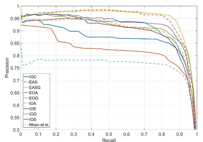
3.8 Precision recall curves computed from different saliency methods . . . 51

3.9 F-Measure computed from different saliency detection methods. . . 52

4.1 Hyperspectral face example . . . 56

4.2 Coordinate systems in 3D space . . . 59

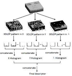
4.3 3D LDP descriptor construction. . . 62

4.4 3D LDP pattern inλdirection at different bands. . . 62

4.5 Implementation details . . . 63

4.6 Examples from the HK-PolyU hyperspectral face dataset . . . 66

4.7 Examples from the CMU hyperspectral face dataset . . . 69

5.1 The Pavia University dataset in tensor representation . . . 76

5.2 Two dimensional representation of the Pavia University dataset . . . 84

5.3 Extended morphological profiles versus tensor morphological profiles . 85 5.4 Examples of two dimensional and three dimensional structural elements. 88 5.5 Classification results using different combinations of cylinder size . . . 90

5.6 Classification maps on the Pavia University dataset . . . 93

5.7 Classification maps on the Pavia Center dataset . . . 94

5.8 Classification maps on the Washington DC dataset . . . 95

6.1 Framework of a supervised hyperspectral image classification system . 98 6.2 False color composite and ground truth labels of hyperspectral datasets 104 6.3 Random sampling on Indian Pines and Pavia University datasets . . . . 105

6.4 Classification maps of the Indian Pines . . . 107

6.5 Overlap between training and testing data on Indian Pines dataset . . . 109

6.6 The overlap region between a single training and testing sample . . . . 109

6.7 Overlap of training and testing data with different size filters . . . 111

6.8 Classification accuracies using a simple mean filter with different sizes 112 6.9 The statistics on the correlation coefficients . . . 118

6.10 Pixel correlations along X dimension . . . 119

6.11 Overlap between the training and testing data . . . 121

6.12 Controlled random sampling strategy on two datasets . . . 123

6.13 Classification accuracies vary with the size of mean filter . . . 125

6.14 Classification accuracies vary with the standard deviation of Gaussian . 127 6.15 Training/classification maps under two sampling strategies . . . 128

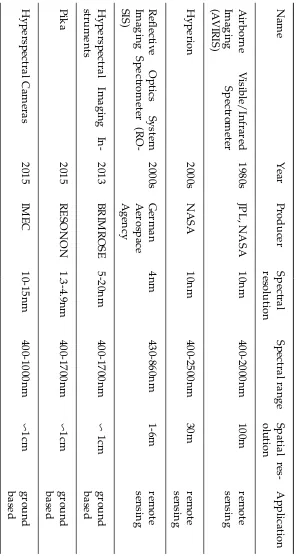
1.1 Hyperspectral imaging instruments . . . 6

2.1 Examples of materials and most useful spectral range for recognition. . 20

2.2 Summary of spectral-spatial feature extraction methods. . . 25

4.1 Recognition rates of different methods on the HK-PolyU dataset . . . . 67

4.2 Recognition rates of different methods on the CMU dataset . . . 69

4.3 Recognition rates of 3D LDP and 2D LDP on two datasets. . . 70

5.1 List of symbols . . . 78

5.3 Classification results on the Pavia University dataset . . . 93

5.4 Classification results on the Pavia Center dataset . . . 94

5.5 Classification results on the Washington DC dataset . . . 95

6.1 Classification results with different features . . . 106

6.2 Classification accuracies on all and non-overlapped testing samples . . 112

6.3 Classification accuracies of different methods when SVM is adopted . . 136

6.4 Classification accuracies of different methods when RF is adopted . . . 137

Introduction

1

.

1

Hyperspectral Imaging

Human vision has evolved to satisfy the requirement of living and played a signif-icant role in finding food or avoiding dangers in the history [1]. We can sense not only the brightness of light but also the color. The trichromatic color vision results from three types of color photoreceptors which are sensitive to three different spectra in the visible light, corresponding to blue, green and red. Via cross-reference of these three colors, we can distinguish a number of color signals. Essentially, color is a vec-tor instead of a scalar and color perception is a comparative sensory phenomenon. However, the human is still restricted to visible light and limited spectral resolution. Researchers have developed different instruments to capture irradiance from ob-jects in various wavelengths. For example, a spectrometer is used to measure the spectral irradiance at a single point, and a conventional RGB camera takes the inte-grated irradiance across the visible wavelength at a region of interest. Different from these two types of instruments, hyperspectral imager can obtain both spatial and spectral information simultaneously. A hyperspectral image usually contains tens or hundreds of continuous light wavelength indexed spectral bands, providing much higher spectral resolution than human vision or regular RGB cameras. The spectrum it covers is not only limited to the visible spectrum but also extends to ultraviolet or infrared light depending on the equipment characteristics. It has been known that objects consisting of different materials may emit, reflect, and absorb light and the proportion is a function of light wavelength or frequency [2]. Therefore, the

ance from objects by a hyperspectral camera can be used as a clue to estimate the physical or chemical properties of the objects.

Due to its high discriminative ability to identify and distinguish different ma-terials, hyperspectral imaging has been widely used in remote sensing to analyze the earth surface for applications such as mining, military, agriculture, environment monitoring, etc. Moreover, with compact and high spatial resolution commercial in-struments being developed, hyperspectral imaging has attracted increasing interests in close-range applications, e.g. food security, biomedicine, biometrics and quality control, etc. Another notable trend in the last decade is the introduction of hyper-spectral imaging into computer vision applications. By providing extra information in the spectral domain, hyperspectral imaging has great potential to push forward research in some challenging problems in computer vision area, such as illumination estimation, super-resolution, camera sensitivity analysis [3, 4], scene analysis [5], document processing [6], object classification [7], etc.

Supporting a broad range of scope in research and applications, hyperspectral image classification covers broad topics in predicting the categories of targets, for instance, general object/scene classification, saliency detection, and image labeling, etc. The targets vary from single pixels, regions, objects to scenes. In remote sens-ing, hyperspectral image classification mainly focuses on pixel-level classification for land-cover classes identification and thematic map generation. In computer vision, hyperspectral images have not been widely used due to absence of large scale image data. Most image classification tasks are still using grayscale or color images which usually contain single object [8, 9, 10].

developed in remote sensing and computer vision during the past decade. Howev-er, most of these methods focus on either pixel-wise spectral information in remote sensing or gray-scale spatial information in computer vision, in accordance with the characteristics of images available in two areas, i.e., high spectral resolution and low spatial resolution in remote sensing, and the opposite in computer vision.

For hyperspectral images obtained by advanced hyperspectral cameras, detailed spectral information and fine spatial resolution enable analysis of both material and structure of objects in a scene. However, most of the existing methods are not suit-able for this task due to the constraints as mentioned above. Therefore, it is necessary to develop new techniques to exploit these underlying spatial and spectral informa-tion in hyperspectral images, thus addressing the limitainforma-tion of human vision, com-puter vision, and remote sensing. Though some attempts have been made in both computer vision and remote sensing recently, there is still a huge gap between hy-perspectral imaging and practical classification applications due to lack of effective spectral-spatial feature extraction methods. This thesis focuses on developing several novel methods based on spatial and spectral analysis, thus facilitating hyperspectral image classification.

1

.

2

Motivation

re-mote sensing image analysis, which usually extract spectral information with band selection or dimensionality reduction without exploring spatial information. Due to random noises from data collection, transmission, and processing, pixel analysis may create pepper and salt like classification map instead of a spatially coherent map [2]. This type of method has ignored the fact that different objects with the same material may be distinguished with the aid of the spatial information.

Nevertheless, facing the challenging obstacles in pattern recognition with compu-tational models, researchers have mainly focused on developing sophisticated feature extraction and machine learning approaches, take two influential works for example, Scale-Invariant Feature Transform (SIFT) [12] and Convolutional Neural Network (C-NN) [9]. These methods are developed to match human vision system by exploring visual processing mechanism in the brain. Although tremendous success has been achieved, most methods are still limited to grayscale or RGB images analysis, mean-ing that there is no additional input into computational models than the human vision system.

Rather than relying on image processing and machining learning algorithms, perspectral imaging provides computer vision with new opportunities. First, hy-perspectral images contain tens or hundreds of bands, thus dramatically increasing its discriminative ability to distinguish a large number of spectral responses beyond the trichromatic human vision system. Furthermore, some extra information beyond visible light range can be captured, for instances, fluorescence which is related to ab-sorption of ultraviolet light, infrared light which can be used to detect plants, and the spectrum in short wave infrared light that water absorbs. The spectral response of materials is called spectral signature, with which the materials can be easily classified or detected.

and classification.

1.2.1 The advance of imaging technology

Hyperspectral imaging instruments were originally developed for airborne and satel-lite platforms so as to measure the spectral characteristics of land cover on earth sur-face. They were seldom available for close-range data collection due to their massive sizes and high prices. With new material, optical, electronics technologies applied to this area, new instruments keep emerging and becoming faster, cheaper, and more compact. Without much loss of spectral range or resolution, the spatial resolution of new hyperspectral cameras has been dramatically increased, making them com-parable to conventional chromatic or monochrome cameras. Table 1.1 shows some examples of hyperspectral imaging instruments developed during the past years. We can observe that there are more and more high spatial and spectral resolution hyperspectral cameras available in the market.

1.2.2 Demand for new hyperspectral image processing methods

For the last decade, a series of methods have been developed to tackle the problems of the particular characteristics of hyperspectral images. Different mathematical for-malisms have been built for typical tasks, such as classification, segmentation, spec-tral mixture analysis. However, most of such works still focus on the specspec-tral domain. With high spatial resolution images available, it is inevitably demanded to develop new spectral-spatial methods for the emerging images. Meanwhile, hyperspectral imaging is still a new topic in the area of computer vision. The limited amount of existing research pays attention to the low level of image processing, for instance, how to obtain the hyperspectral image or videos with high spatial resolution, how to denoise the hyperspectral image and so on. There is a lack of basic methods for the hyperspectral image processing, especially the feature extraction methods.

On the other hand, the hyperspectral imaging has broad application prospects in agriculture, industry, and military due to its higher discriminative ability than conventional cameras. But the lack of basic methods has constrained the analysis in the spectral domain. The various spatial approaches from the computer vision area have not been associated with the spectral methods. A lot of work needs to be done to build the foundation of hyperspectral imaging. It can be expected that there will be a trend that hyperspectral imaging plays a more important role in computer vision and remote sensing in near future, and the spectral-spatial feature extraction will make a difference to the prosperity of hyperspectral imaging.

1.2.3 Challenges

It is a challenging task to extract spectral-spatial features without introducing too much data complexity. The main challenges come from two perspectives: how to fuse spectral and spatial features and how to reduce redundant information in the extracted feature [13]. Several other factors also influence the spectral-spatial feature extraction process, including illumination, noise, and a large amount of data. We summarize these challenging problems as follows:

1. Huge data and high computation complexity. Hyperspectral images consist of tens or hundreds of bands. The size of a single hyperspectral image is usually much bigger than an RGB or grayscale image. To store, process and analyze such massive data is challenging for personal computers.

made of the same material. Due to their different characteristics, there is no straight way to fuse them to represent spectral-spatial features.

3. Curse of Dimensionality. In machine learning, the curse dimensionality refers to a phenomenon that when the dimensionality of feature space increases, the amount of data demanded to obtain a statistically reliable result grows expo-nentially with the dimensionality. This issue is because the number of param-eters to be estimated will increase dramatically. Determining and optimizing such a large number of parameters in a high-dimensional space is problemat-ic. If the number of training instances is much less than the dimension of the features, the learning algorithms tend to overfit. Hyperspectral image classifi-cation usually suffers from such a problem due to its high dimensional nature and limited labeled data. In many cases, the produced spectral-spatial features are of ultra high dimensionality [14, 15].

Figure 1.1: The framework of the proposed methodology.

1

.

3

Objective

1

.

4

Contribution

In this thesis, we have developed three spectral-spatial feature extraction methods for saliency detection, hyperspectral face recognition, and remote sensing image classi-fication. Furthermore, we also discuss the sampling strategy for the evaluation of spectral-spatial methods in remote sensing hyperspectral image classification.

The first method is for salient object detection in hyperspectral images. Object de-tection is an important task for many applications. While most traditional methods are pixel-based on hyperspectral images, many recent efforts have been putting on extracting spectral-spatial features. In this method, we extend Itti’s visual saliency model to the spectral domain and introduce the spectral-spatial distribution based saliency model for object detection. This model enables the extraction of salient spec-tral features in the scale space, which is related to the material property and spatial layout of objects. To our knowledge, this is the first attempt to combine hyperspec-tral data with salient object detection. Several methods have been implemented and compared to show how color component in the traditional saliency model can be replaced by spectral information.

recognition methods, our method can describe the distinctive micro-patterns which integrate both spatial and spectral information in faces.

The third approach is based on morphological profiles for remote hyperspectral image classification. Traditional mathematical morphology operations are limited to extracting spatial feature in two-dimensional data and are not able to be applied to hyperspectral image due to the so-called ordering problem. In this approach, we pro-pose a novel multi-dimensional morphology descriptor, namely, tensor morphology profile (TMP). TMP is a general framework to extract multi-dimensional structures in high-dimensional data. Thenth-order morphology profile is proposed to work with thenth-order tensor, which can capture the inner high order structures. By treating a hyperspectral image as a tensor, it is possible to extend morphology operations to high dimensional data so that this powerful tool can be used to analyze hyperspectral images with fused spectral-spatial information.

al-gorithms because it ’s hard to determine whether the improvement of classification accuracy is caused by incorporating spatial information into a classifier or by increas-ing the overlap between trainincreas-ing and testincreas-ing samples. To partially solve this problem, we propose a novel controlled random sampling strategy for spectral-spatial meth-ods. It can substantially reduce the overlap between training and testing samples and provides more objective and accurate evaluation.

1

.

5

Thesis Outline

1

.

6

List of Publications

1. Jie Liang, Jun Zhou, Yuntao Qian, Lian Wen, Xiao Bai, and Yongsheng Gao. On the sampling strategy for evaluation of spectral-spatial methods in hyperspectral image classification.IEEE Transactions on Geoscience and Remote Sensing, PP(99):1– 19, Nov 2016. (Corresponding to Chapter 6).

2. Jie Liang, Jun Zhou, Yuntao Qian, and Yongsheng Gao. Tensor morphology pro-file versus extended morphology propro-file: hyperspectral image classification with spatial-spectral descriptor. Submitted to IEEE Journal of Selected Topics in Applied Earth Observations and Remote Sensing, Aug 2016. (Corresponding to Chapter 5).

3. Changhong Liu, Jun Zhou, Jie Liang, Yuntao Qian, Hanxi Li, and Yongsheng Gao. Exploring structural consistency in graph regularized joint spectral-spatial sparse coding for hyperspectral image classification.IEEE Journal of Selected Topics in Applied Earth Observations and Remote Sensing, PP(99):1–14, Aug 2016.

4. Jie Liang, Jun Zhou, Xiao Bai, and Yuntao Qian. Salient object detection in hyper-spectral imagery. In2013 IEEE International Conference on Image Processing, pages 2393–2397. IEEE, Sep 2013. (Corresponding to Chapter 3).

5. Jie Liang, Ali Zia, Jun Zhou, and Xavier Sirault. 3D plant modelling via hyper-spectral imaging. In IEEE International Conference on Computer Vision 2013 and Computer Vision for Accelerated Bioscience, pages 172–177. IEEE, Dec 2013.

6. Jie Liang, Jun Zhou, and Yongsheng Gao. 3D local derivative pattern for hyper-spectral face recognition. In2015 11th IEEE International Conference and Workshops on Automatic Face and Gesture Recognition, volume 1, pages 1–6. IEEE, May 2015. (Corresponding to Chapter 4).

8. Jun Zhou, Jie Liang, Yuntao Qian, Yongsheng Gao, and Lei Tong. On the sam-pling strategies for evaluation of joint spectral-spatial information based classi-fiers. In 7th Workshop on Hyperspectral Image and Signal Processing: Evolution in Remote Sensing, 2015.

9. Ali Zia, Jie Liang, Jun Zhou, and Yongsheng Gao. 3D reconstruction from hyper-spectral images. In2015 IEEE Winter Conference on Applications of Computer Vision, pages 318–325. IEEE, Jan 2015.

Literature Review

2

.

1

Hyperspectral Imaging Technology

Before introducing hyperspectral imaging in more details, this section explains the terminology commonly used in related areas, for example, hyperspectral imager, hyperspectral imaging, multispectral imaging, spectral imaging, spectrometer, spec-troscopy, and photography.

A hyperspectral imager is an instrument which can capture hyperspectral data/im-ages, while hyperspectral imaging refers to the complete hyperspectral data pro-cessing including collection, measurement, analysis and interpretation of spectra. Both hyperspectral imaging and multispectral imaging are kinds of spectral imaging which capture the spectral information at every pixel on the image plane. The differ-ence is that the former emphasizes high spectral resolution and continuous spectral range, while the latter contains only several bands without spectral continuity re-quirement. Spectral imaging is a combination of photography and spectroscopy. While photography projects scene and object on an electronic sensor or photograph-ic film, spectroscopy studies the interaction between matter and radiated energy at a single point. Spectral imaging takes advantage of both photography and spec-troscopy and captures both spatial and spectral information in a scene. Although the conventional camera can capture partial spectral information by separating light into three channels dominated by red, green and blue, the spectral resolution is rough and cannot cover spectrum out of the visible range compared to hyperspectral imag-ing. For the sake of conciseness and without confusion, we use "spectral imaging",

Figure 2.1: Brimrose hyperspectral imaging system.

"hyperspectral imaging" and "multispectral" interchangeably in the rest of the thesis.

The concept of hyperspectral imaging can trace back to 1980s when NASA’s Jet Propulsion Laboratory developed a new remote sensing instrument AVIRIS which covers the wavelengths from 0.4 to 2.5 µm and produces more than two hundred

scan-ning systems. On the contrary, snapshot cameras are more suitable for close-range computer vision applications where the complete spatial layout of objects and scenes shall be taken at a time. In Fig. 2.1, we show a Brimrose hyperspectral imaging system in the Spectral Lab at Griffith University.

Compared with conventional cameras, hyperspectral cameras have their limita-tions. First, the spatial resolution of images is relatively low at the cost of extra spectral bands. Furthermore, the imaging process is time-consuming, generally re-quiring the scene remain still during the exposure time which can last for several or tens of seconds. The exposure time is closely related to illumination condition. Since incident light is separated into narrow bands, a limited amount of light arrives at the sensor. Therefore, the generated images may have low signal to noise ratio. This can only be solved by either extending the exposure time or increase the light intensity when a sensor is given. Sometimes the band images may suffer from out of focus problem as the focus is normally tuned on a single band.

During the past several years, new hyperspectral imaging technologies have been developed so as to allow fast snapshot mechanism. For example, IMEC has designed a new series of hyperspectral cameras with snapshot mosaic technology1_{. The new}

camera is developed based on a large CMOS sensor wafer in which different pix-els in an array are sensitive to different wavelengths. Therefore, this camera can capture real-time images and videos as traditional digital cameras, but with many more spectral channels. This advantage has dramatically increased the feasibility of hyperspectral cameras in real-world computer vision applications.

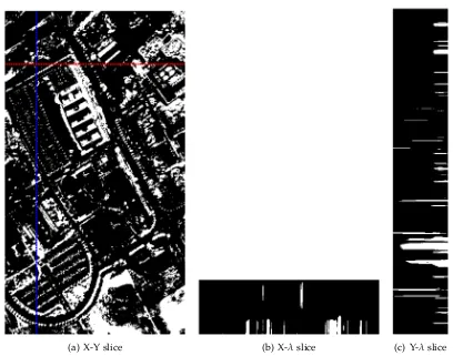
When data representation is concerned, a hyperspectral image is usually in the form of a data cube as shown in Fig. 2.2. It consists of two spatial dimensionsXand

Y, and a spectral dimension λ. Each pixel is a vector corresponding to the spectral

response at the spatial location. At each wavelength, a grayscale band image can be acquired, representing the spatial distribution of the scene at this band.

1_{Products link: http://www2.imec.be/be_en/research/image-sensors-and-vision-systems/}

Figure 2.2: Representation of a hyperspectral image and meaning in different dimen-sions2.

2

.

2

Radiometry for Hyperspectral Imaging

There has been a long history since researchers began to study the light and its in-teraction with matter. Radiometry is such a tool to measure light in the magnetic spectrum. The target of radiometry research covers different light sources such as sunshine and man-made lights, objects of different scales from man-made to earth and universe, and a variety of imaging devices including naked eyes, spectrome-ter, cameras and radio telescope. Among various imaging devices, spectrometers and cameras are particularly useful to measure the interactions of objects and light courses. Light contains abundant spectral information related to electromagnetic ra-diance. Imaging devices normally cover ultraviolet, visible and infrared light in the spectral range. Ultraviolet can be further divided into UVA, UVB, and UVC. Visible light is the spectral range which human vision can perceive. Infrared light covers near-infrared, short wave infrared, middle wave infrared, and long wave infrared light spectra. Different spectral ranges of light have unique characteristics and serve different functions. Fig. 2.3 shows the electromagnetic spectrum with respect to the

2_{This figure is from http://www.bodkindesign.com/products-page/hyperspectral-imaging/}

Figure 2.3: Electromagnetic spectrum3.

wavelength.

Like the formation of normal images, hyperspectral imaging captures a propor-tion of spectrum within the electromagnetic spectrum. While a color image is nor-mally formed by integration of light in red, blue, and green wavelengths, hyper-spectral imaging is able to cover up to hundreds of bands in ultraviolet, visible and infrared ranges.

2.2.1 Spectral range, absorption, and materials

In physics, when an object interacts with light, it may absorb the incident radiation over a range of frequencies which is referred as spectrum absorption. It is primarily determined by the atomic and molecular composition of the material. Consequently, this property can be used to distinguish different elements and plays an important role in astronomy. For instance, each element has its own spectral atom spectrum. When scaling up, the molecule spectrum and material have photophysical effect. Different materials have distinct absorption properties. The wider range and higher resolution of the spectra a sensor can cover, the more materials it can distinguish [2, 16]. Across the whole electromagnetic spectrum, the visible bands only occupy a small proportion and a large amount information existing in other bands.

A lot of physical phenomena are connected with spectral reflectance or absorp-tion. Plants, water/moisture, and DNA all have their own spectral signatures. In Table 2.1, we show some examples of materials which can be distinguished with specific spectral range.

Table 2.1: Examples of materials and most useful spectral range for recognition.

Materials Spectral Range

Chlorophyll absorbtion/vegetation reflectance 510-970 nm

Oxygenation in blood 500-900 nm

Hydrocarbon organic compounds 750-950 nm

Water absorption 970, 1450,1850 nm

PVC/plastic recycling 1700-1900 nm

Minerals mapping 2300-2400 nm

CH4 2300 nm

CO2 2100,3500,4800 nm

2

.

3

Feature Extraction in Computer Vision and Remote

Sens-ing

visual words [21]. Theoretically, a feature is a pattern which represents particular property of an image and sometimes even a robust presentation of image. In this chapter, I review some local features, texture features and color features that are relevant to my research, as well as how they are extracted and described.

2.3.1 Local image feature

Local features are an important cue to predict the shape of an object [17]. Other causes include sharp changes in albedo, surface orientation or illumination. Local features are very useful because it reflects the properties of images: the change of albedo results from the texture variant; the change of surface orientation shows the shape; the illumination change is caused by the movement of light source.

Local features can be extracted at points, edges or small patches in an image. Be-sides their locations, details about the regions where features locate can form descrip-tors for other computer vision steps. Depending on the properties of local feature and their corresponding patterns in images, local features can be used in various ways. For example, they may represent specific objects in some applications, such as road recognition which can be implemented by line detection in an image [22], and impu-rity identification in quality inspection of glasses by detecting blobs. Local features could also possess transform invariant property, which is one of the foundations of image registration. Last, a class of objects or images need general representation for recognition and classification purposes. A set of features can play such a role and act as abstract description.

2.3.2 Texture feature

from texture [17]. The reason why texture is important is that it describes prop-erty of materials and helps to identify an object. Although traditionally extracted from grayscale and color images, texture can be associated with spectral information which is covered in this thesis.

In order to represent a local texture, two factors shall be addressed: what texture element shall be extracted and how texture is distributed. An element of texture is usually called texton. Textures vary a lot so it is difficult to predict which textons exist in an image. A solution to this problem is to split textures into subelements like spots and bars. Then subelements are detected by applying a set of filters at various scales to an image so that each of subelement is represented by the vector of the corresponding filter. At last, the summary of the output maps provides a representation of texture in the image.

2.3.3 Color feature

Color is a kind of low spectral resolution information located in red, green and blue bands, which can be used for illumination estimation, saliency detection, image segmentation, specularity and shadow removal, etc. There are several color spaces, i.e. RGB color space, CIE XYZ color space, HSV color space. Each of them represents different information and can be used in various applications. However, color itself is not capable of distinguishing different materials due to metamerism [23], i.e., the same color may correspond to different spectral power distribution.

Figure 2.4: Vegetation, soil and water spectra recorded by AVIRIS [11].

the color histogram [24] which is a good color feature descriptor.

2.3.4 Spectral feature extraction in remote sensing

In remote sensing, researchers focus more on the spectral domain. It is because that, on one hand, the hyperspectral images consist of tens or hundreds of wavelength in-dexed bands which contain rich information of spectra; on the other hand, the spatial resolution of remote sensing image is quite low, usually measured by meters. As a result, researchers need to unmix a single pixel (which is to analyze the components of a pixel) to different components for image analysis, rather than considering shapes or textures in an image. Note that a pixel with a spectral vector is a feature itself. Therefore, most algorithms in this area are pixel based. The problem for feature ex-traction becomes how to use the feature efficiently rather than how to represent the feature. In order to solve this problem, a lot of research has been done in feature selection and feature extraction, including methods that are supervised and unsu-pervised, parametric and nonparametric, linear and nonlinear [25]. All of them try to seek the informative subspace of features.

useful. Every material has its unique spectral absorption feature. However, discrimi-native information might only exist in a portion of wavelengths. For example, Fig. 2.4 shows that the difference of spectra between vegetation and soil mainly lies in the visible range but not the far infrared range. Even if the spectral reflectance is not sim-ilar, the spectral information may be redundant considering that many contiguous bands are highly correlated. Moreover, noises coming from imaging environment and instruments often contaminate some bands. Therefore, the raw hyperspectral bands shall be preprocessed for remote sensing applications. For the hyperspectral images captured on the ground as used in my research, this problem also needs to be considered.

A simple but useful method for dimensionality reduction is principal component analyze (PCA) [26]. Based on statistics of data, its objective is to find the most vari-ant dimensions of data and map the original data on these dimensions so that the variance of data is maximally retained. Mathematically, given the original feature set

Xand its element xi, each new featureyi is calculated using the following equation:

yi =wTxi (2.1)

where the columns ofware the eigenvectors of the covariance matrix of the original feature setX. The method to calculate the covariance matrix is shown in Equation 2.2 whereµis the mean vector ofX.

C= 1

N

∑

T_(x

j−µj) (2.2)

classes [27].

2

.

4

Spectral-spatial Feature Extraction

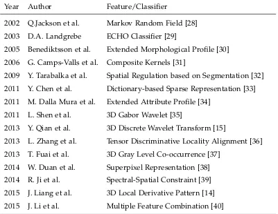
Table 2.2: Summary of spectral-spatial feature extraction methods.

Year Author Feature/Classifier

2002 Q.Jackson et al. Markov Random Field [28] 2003 D.A. Landgrebe ECHO Classifier [29]

2005 Benediktsson et al. Extended Morphological Profile [30] 2006 G. Camps-Valls et al. Composite Kernels [31]

2009 Y. Tarabalka et al. Spatial Regulation based on Segmentation [32] 2011 Y. Chen et al. Dictionary-based Sparse Representation [33] 2011 M. Dalla Mura et al. Extended Attribute Profile [34]

2011 L. Shen et al. 3D Gabor Wavelet [35]

2013 Y. Qian et al. 3D Discrete Wavelet Transform [15]

2013 L. Zhang et al. Tensor Discriminative Locality Alignment [36] 2013 T. Fuai et al. 3D Gray Level Co-occurrence [37]

2014 W. Duan et al. Superpixel Representation [38] 2014 R. Ji et al. Spectral-Spatial Constraint [39] 2015 J. Liang et al. 3D Local Derivative Pattern [14] 2015 J. Li et al. Multiple Feature Combination [40]

under both sunlight and halogen light, but color is not. Due to its high spectral resolution, hyperspectral images provide much more information than color image, and its inner constraints can help to estimate the reflectance, therefore making them particularly useful for computer vision tasks [16].

The spatial information in a hyperspectral image may cover many factors. These include local information such as structures, textures, and contextual information, as well as global information such as geometric information. Due to the high di-mensionality of this kind of feature, it is quite expensive to associate both spatial and spectral features at the same time. So an alternate way is to consider them separately.

The advantage of using hyperspectral data in land cover classification is that spectral responses reflect the properties of components on the ground surface [2]. Therefore, raw spectral responses can be used directly as the discriminative features of different land covers. At the same time, hyperspectral data also possesses the ba-sic characteristic of conventional images - the spatial information which corresponds to where a pixel locates in the image. The spatial information can be represented in different forms, such as structural information including the size and shape of object-s, textures which describe the granularity and patternobject-s, and contextual information which can express the inter-pixel dependency [41]. This is also the foundation of developing spectral-spatial methods for hyperspectral image classification.

to their spectral responses [43, 41]. Similar information is explored in image segmen-tation which groups spatially neighboring pixels into clusters based on their spectral distribution [44, 45].

Secondly, common usage of joint spectral-spatial information lies in the feature extraction stage. While traditional spectral features are extracted as responses at single pixel level in hyperspectral images, spectral-spatial feature extraction meth-ods use spatial neighborhood to calculate features. Typical examples include tex-ture featex-tures such as 3D discrete wavelet [15], 3D Gabor wavelet [46], 3D scattering wavelet[47], and local binary patterns [48]. Morphological profiles, alternatively, use closing, opening, and geodesic operators to enhance the spatial structures of object-s [30, 49, 34]. Other object-spectral-object-spatial featureobject-s include object-spectral object-saliency [50], object-spherical harmonics [51], and affine invariant descriptors [52]. Heterogeneous features can be fused using feature selection or reduction approaches [25].

Thirdly, some image classification approaches rely on spatial relation between pixels for model building. A direct way of doing so is calculating the similarity be-tween a pixel and its surrounding pixels [53]. Markov random field, for example, treats hyperspectral image as dependent data and uses spectral information in the local neighborhood to help pixel class prediction [54, 45, 55]. Similar spatial struc-tures are explored in conditional random fields [56], hypergraph modelling [39], and multi-scale analysis [57]. The spatial information can also be explored in constructing composite kernels in support vector machines [31]. Supervised learning approaches, such as K-nearest neighbors, linear discriminant analysis, Bayesian analysis, support vector machines, etc. are widely used in these classification tasks [58, 59]. Nonethe-less, some approaches adopt semi-supervised or active learning strategies [60, 61].

2.4.1 Extended morphological profiles

cannot be applied to hyperspectral images directly since there is no explicit ordering relationship in vectors. In other words, neither maximum nor minimum, which are necessary for basic morphological operations, is not defined for a set of vectors.

The details of this method and its variation can be found in a survey paper from Fauvel et al [41]. The spatial feature is extracted as follows

Ω(n)

(I) =ho(n)(I), ...,o(1)(I),I,c(1)(I), ...,c(n)(I)i (2.3) where o(n)_{(I) andc}(n)_{(I)are the opening and closing operations with a disk-shape} structural element of size n, respectively. As different sizes of structuring elements are used, the morphological profile Ω(n)(I) is capable of integrating multi-scale in-formation. Before the feature extraction, a principle component analysis (PCA) step is applied to hyperspectral images to reduce the dimension of the data. Then the morphological profiles are obtained on each of themprimary components:

ˆ

Ω(n)

m (I) =

h

Ω(n)

1 (I),Ω

(n)

2 (I), ...,Ω

(n)

m (I)

i

(2.4)

In the last step, the morphological profiles are stacked with the spectral response to form the spectral-spatial feature.

2.4.2 3D Gabor wavelet

Three dimensional Gabor filter [35] is the extension of two dimensional Gabor which is widely adopted in texture feature extraction. By tuning the scale and orientation, the Gabor Wavelet can extract multi-scale and multi-orientation features from images. A 3D Gabor filter with the frequency f and orientation (φ,θ) can be defined as

following

Gf,φ,θ(x,y,b) =N×exp(−(

x0

σx

2

) + (y

0

σy

2

) + (b

0

σb

2

This function is a Gaussian kernel function modulated by a sinusoid plane wave. N is the normalise factor. [x0,y0,b0]T _{is transformed signal which is coincide with}

orientation of the sinusoid. It can be calculated as

[x0,y0,b0]T = R×[x−xc,y−yc,b−bc]T (2.6)

where(xc,yc,bc)is the central position for signals and R is the rotation matrix defined

by(φ,θ). σx,σyandσbare width of Gaussian envelop in different axis. Regarding the

sinusoid plane wave,wis the axis of the wave vector and u−v is the perpendicular plane in frequency domain. u= fsinφcosθ,v= fsinφsinθ,w= fcosφ.

2.4.3 3D discrete wavelet transform

The three-dimensional wavelet texture features proposed by Qian et al [15] is a re-al 3D feature on hyperspectrre-al images. In this method, hyperspectrre-al data cube is treated as a a whole tensor and it is composed at different scales, frequencies and ori-entations by the 3D discrete wavelet transform. The definition of continuous wavelet transform is

Ψψ

x(τ,s) =

Z

x(t)·ψτ,s(t)dt (2.7) where ψτ,s is the basis functions (wavelet) with s and τ controlling the scale and translation, respectively. x(t) is the original signal in the time domain. When it comes to discrete samples, discrete wavelet transform (DWT) is implemented by a series of filters in the frequency domain. Since hyperspectral images consist of three dimensions, 3D-DWT exploits the correlation along the wavelength axis, as well as along the spatial axes, so that both spatial and spectral structures of hyperspectral images can be adequately mapped into the extracted features.

levels of decomposition, the original data is separated into 15 sub-cubesC1,C2, ...,C15

based on the bandwidth, such that each of the sub-cubes contains different scales of information. To further capture the spatial distribution of hyperspectral images, a mean filter is applied on the sub-cubes:

ˆ

Cn(x,y, .) =

1 9

x+1

∑

i=x−1

y+1

∑

j=y−1

C(i,j, .) (2.8)

where C(i,j, .) is the spectral response at the position of (i,j). [x−1,x+1] and

[y−1,y+1]define a 3 by 3 neighbourhood.

In order to keep the sub-cube and the original data cube at the same size, the filtered signals are not down-sampled as what the traditional DWT does. Then these sub-cubes are concatenated into the wavelet features. The multidimensional function is carried out along two spatial dimensionsxandy, as well as the spectral dimension

λ, respectively. The final concatenation work as the feature for the whole data cube

and can be represented as:

f(x,y) = (Cˆ₁x, ˆC₂x, ..., ˆC₁₅x, ˆC₁y, ˆC₂y, ..., ˆCy₁₅, ˆCλ

1, ˆCλ2, ..., ˆC15λ) (2.9)

where f(x,y)is the 3D-DWT feature at location (x,y).

2.4.4 Tensor modeling

be arranged as a three-dimensional array with the modes corresponding to spatialx

spatialyand wavelengthλ. Zhang et al. [36] represented the spectral-spatial feature

of a pixel as a tensor. The feature was constructed by the spectra of the pixel itself as well as its k nearest neighbors. Then a tensor discriminative locality alignment (TD-LA) was developed to transform the high-order tensor space to a low dimensional feature space via patch optimization which included the information of same and different classes in the training data. Its superiority over several unsupervised and supervised feature dimension reduction methods was proved on three commonly used hyperspectral datasets. Meanwhile, Velasco-Forero et al. [63] developed an ad-ditive morphological decomposition (AMD) which decomposed an image into two parts. While the first part was formulated by the summation of anti-extensive trans-formations and extensive transtrans-formations, representing all contrast and boundary information, the second part was related to the residue of anti-extensive transfor-mations and extensive transfortransfor-mations with different scales, constituting a hierarchy of multiscale texture components. Then tensor modeling methods were employed to reduce the dimension of extracted features in which the spatial information was maintained.

2.4.5 Other spectral-spatial operations

Figure 2.5: Tensor structure in different formats. From left to right: cube, fibers, slices (modified from [62]).

algorithms, major voting can be used to reassign the labels of pixel wise classification by counting the most frequent labels in the region so as to create a smooth classifi-cation map. Although this method is simple and straightforward to associate the spatial information with spectral information for hyperspectral image classification, the classification results heavily depend on the segmentation algorithms.

equivalent to the minimization of the energy functionU(Y|X).

2

.

5

Classification Methods

Effective and efficient classifiers are very important for hyperspectral image classifi-cation. The inputs to classifiers are normally extracted features or image representa-tion. Depending on the availability of the labeled data, classification methods can be categorized into unsupervised learning and supervised learning. Unsupervised clas-sification methods can be used to discover groups of similar samples in the dataset based on statistics. Clustering is a typical unsupervised classification method. The most popular clustering algorithm is K-means clustering [66]. It adopts an iterative updating methods to partition data samples intok clusters in order to minimize the within class distance. On the contrary, supervised learning methods use labeled da-ta to train a classifier and then apply it to unseen dada-ta. It is usually more reliable than unsupervised methods. In this thesis, we mainly focus on supervised learning methods.

For hyperspectral image classification, there are only limited labeled data avail-able for training and testing due to lacking of benchmark datasets and high cost of ground truth data collection. Therefore, not all of supervised learning methods are suitable for such task, especially those require a large amount of training data such as deep learning approaches. We briefly introduce three typical methods commonly used in hyperspectral image classification: support vector machine, random forest, and extreme learning machine.

2.5.1 Support vector machine

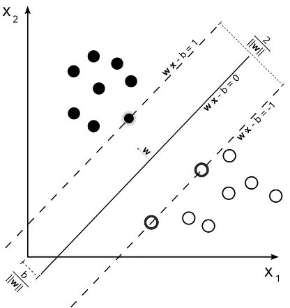
Support vector machines (SVM) has been widely used in classification tasks [67]. It aims at estimating a hyperplane(s) to classify data into two classes such that the maximum margin between the hyperplane and training samples is achieved. The

Figure 2.6: Maximum-margin hyperplane for a two-class SVM. White and black dots represent sample from class "+1" and "-1", respectively4.

periority of SVM over the old statistical learning method is that it introduces the con-cept of geometrical margin that involves only a few training samples at the bound-aries (support vectors), which makes it very suitable to deal with small training set problem. Fig. 2.6 shows an example to explain this concept. Given a binary clas-sification problem in two-dimensional feature space X1 and X2. There are samples

represented as white and black dots from class "+1" and "-1", respectively. In order to fully separate two classes, the optimal hyperplane should find those training samples near boundaries and maximize the distances between them and hyperplane. If the hyperplane can be defined asw·x−b=0, then the total distance equals to _kw2_k.

Mathematically, the optimal hyperplane can be solved by the following linearly constrained optimization problem:

Minimize

w, ξ 1 2w

T_w+C

∑

ξi

Subject to yi(wTφ(xi) +b≥1−ξi)

ξi ≥0

whereξ is slack variables introduced to account for the nonseparability of data, and

the constant C is a regularization parameter which controls the penalty assigned to errors. For the linear non-separable problem, φ(xi) is a kernel function, mapping

data into a high dimensional space. The kernels can be polynomial, Gaussian radial basis function, and sigmoid function. A widely used Matlab toolbox for classification can be found at [68].

2.5.2 Random forest

Algorithm 1Random forest algorithm

Require: Training set, the number of trees k, the number of features m

Randomly sample a subset Sof training setNtimes foreach subsetSi in N do

Build a decision treeT

foreach nodenin Tdo

Randomly selectmfeatures and split the tree Stop until the tree is fully grown and not pruned end for

end for

Combine allktrees by major voting to construct the classifier

Random forest is an ensemble learning method that combines multiple decision trees to construct more powerful classifier than any individual tree [69]. It has drawn increasing interest in hyperspectral image classification [70, 71, 72]. The advantage of this method is that it can avoid the overfitting problem even if the feature dimension is high. Unlike conventional decision trees which may overfit the training dataset, random forest uses multiple subsets of the training data and build multiple deci-sion trees, thus to avoid the correlation of multiple trees. Furthermore, instead of using all feature variables, it only uses some of the features when splitting the trees. The algorithm is fast to implement and can deal with large-scale datasets with high dimension variables.

data is drawn from training set with replacement. A decision tree is learned from each subset. In each split of the procedure, only m randomly selected variables are considered. The iteration stops when the tree is fully grown. The output is an ensemble tree which is used to make prediction for new data.

2.5.3 Extreme learning machines

In recent years, neural network methods, especially deep learning, regain prosperity in the machine learning community. Huang et al [73] proposed extreme learning machine (ELM) which is a two-layer feedforward neural network that provides ex-cellent classification performance without long training time. The characteristics of ELM make it qualified for the hyperspectral image classification in which only a limited training data are available, but massive data needs to be processed [38, 48].

Salient Object Detection in

Hyperspectral Imagery

3

.

1

Introduction

A hyperspectral image consists of tens or hundreds of contiguous narrow spectral bands. Each pixel in a hyperspectral image is a vector of spectral responses across the electromagnetic spectrum (normally in the visible to the near-infrared range). Such spectral responses are related to the material of objects in a scene that has been imaged, which provides valuable information for automatic object detection.

Due to its high dimensionality, traditional pattern recognition and computer vi-sion technology cannot be directly applied to hyperspectral imagery. Most object detection methods for hyperspectral images are still pixel-based, i.e., performing pixel-wise detection and classification based on spectral signatures followed by post-processing to group pixels or segment regions from an image [7, 44]. In this manner, feature extraction is only performed in the spectral domain, but the spatial distribu-tion of objects has not been fully explored. More recently, researchers have tried to use spectral-spatial structure modeling for hyperspectral image classification. Such efforts include Markov random field and conditional random field [56, 45], which introduces spatial information into classification steps using a probabilistic discrimi-native function with contextual correlation. Furthermore, multi-scale time-frequency signal analysis methods based on 3D discrete wavelet transform have also been

troduced for object detection and classification in remote sensing imagery [15].

Visual saliency is another type of approaches to extract multi-scale image features. The concept of saliency is from human attention model, which detects objects or regions in a scene that stand out with respect to their neighborhood [75]. As a consequence, saliency detection models are normally established on the trichromatic or greyscale images, which are visible to human eyes. When used for object detection in computer vision and robotics applications, saliency map is often constructed in a bottom-up manner. For example, Itti et al. calculated multi-scale differences of intensity, color, and orientation features, and linearly combined them to form the final saliency map [76]. Liu et al. formulated the saliency detection problem as a region of interest segmentation task [77]. Salient features were extracted at the local, regional and global levels, and were combined via learning with conditional random field. Similarly, many saliency detection methods try to detect image regions that are different from its neighborhood in the scale space, as reviewed in [75].

When applied to hyperspectral imagery, saliency model has been used for image visualization. Wilson et al. employed contrast sensitivity saliency to fuse different bands of hyperspectral remote sensing images so that it can be used for visual anal-ysis [78]. Itti’s model [76] has been combined with dimensionality reduction method to convert a hyperspectral image to a trichromatic image that can be displayed on computer screen [79]. Saliency has also been used to help edge detection and to predict eye fixation on hyperspectral images [80, 81].

hy-Figure 3.1: The architecture of Itti’s saliency model [76].

perspectral image into an RGB image and applies Itti’s model directly. The second method replaces the color double-opponent component with grouped band compo-nent. The third method directly uses the raw spectral signature to replace the color component. The last method creates a spectral-spatial distribution and uses it for saliency prediction.

3

.

2

Itti’s Saliency Model

The saliency detection method proposed by Itti et al. mimics the behavior and structure of the early primate visual system [76]. It extracts three types of multi-scale features, including intensity, color, and orientation, and then computes their center-surround differences. These differences are linearly combined to form the final saliency map.

of visual cues are then extracted from the intensity, color, and orientation features and each of them forms a conspicuity map. The intensity feature is obtained by av-eraging the RGB channel values at each pixel. By calculating the differences between each pair of fine and coarse scales, six intensity channels are generated. The second set of features are calculated from a set of color opponency between red, green and blue values against yellow value at each pixel. Center-surround differences for each pair of color opponent are then derived over three scales, which leads to 12 channels. The orientation features are generated using a set of even-symmetric Gabor filters. The dominant orientation at each pixel is recovered, whose center-surround differ-ences are calculated at six scales and four orientations. This leads to 24 orientation channels. Channels of each type are then linearly combined to form three conspicu-ity maps in terms of the intensconspicu-ity, color and orientation. Finally, the mean of the conspicuity maps becomes the saliency map.

3

.

3

Saliency Extraction in Hyperspectral Images

3.3.1 Spectral saliency

3.3.1.1 Hyperspectral to trichromatic conversion

What has hindered the adoption of saliency extraction by hyperspectral object de-tection is the large amount of bands in the spectral data. This makes the color component not able to be calculated directly. Furthermore, effective extraction of the intensity and texture saliency requires a grayscale image to be used. A direct solution to this problem is conversion of a hyperspectral image into a trichromat-ic image, whtrichromat-ich allows traditional saliency model to be appltrichromat-icable. As pointed out in [79], this can be achieved by dimensionality reduction, band selection, or color matching functions.

I(λi)for each of the bandsλi, such conversion can be implemented by the following

color matching function:

It = N

∑

i=1

I(λi)Wt(λi) (3.1)

where N is the total number of bands, t = {X,Y,Z} are the tristimulus component of the color space, andWt comes from the spectral sensitivity curves of three linear

light detectors that yield the CIE XYZ tristimulus valuesX,Y, andZ. This conversion is then followed by a further transform step to the sRGB color space [83], then Itti’s method can be applied.

Figure 3.2: Spectral band group.

3.3.1.2 Spectral band opponent

Although the above method is straightforward, it does not take advantage of the high spectral resolution information provided by the hyperspectral image. Notice that the second conspicuity map in Itti’s method is formed from RGB color channels, we shall be able to replace the color opponents with groups spectral bands that are approx-imately correspondence to these color channels. Furthermore, the yellow channel in Itti’s method is extracted from RGB channel. For a hyperspectral image, we can group spectral bands to represent the original multichannel color information. To do so, we divide the bands into four groups with each group occupying approxi-mately the same width of visible spectrum, as shown in Fig. 3.2. Then the original single value color component is replaced by a vector, so the double opponency can be computed as follows