This is a repository copy of
Model structure detection and system identification of metal
rubber devices
.
White Rose Research Online URL for this paper:
http://eprints.whiterose.ac.uk/74663/
Monograph:
Zhang, B., Lang, Z.Q., Billings, S.A. et al. (2 more authors) (2010) Model structure
detection and system identification of metal rubber devices. Research Report. ACSE
Research Report no. 1012 . Automatic Control and Systems Engineering, University of
Sheffield
[email protected] https://eprints.whiterose.ac.uk/ Reuse
Unless indicated otherwise, fulltext items are protected by copyright with all rights reserved. The copyright exception in section 29 of the Copyright, Designs and Patents Act 1988 allows the making of a single copy solely for the purpose of non-commercial research or private study within the limits of fair dealing. The publisher or other rights-holder may allow further reproduction and re-use of this version - refer to the White Rose Research Online record for this item. Where records identify the publisher as the copyright holder, users can verify any specific terms of use on the publisher’s website.
Takedown
If you consider content in White Rose Research Online to be in breach of UK law, please notify us by
Model Structure Detection and System Identification of Metal
Rubber Devices
B. Zhang, Z. Q. Lang, S. A. Billings, G. R. Tomlinson, and J. A. Rongong
Research Report No.1012
Department of Automatic Control and Systems Engineering The University of Sheffield
Mappin Street, Sheffield, S1 3JD, UK
Jun 2010
Model Structure Detection and System Identification of
Metal Rubber Devices
B. Zhang
a, Z.Q. Lang
a, S. A. Billings
a, G. R. Tomlinson
b, and J. A. Rongong
baDepartment of Automatic Control and Systems Engineering, The University of Sheffield, Mappin Street, Sheffield S1 3JD, UK bDepartment of Mechanical Engineering, The University of Sheffield, Mappin Street, Sheffield S1 3JD, UK
E-mail: {b.zhang, z.lang, s.billings, g.tomlinson, j.a.rongong}@sheffield.ac.uk
Abstract
Metal rubber (MR) devices, a new wire mesh material, have been extensively used in recent years due to several unique properties especially in adverse environments. Although many practical studies have been completed, the related theoretical research on metal rubber is still in its infancy. In this paper, a semi-constitutive dynamic model that involves nonlinear elastic stiffness, nonlinear viscous damping and bilinear hysteresis Coulomb damping is adopted to model MR devices. After approximating the bilinear hysteresis damping using Chebyshev polynomials of the first kind, a very efficient procedure based on the orthogonal least squares (OLS) algorithm and the adjustable prediction error sum of squares (APRESS) criterion is proposed for model structure detection and parameter estimation of an MR device for the first time. The OLS algorithm provides a powerful tool to effectively select the significant model terms step by step, one at a time, by orthogonalizing the associated terms and maximizing the error reduction ratio, in a forward stepwise procedure. The APRESS statistic regularizes the OLS algorithm to facilitate the determination of the optimal number of model terms that should be included into the dynamic model. Because of the orthogonal property of the OLS algorithm, the approach leads to a parsimonious model. Numerical ill-conditioning problems confronted by the conventional least squares algorithm can also be avoided by the new approach. Finally by utilising the transient response of a MR specimen, it is shown how the model structure can be detected in a practical application. The identified model agrees with the experimental measurements very well.
Keywords: metal rubber; nonlinear damping material; nonlinear system identification; bilinear hysteresis model
1. Introduction
Metal rubber (MR) devices[1], also called wire mesh dampers[2-6], are a new type of material made by coiling thin metal wires with circular or noncircular sections into elastic spirals, which are then stretched and cold-pressed into various shapes. Subsequent handling procedures such as tempering and vibration stabilization may also be undertaken. The MR element produced by this process has both the rubber-like elasticity and porosity formed by the contacts between adjacent wires. When excited by external forces, the wires will deform, slide and extrude, resulting in vibration energy dissipation[7]. Since the material can be made of special steel wires and can be processed by some special technologies[1], it thus can give not only good elastic and high damping capacity, but also the properties of resistance to high and low temperatures, corrosion proofing, little variation of stiffness and damping with temperatures, softening characteristic of the stiffness with an increase of excitation level, anti-aging, non-volatility in a vacuum, radiation withstandance, and so on, which normal rubber material lacks. Because of these unique and attractive properties, MR devices have already been used in health care and the aerospace industry since the 1950s, usually in extremely adverse environments, to reduce noises, isolate vibrations, absorb shocks, and even as seals, heat pipe linings, filters, throttle valves and bearing bushes[1, 4, 8-10]. However, despite all these applications, the related theoretical analysis is still in its infancy.
However, the dynamic stress-stain relation of MR devices is usually represented in the form of hysteresis loops and thus can be modelled on a macroscopic scale. In the past several decades, much research effort has been made to model and analyse hysteresis phenomena. Mathematical hysteresis is normally defined as a rate independent memory effect, that is, the hysteresis loops are stable with respect to arbitrary changes of the time scale[17]. However, in reality, hysteretic effects are rarely rate independent since hysteresis is coupled with viscous-type effects. Therefore, both rate independent and rate dependent models have been proposed[18]. Of them, the Duhem type models and the Preisach type models are the most used. Variations of these two model types have been studied in different contexts under various names. The ferromagnetic material model, the Bouc-Wen model, the Madelung model, the Dahl friction model, the LuGre friction model, the Maxwell-slip model and the presliding friction model are specialized Duhem models while the Masing model and the Iwan model are special cases of Preisach models. The LuGre friction model is rate dependent while other models are rate independent[19]. More rate dependent models can be found in [20] and [21]. Despite so many models being available, it is surprising to find that very few have been applied to the modelling of MR devices. One application was made by Ulanov and Lazutkin[22], who used Masing’s principle and the coordinate transformation and proposed a method to obtain a description of the hysteresis loops in a loading process of MR devices. To obtain a more accurate model in a multi-axial loading process, the influence of the loading history in one axis on that in another was also investigated[23]. Compared with the constitutive models, the hysteretic models do not come, in general, from a detailed analysis of the physical mechanisms but just concentrate on describing the shape of the hysteresis loops. That is to say, they are phenomenological models. But one important aspect of a model is how meaningful the model parameters are. Physically meaningful parameters can give lots of information about the real properties of a system and are also significantly important in the analysis and design of a system.
Experimental results demonstrated that the dynamic characteristic of MR devices exhibits nonlinear behaviour which is also dependent on the input frequency. This indicates that the materials damping also consists of a viscous damping component in addition to the dry friction damping between the wires. Therefore, in this paper, a model that involves nonlinear elastic stiffness, nonlinear viscous damping and bilinear hysteresis Coulomb damping is adopted. This model can not only describe the dynamic restoring force at the macro level but also has a basis on the microstructure of the sliding surfaces between the wires although it is not constructed directly on a microscopic scale. In this sense, it is a semi-constitutive model. In previous studies, an odd ordered polynomial function was used to describe the elastic stiffness and viscous damping characteristics. But how many terms should be included in the model has not been explored. Some researchers used a cubic polynomial[24-26] while others suggest that a quintic polynomial might be needed[27]. In this paper, a new approach based on the Chebyshev polynomial approximation and the orthogonal least squares (OLS) algorithm, regularised by an adjustable prediction error sum of squares (APRESS) criterion, will be developed to detect the model structure and then estimate the parameters of the model to provide, for the first time, a systematic procedure for the identification of dynamic nonlinear models of MR devices.
2. Dynamic model
A cylindrical MR specimen is shown in Fig. 1. The model illustrated in Fig. 2 is used to represent the MR device, which consists of a nonlinear elastic spring in parallel with a nonlinear viscous damper and a hysteretic Coulomb damper . The nonlinear spring and nonlinear damper are only relevant to the current deformation while the hysteretic Coulomb damper has memory characteristics and also depends on the deformation history. The elastic stiffness restoring force is described by an odd ordered polynomial function of current displacement with the highest degree while the viscous damping restoring force is described by an odd ordered polynomial function of current velocity with the highest degree , such that
1
2 1 2 1 1 N
n
k n
n
f
k
(1)
2
2 1 2 1 1 N
n
c n
n
f
c
(2)where , are the parameters of the stiffness characteristic and damping characteristic respectively. The MR device is subject to a preload and a harmonic excitation force of amplitude and frequency . Set the equilibrium position of the MR device under preload as the origin of the displacement. Then the equation of motion for the MR device can be written as
1 2 1 2
2 1
2 1 0 2 1 0
1 1
cos
N N
n n
n n m
n n
k
y t
y
c
y t
z t
F
t
F
where is the static displacement produced by the preload.
For convenience of analysis, denote
mcos
0F t
F
t
F
(4)Substituting Eq.(4) into Eq.(3) yields
1 2 1 2
2 1
2 1 0 2 1
1 1
N N
n n
n n
n n
k
y t
y
c
y t
z t
F t
(5)As shown in Fig. 2, the hysteretic Coulomb damper is composed of a hysteretic Coulomb friction model with a serial linear spring, the characteristic of which is described by a bilinear hysteresis model[28-29] shown in Fig. 3. The incremental representation of this bilinear hysteresis model can be expressed as
1 sgn
2
ss
k
dz t
z
z t
dy t
(6)
s ss
z
k
y
(7)where is the stiffness of the linear spring, the memorized restoring force when sliding between wires occurs, the elastic deformation limit, and the sign function here is defined as
1
0
sgn
1
0
x
x
x
(8)In Fig. 3, the states from the initial state to state 2 represent the static response of the MR device under preload while the states thereafter describe the transient response of the MR device subject to a harmonic excitation. The asymmetric steady state response of the MR device is shown in Fig. 4. In Fig. 3, from state to the critical sliding state 1, the restoring force increases and the energy is stored. Then from state 1 to state 2, the stored energy is dissipated by sliding friction and remains constant. In the subsequent cycles, the energy flows as follows: dissipation (2 3), release (3 4), storage (4 5), dissipation (5 6), release (6 7), storage (7 8), dissipation (8 9), release (9 10), and so on. The energy flow of the steady state response in Fig. 4 repeats the following process: storage (1 2), dissipation (2 3), release (3 4), storage (4 5), dissipation (5 6), and release (6 1). In Fig. 4, is the maximum displacement of the steady state response while ,
, etc. in Fig. 3 are the peak displacements of the transient response.
Although Eq. (6) combined with Eq. (5) clearly describes the deformation and energy dissipation mechanism of MR devices, it is not easy to use these expressions to identify the dynamic model. However, by using some series expansion[30-31], Eq. (6) can be written in a series form and then can be easily used for the model identification. Of these series expansions, Chebyshev polynomials can give a high accuracy by using the least terms and thus is adopted in this paper to approximate the bilinear hysteresis relation.
3. Chebyshev polynomial approximations
Suppose that , where , , and is one of the peak displacements of the MR device’s response. That is to say, sliding between the wires happens in each cycle after time . This condition can easily be satisfied by utilising a large amplitude excitation and these cycles will then be collected for the model identification. Without loss of generality, suppose that . The maximum amplitude span is defined as
1max
m mm
y
y t
y t
(9)3.1
,
2
,
2
s s m m s m
s m m s
z
k
y t
y t
y t
y
y t
y t
z y t
z
y t
y
y t
y t
y
(10)where .
Define
2
y t
y t
m1,
m
my t
y t
y
y t
y t
y
(11)and then Eq.(10) can be written as
2
4
1
,
1
1
2
4
,
1
1
s s s
s s s
k y
y
y
y t
y t
y
y
z y t
y
k y
y t
y
(12)Now becomes a continuous function in and thus can be approximated by the Chebyshev polynomials of the first kind as[32]
3
' 0
cos
N n nz t
a
n
t
(13)where the primed summation indicates only half of the first term is included, is the maximum degree of the truncated Chebyshev polynomials, is the Chebyshev coefficient given by
0
2
cos
na
z
t
n
t
d
t
(14)and
t
arccos
y t
(15)Denote
4
arccos
y
s1
y
(16)Considering Eqs.(15) and (16), Eq.(12) now takes the form
2
cos
sin
,
0
2
2
,
s s sk y
t
t
z
t
k y
t
(17)Then substituting Eq.(17) into Eq.(14) yields
2
1 2
cos
sin
sin
,
0
2
1
sin 2
,
1
2
2
1
cos
sin
sin
cos
,
2,
1
s s n n sk y
n
k y
a
n
k y
n
n
n
n
n
N
n n
(18)
3
1 0
1
2
2
sgn
sgn
cos
arccos
1
2
N m n n ny t
y t
a
z t
y t
a
y t
n
y
(19)where ,
2
2
cos
sin
sin
,
0
2
1
sin 2
,
1
2
2
cos
sin
sin
cos
,
2,
1
s s n sk y
n
k y
a
n
k y
n
n
n
n
n
N
n n
(20)and , are given by Eqs.(9) and (16) respectively.
3.2
Similar to the branch with minus velocity, the restoring force of one branch with positive velocity, e.g. 6 7 8 9, after continuation can be expressed as
,
2
,
2
s s m m m s
s m s m
z
k
y t
y t
y t
y t
y t
y
z y t
z
y t
y
y t
y t
y
(21)where , and is given by Eq.(9).
Define
2
m1,
m
my t
y t
y t
y t
y t
y t
y
y
(22)and then Eq.(21) can be rewritten as
2
4
1
,
1
1
2
4
,
1
1
s s s
s s s
k y
y
y
y t
y t
y
y
z y t
y
k y
y t
y
(23)Apparently the expression for the transformed displacement in Eq.(22) is different from that in Eq.(11). This has been confused in [31].
Considering Eqs.(15) and (16), Eq.(23) is expressed as
2
cos
sin
,
2
2
,
0
s s sk y
t
t
z
t
k y
t
(24)Then substituting Eq.(24) into Eq.(14) gives
2
2
cos
sin
sin
,
0
2
1
sin 2
,
1
2
2
cos
sin
sin
cos
,
2,
1
s s n sk y
n
k y
a
n
k y
n
n
n
n
n
N
Substituting Eqs. (22), (15), and (25) into Eq.(13) yields
3
1 0
1
2
2
sgn
sgn
cos
arccos
1
2
N m n n ny t
y t
a
z t
y t
a
y t
n
y
(26)where , , , and are given by Eqs.(25), (9) and (16) respectively.
Noticed that the Chebyshev coefficient given by Eq.(20) and given by Eq.(25) are in the same form, Eqs.(19) and (26) can be combined in a uniform expression,
3
1 0
1
2
2
sgn
sgn
cos
arccos
sgn
2
N m n n ny t
y t
a
z t
y t
a
y t
n
y t
y
(27)where , , , and are given by Eqs.(25), (9) and (16) respectively.
Substituting Eq.(27) into Eq.(5) gives
1 3 2 0 12 1 2 1
2 1 0 2 1
1 1
1
sgn
2
2
2
sgn
cos
arccos
sgn
N N n n n n n n N m n n n
a
y t
y t
y t
a
y
k
y t
t
n
y
c
y
y t
F t
y
t
(28)Eq.(28) shows that the excitation force is a function of the displacement and the velocity . Therefore, if the displacement and the corresponding velocity under various excitation forces are measured and the higher-order terms are neglected, a model of the MR device can be estimated. For example, if , ,
are measured for N different excitation forces respectively, and then consider the first terms for the elastic stiffness force, terms for the viscous damping force, terms for the bilinear hysteresis damping force on the left-hand side of Eq.(28), the following equation can be derived,
(29)where
1,
2,
,
T N
F t
F t
F t
(30)1
,
2,
,
N
(31)
1,
,
T
j j
t
jt
N
(32)
2 1 0 1 2 11 1 2
1 2
1 1
2
1, 2,
,
1,
,
0.5sgn
,
2
2
sgn
cos
arccos
sgn
,
,
1, 2
,
,
1
2,
,
,
j i i
i m j j i i j i i
j
j
t
y t
j
y t
y t
y t
j
y
y t
j
y
t
y
N
y t
N
N
N
N
N
N
N
i
N
N
(33)1 2 3
1
N
N
N
N
(34)1 2 3
1 2N 1 1 2N 1 0 1 N
T
c
c
a
a
k
a
k
(35)
1 N
T
(36)is the error signal with zero mean and assumed to be uncorrelated with , .
1
2 0
1 2 0
1
sin 2
ˆ
2
2
;
ˆ
cos
sin
sin
2
ˆ
1 cos
;
4
ˆ
ˆ
cos
sin
sin
;
2
ˆ ˆ
ˆ
.
s
s
s s s
a
a
y
y
a
k
y
z
k y
(37)
It should be noted that although Eq.(29) holds for both the transient response and the steady state response, the columns of the matrix of the transient response are always linearly independent while in the steady state response case, this will no longer hold. Thus the procedure of model identification for the steady state response is different from that for the transient response. This will be presented in a later publication. This paper will concentrate on the model identification utilising the measurements from the transient response only.
The solution of Eq.(29) can be obtained by using the least squares (LS) algorithm as
T
1 T
(38)But in practice, the information matrix is often ill-conditioned. Researchers[33-34] have indicated that when ill-conditioning is present, the parameter estimation based on the LS approach tends to be biased. In addition, the LS approach needs to make an assumption that the excitation force in Eq.(28) can be represented by terms while , , and are all sufficiently large numbers. However, many of these candidate model terms may be redundant. The inclusion of redundant model terms often makes the model become oversensitive to the training data and is likely to exhibit poor generalisation properties. To overcome these problems, the orthogonal least squares (OLS) algorithm can be used. The OLS method provides a powerful tool to select the significant model terms, determine the optimal number of model terms, and then estimate the model parameters and has already been widely applied in the identification of nonlinear systems[35-42].
4. Orthogonal least squares algorithm
Since the ( ) measured matrix has full column rank, it can be uniquely decomposed as
QR
(39)where is an unitary matrix and is an upper triangular matrix with positive diagonal elements , , , .
Denote and then Eq.(39) can be rewritten as
WA
(40)where is an upper triangular matrix with unit diagonal elements, that is,
12 13 1
23 2
1
1
0
1
0
0
1
0
0
0
1
N
N
N N
a
a
a
a
a
A
a
(41)
and is an matrix with orthogonal columns , such that
2
1
,
2,
,
TN
W W
D
H
diag h h
h
(42)where
,
,
1, 2,
,
j j j
h
w w
j
N
(43)Substituting Eq.(40) into Eq.(29) gives
WA
(44)Denote
A
g
(45)and then Eq.(44) can be expressed as
Wg
(46)or
1 N
j j j
g w
(47)which is an auxiliary model equivalent to Eq.(29) and the space spanned by the orthogonal basis vectors
, is the same as that spanned by the original model basis , .
By using the LS algorithm, the auxiliary parameter vector can be solved from Eq.(46),
T
1 Tg
W W
W
(48)Substituting Eq.(42) into Eq.(48) gives
1 T
g
H W
(49)or
,
1, 2,
,
,
j jj j
w
g
j
N
w w
(50)Several orthogonalization procedures including classical Gram-Schmidt, modified Gram-Schmidt and Householder transformation[43] can be used to implement the orthogonal decomposition of the measured matrix . Then after obtaining the auxiliary parameter vector by Eq.(49), the parameter vector can be easily solved from Eq.(45) by using backward substitutions. However, our objective is not just to estimate the parameters, but also to detect which terms are significant and should be included within the model. This can be achieved by computing the error reduction ratio(ERR) described below.
Suppose that , , is the output after its mean has been removed. Since is uncorrelated with , , the variance of can be expressed as
2 2
2 1
2 1
1
1
2
1
2
1
2
1
1
F i
T
T
T T T
T
T T
N
T T T
j j j N
T T
j j j j
E F
t
N
g W Wg
Wg
N
g Hg
N
g h
N
g w w
N
N
(51)2
1, 2,
0
,
10 %,
Tj j j
j T
j
N
g w w
ERR
(52)Substituting Eq.(50) into Eq.(52) yields
2
100%
1,
,
,
,
2,
j
j j
j
ER
R
w
j
N
w w
(53)which is also called the squared correlation coefficient between and .
From Eq.(51), the residual sum of squares or the sum-squared-error , where is the model prediction produced by the associated terms model, can also be obtained,
2 2
1
,
j
j j
N
j
w
w w
(54)while the residual can be expressed from Eq.(47) as
1
,
jN
j j
j
j
w
w w
w
(55)Dividing both sides of Eq.(51) by gives
2
2 1
1
T N
j T
j F
N
ERR
N
(56)which clearly indicates that the larger the ERR value associated with a particular term is, the more reduction in the residual variance will be produced if this term is included in the model. Thus the ERR provides a simple but effective means to detect which term is significant and should be selected. Notice that a term which is introduced at an early stage will have a larger ERR than that would be obtained if it were reordered to enter as a candidate term at a later stage. To overcome the order dependency of ERR, the terms can be selected in a forward stepwise manner. The detailed orthogonalization, for example, using the classical Gram-Schmidt algorithm, and terms selection procedure is described as follows.
At the first step, consider all the possible , as candidates for , and for , compute
1
1 1
1 2
1
;
100
,
%.
jj
j j
j j
w
w
w
w
ERR
(57)Find the maximum of , say . Then the first term to be included in the
model is . is then selected as the first column of together with the first element of the auxiliary parameter vector , , the error reduction ratio produced by the first term,
, and the associated sum-squared-error . As defined in Eq.(41), the first column of , .
At the kth step where , all the , , are considered as possible candidates
1
1
2
100
,
.
;
%
,
k
j p
j
k j p
p p p
j k j
k j j
k k
w
w
w
w w
w
w
w
ERR
(58)
Find the maximum of , say . Then the kth term to
be included in the model is while the kth column of , , the kth element of the auxiliary
parameter vector , , the kth error reduction ratio , and the kth sum-squared-error . The elements of the kth column of are computed by
,
1,
,
1
,
1,
k
j p
pk p p
w
p
k
a
w w
p
k
(59)
According to Eq.(56), the procedure can be terminated at the th step ( ) when
1
1
,
0
1
N j j
ERR
(60)where is a chosen error tolerance and in practice, can actually be learnt during the selection procedure.
The criterion (60) concerns only the performance of the model (variance of residuals). Because a more accurate performance is often achieved at the expense of using a more complex model, a trade-off between the performance and complexity of the model is often desired. A number of model selection criteria that provide a compromise between the performance and the number of parameters have been introduced and incorporated into the OLS algorithm in the past decade. Despite the differences amongst these model selection criteria, they are asymptotically equivalent under general conditions[42]. In this paper, the adjustable prediction error sum of squares (APRESS)[39] is employed to solve the model length determination problem,
APRESS n
c n MSE n
(61)where
1
21
c n
n N
(62)with , is the complexity cost function and
n 2MSE n
N
(63)is the mean-squared-error corresponding to the model performance.
The model selection procedure is terminated at the th step when
1
min
n NAPRESS N
APRESS n
(64)Practically a distinct turning point of the APRESS statistic versus the model length can be easily found, especially when computed by using several adjustable parameters , and this can then be used to determine the model length.
The final model is thus the linear combination of the significant terms selected from the
candidate terms ,
1
ˆ
k
N k j k
F t
t
(65)1
ˆ
;
ˆ
ˆ
1,
2,
,1.
N
k
j N
N
k j kp p
p k
g
g
a
for k
N
N
(66)
It should be pointed out that in practice the mean of the output does not need to be removed because adding a constant to the denominator of the ERR (52) will not affect the result of the maximization in this selection procedure. Because of the orthogonal property, this procedure is very efficient and leads to a parsimonious model. Moreover, any numerical ill-conditioning can be avoided by eliminating if is less than a predetermined threshold. Similar selection procedures can also be derived using the modified Gram-Schmidt algorithm and Householder transformation algorithm.
5. Model identification of a metal rubber specimen
The cylindrical MR specimen, shown in Fig. 1, with diameter of 30 mm, height of 30 mm, diameter of the stainless steel (0Cr18Ni9Ti) wires 0.12 mm, diameter of spirals 1.2 mm, relative density (the ratio of metal rubber density to the wire density) 0.24, and forming pressure 82.03 MPa, was tested on a servohydraulic material testing machine at room temperature. A precompression of 2.2 mm was initially loaded to the MR specimen. Then a harmonic excitation, which is produced by the testing machine under a displacement control with the amplitude of 1.5 mm and frequency of 20 Hz, was applied. The deformation displacement and applied force signals are collected by a data acquisition system with sampling frequency of 5000 Hz.
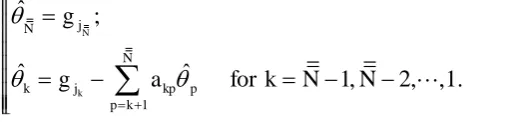
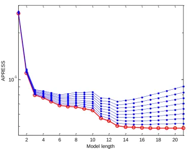
As stated in Section 2, the measurements of the transient response will be utilised in this paper to identify the dynamic model of the MR specimen. As a starting point, suppose that the term length of the elastic stiffness restoring force, the viscous damping restoring force, and the bilinear hysteresis restoring force , , in Eq.(29) are all 10. The initial model thus involves a total of 31 candidate terms. Performing the OLS algorithm indicates that the terms with the order higher than 5 and 13 for the elastic stiffness force and the viscous damping force respectively lead to ill-conditioning of the measured matrix. Therefore they should not be included into the model, that is to say, , , and . Under these assumptions, the OLS algorithm is again used to select and rank the significant model terms. By setting the adjustable parameter , the APRESS statistic versus the model length over the acquisition data, are calculated and shown in Fig. 5, where the bottom line with circles, corresponding to , indicates the mean-squared-errors. It can be seen from Fig. 5 that there is an obvious turning point at the abscissa 13 for various values of the adjustable parameter . The indexes of the first 13 model terms selected and ranked in order of the significance by the OLS algorithm, together with the coefficient of each term and its corresponding ERR, are shown in Table 1. Table 1 indicates that the terms with the cubic, quintic and linear stiffness restoring forces, the linear and quintic damping restoring forces, and the approximating Chebyshev series of maximum degree 7 should be included within the model. Representing the dynamic model using these 13 terms and performing the OLS algorithm over the measurements once again gives the estimation of the model parameters. Then after solving Eq.(37), the final identified model is obtained,
3 5 5
1 0 3 0 5 0 1 5
1 sgn
2
s
s
k y t
y
k
y t
y
k
y t
y
c y t
c y t
z t
F t
k
dz t
z
z t
dy t
(67)
where , , ,
, , , and
m, which is corresponding to the preload .
[image:13.595.182.441.76.137.2]Notice that the quintic damping term is selected at a later stage by the OLS algorithm and the ERR listed in Table 1 also indicates that it is less significant compared with other selected terms. In fact as aforementioned, the model without the quintic viscous damping force has already been used to model MR devices by some researchers although it is shown here for the first time how the model structure of MR devices can be automatically detected from the experimental data only. Since the damping of MR devices consists of a viscous damping component, the hysteretic effects are rate dependent. Actually, the experimental results have demonstrated that the hysteretic effects of MR devices depend not only the input frequency but also the input amplitude. However, a generalised dynamic model can be obtained by following the same procedure in this paper under a series of excitations with interested amplitudes and frequencies and then expressing the model coefficients as a function of the input amplitude and frequency. This is currently being studied and will be reported in a later paper.
6. Conclusions
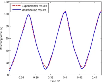
A semi-constitutive model that involves nonlinear elastic stiffness, nonlinear viscous damping and bilinear hysteretic Coulomb damping, which was later approximated by Chebyshev polynomials of the first kind, has been adopted to model MR devices. Then an efficient OLS algorithm, regularised by the APRESS criterion, was developed for model structure detection and parameter estimation. By utilising the transient response of a MR specimen, it has been shown for the first time how the model structure of MR devices can be automatically detected and then the model parameters can be estimated. The identified model agrees with the experimental results very well. It is believed that the basic ideas and algorithms developed in this paper can form an important basis for the modelling of MR devices and thus promote the theoretical analysis in this important research area.
This paper has concentrated on the model identification utilising the transient response of the MR device. Although the obtained model can provide lots of information about the properties of the MR device, MR devices often work in steady state and the model structure detection and parameter estimation utilising the steady state response will provide a more accurate and practical model, which is more meaningful for the analysis and design of metal rubber. This will be studied in a later publication.
Acknowledgement
The authors gratefully acknowledge that this work was supported by the Engineering and Physical Sciences Research Council (EPSRC), UK and the European Research Council. They are grateful to Professor Jie Hong, Beihang University (China), for providing the metal rubber specimen.
References
[1] . E. ero ɑe , "The Design of Metal Rubber Component," Z. Z. Li, translated in Chinese, National Defence Industry Press, Beijing, 2000.
[2] D. W. Childs, "Space-shuttle main engine high-pressure fuel turbopump rotodynamic instability problem," Journal of Engineering for Power-Transactions of the ASME, vol. 100, pp. 48-57, 1978. [3] A. Okayasu, et al., "Vibration problems in the LE-7 LH2 turbopump," Proceedings of the 26th AIAA
Joint Propulsion Conference, Orlando, Florida, pp. 1-5, 1990.
[4] M. Zarzour and J. Vance, "Experimental evaluation of a metal mesh bearing damper," Journal of Engineering for Gas Turbines and Power-Transactions of the ASME, vol. 122, pp. 326-329, Apr 2000. [5] E. M. Al-Khateeb, "Design, modelling, and experimental investigation of wire mesh vibration
dampers," Ph.D. Thesis, Texas A&M University, 2002.
[6] B. H. Ertas and H. G. Luo, "Nonlinear dynamic characterization of oil-free wire mesh dampers," Journal of Engineering for Gas Turbines and Power-Transactions of the ASME, vol. 130, pp. 032503-(1-8), May 2008.
[7] H. Zuo, et al., "The compression deformation mechanism of a metallic rubber," International Journal of Mechanics and Materials in Design, vol. 2, pp. 269-277, 2005.
[8] X. Wang and Z. G. Zhu, "A ringlike metal rubber damper," Journal of Aerospace Power, vol. 12, pp. 143-145, 1997.
[10] H. R. Ao, et al., "Study on the damping characteristics of MR damper in flexible supporting of turbo-pump rotor for engine," Proceedings of the 1st International Symposium on Systems and Control in Aerospace and Astronautics, Harbin, China, pp. 618-622, 2006.
[11] Y. H. Ma, et al., "Static characteristics of metal rubber," Journal of Aerospace Power, vol. 19, pp. 326-330, 2004.
[12] C. X. Yang, et al., "Research on dynamic performance of metal rubber damper," Acta Aeronautica Et Astronautica Siniga, vol. 27, pp. 536-539, 2006.
[13] Y. Y. Li and X. Q. Huang, "Influencing factors of damping characteristic for metal rubber," Journal of Vibration, Measurement & Diagnosis, vol. 29, pp. 23-26, 2009.
[14] B. T. Guo, et al., "Theoretical model of metal rubber," Journal of Aerospace Power, vol. 19, pp. 314-319, 2004.
[15] Y. Y. Li, et al., "A theoretical model and experimental investigation of a nonlinear constitutive equation for elastic porous metal rubbers," Mechanics of Composite Materials, vol. 41, pp. 303-312, Jul-Aug 2005.
[16] Y. Y. Li and X. Q. Huang, "Constitutive relation for metal rubber with different density and shape factor," Acta Aeronautica Et Astronautica Siniga, vol. 29, pp. 1084-1090, 2008.
[17] M. Brokate and J. Sprekels, "Hysteresis and Phase Transitions," Springer-Verlag, New York, 1996. [18] A. Visintin, "Differential Models of Hysteresis " Springer-Verlag, New York, 1995.
[19] J. H. Oh and D. S. Bernstein, "Semilinear Duhem model for rate-independent and rate-dependent hysteresis," IEEE Transactions on Automatic Control, vol. 50, pp. 631-645, May 2005.
[20] L. O. Chua and S. C. Bass, "A generalized hysteresis model," IEEE Transactions on Circuit Theory, vol. Ct19, pp. 36-&, 1972.
[21] M. L. Hodgdon, "Applications of a theory of ferromagnetic hysteresis," IEEE Transactions on Magnetics, vol. 24, pp. 218-221, Jan 1988.
[22] A. M. Ulanov and G. V. Lazutkin, "Description of an arbitrary multi-axial loading process for non-linear vibration isolators," Journal of Sound and Vibration, vol. 203, pp. 903-907, Jun 26 1997. [23] H. R. Ao, et al., "Dry friction damping characteristics of a metallic rubber isolator under
two-dimensional loading processes," Modelling and Simulation in Materials Science and Engineering, vol. 13, pp. 609-620, Jun 2005.
[24] W. Li, et al., "Parameter identification of nonlinear hysteretic systems based on genetic algorithm," Journal of Vibration and Shock, vol. 19, pp. 9-11, 2000.
[25] D. W. Li, et al., "Modelling of a nonlinear system with hysteresis characteristics," Chinese Journal of Mechanical Engineering, vol. 41, pp. 205-214, 2005.
[26] Q. Liu, et al., "Experimental study on a vibration isolation system with viscous damping and cubic nonlinear stiffness," Journal of Vibration and Shock, vol. 26, pp. 135-142, 2007.
[27] Y. Y. Li, et al., "Investigation on the computional method of vibration response of five power nonlinear dry friction system for metallic rubber " Journal of Astronaustics, vol. 26, pp. 620-624, 2005. [28] T. K. CAUGHEY, "Sinusoidal excitation of a system with bilinear hysteresis," Journal of Applied
Mechanics, vol. 27, pp. 640-643, 1960.
[29] W. D. Iwan and L. D. Lutes, "Response of bilinear hysteretic system to stationary random excitation," Journal of the Acoustical Society of America, vol. 43, pp. 545-552, 1968.
[30] M. J. D. Powell, "Approximation Theory and Methods " Cambridge University Press, Cambridge, 1981.
[31] H. Y. Hu and Y. F. Li, "Parametric identification of nonlinear vibration isolators with memory," Journal of Vibration Engineering, vol. 2, pp. 17-27, 1989.
[32] W. J. Cody, "A survey of practical rational and polynomial approximation of functions," Siam Review, vol. 12, pp. 400-423, 1970.
[33] S. D. Silvey, "Multicollinearity and Imprecise Estimation," Journal of the Royal Statistical Society Series B-Statistical Methodology, vol. 31, pp. 539-&, 1969.
[34] Q. Rong, et al., "Adjusted least square approach for diagnosis of ill-conditioned compliant assemblies," Journal of Manufacturing Science and Engineering, vol. 123, pp. 453-461, 2001.
[35] S. A. Billings, et al., "Identification of nonlinear output-affine systems using an orthogonal least squares algorithm," International Journal of Systems Science, vol. 19, pp. 1559-1568, Aug 1988. [36] S. A. Billings and K. M. Tsang, "Spectral analysis for nonlinear systems: 1. Parametric nonLinear
spectral analysis," Mechanical Systems and Signal Processing, vol. 3, pp. 319-339, Oct 1989.
[37] S. Chen, et al., "Orthogonal least squares methods and their application to nonlinear system identification," International Journal of Control, vol. 50, pp. 1873-1896, Nov 1989.
[39] S. A. Billings and H. L. Wei, "An adaptive orthogonal search algorithm for model subset selection and non-linear system identification," International Journal of Control, vol. 81, pp. 714-724, May 2008. [40] X. Hong and C. J. Harris, "Nonlinear model structure detection using optimum experimental design
and orthogonal least squares," IEEE Transactions on Neural Networks, vol. 12, pp. 435-439, Mar 2001. [41] X. Hong, et al., "A robust nonlinear identification algorithm using PRESS statistic and forward
regression," IEEE Transactions on Neural Networks, vol. 14, pp. 454-458, Mar 2003.
[42] X. Hong, et al., "Model selection approaches for non-linear system identification: a review," International Journal of Systems Science, vol. 39, pp. 925-946, 2008.
Table 1 The model terms selected and ranked in order of the significance by the OLS algorithm together with the coefficient of each term and its corresponding ERR.
index 2 4 3 12 1 16 18
terms k3 c1 k5 a1 k1 a5 a7
ERR 97.57% 2.0111% 0.20186% 0.017059% 0.020169% 0.018927% 0.0061967%
index 14 17 11 13 6 15
terms a3 a6 a0 a2 c5 a4
ERR 0.0019921% 0.0069366% 0.0067529% 0.0029812% 0.0074239% 0.001445%
Fig. 1 A cylindrical metal rubber (MR) specimen.
F t
( )
cf
( )
k
f
s
k
sz
y t
( )
[image:17.595.74.516.89.683.2]z
Fig. 2 A semi-constitutive mechanical model of metal rubber.
s
z
(
y
s)
y t( )( )
z t
2
3
5
6
8
0
(
y
)
s
z
( )
z t
0
1
4
7
9
10
m y t
m1y t
o
y t
m2
y t
( )
[image:17.595.120.482.309.667.2]s
z
( )
y t
( )
z t
3
5
6
2
o
s
z
m
y
sy
4
1
[image:18.595.178.421.78.269.2]
y
mFig. 4 The steady-state bilinear hysteresis loop of a metal rubber.
Fig. 5 The APRESS statistic versus the model length: the lines from bottom to the top correspond to . The bottom line with circles, corresponding to , indicates the mean-squared-errors (MSE).
2 4 6 8 10 12 14 16 18 20
10-1
Model length
A
P
R
E
S
[image:18.595.106.475.347.641.2]Fig. 6 The bilinear hysteresis loop produced by the identified model of a metal rubber specimen.
Fig. 7 A comparison of the hysteresis loop produced by the identified model of a metal rubber specimen with that plotted directly from the corresponding experimental measurements.
-12 -10 -8 -6 -4 -2 0 2 4 6 8
x 10-4 -25
-20 -15 -10 -5 0 5 10 15 20 25
Deformation displacement (m)
B
ili
n
e
a
r
h
y
s
te
re
s
is
r
e
s
to
ri
n
g
f
o
rc
e
(
N
)
-12 -10 -8 -6 -4 -2 0 2 4 6 8
x 10-4 0
20 40 60 80 100 120
Deformation displacement (m)
R
e
s
to
ri
n
g
f
o
rc
e
(
N
)
[image:19.595.115.472.429.718.2]Fig. 8 A comparison of the restoring force produced by the identified model of a metal rubber specimen with the corresponding experimental measurements.
0.34 0.36 0.38 0.4 0.42 0.44
0 20 40 60 80 100 120
Time (s)
R
e
s
to
ri
n
g
f
o
rc
e
(
N
)