ASYMPTOTIC ANALYSIS OF
DEPENDENT RISKS AND
EXTREMES IN INSURANCE AND
FINANCE
by
Jiajun Liu
Thesis submitted in accordance with the requirements of
the University of Liverpool for the degree of Doctor in Philosophy
Abstract
In this thesis, we are interested in the asymptotic analysis of extremes and risks. The heavy-tailed distribution function is used to model the extreme risks, which is widely applied in insurance and is gradually penetrating in finance as well. We also use various tools such as copula, to model dependence structures, and ex-treme value theorem, to model rare events. We focus on modelling and analysing of extreme risks as well as demonstrate how the derived results that can be used in practice.
We start from a time risk model. More concretely, consider a discrete-time annuity-immediate risk model in which the insurer is allowed to invest its wealth into a risk-free or a risky portfolio under a certain regulation. Then the insurer is said to be exposed to a stochastic economic environment that contains two kinds of risk, the insurance risk and financial risk. The former is traditional liability risk caused by insurance loss while the later is the asset risk resulting from investment. Within each period, the insurance risk is denoted by a real-valued random variable X, and the financial riskY as a positive random variable fulfils some constraints. We are interested in the ruin probability and the tail behaviour of maximum of the stochastic present values of aggregate net loss with Sarmanov or Farlie-Gumbel-Morgenstern (FGM) dependent insurance and financial risks. We derive asymptotic formulas for the finite-ruin probability with lighted-tailed or moderately heavy-tailed insurance risk for both risk-free investment and risky investment. As an extension, we improve the result for extreme risks arising from a rare event, combining simulation with asymptotics, to compute the ruin probability more efficiently.
Next, we consider a similar risk model but a special case that insurance and financial risks following the least risky FGM dependence structure with heavy-tailed distribution. We follow the study of Chen (2011) that the finite-time ruin probability in a discrete-time risk model in which insurance and financial risks form a sequence of independent and identically distributed random pairs following a common bivariate FGM distribution function with parameter −1 ≤
derived. However, the derivation there is not valid for θ = −1. In this thesis, we complete the study by extending Chen’s work to θ =−1 that the insurance risk and financial risk are negatively dependent. We refer this situation as the least risky FGM dependent insurance risk and financial risk. The new formulas for θ = 1 look very different from, but are intrinsically consistent with, the existing one for−1< θ≤1, and they offer a quantitative understanding on how significantly the asymptotic ruin probability decreases when θ switches from its normal range to its negative extremum.
Contents
Abstract i
Contents v
List of Figures vi
Acknowledgement vii
I
Introduction
viii
1 General Introduction 1
1.1 Motivations . . . 1
1.2 Structure of the Thesis . . . 4
1.2.1 Publications . . . 6
1.2.2 Conference presentations . . . 6
2 Preliminaries 7 2.1 Notations and Conventions . . . 7
2.2 Heavy-tailed and light-tailed distribution classes . . . 8
2.2.1 Heavy-tailed distribution classes and related . . . 8
2.2.2 Light-tailed Distribution Classes . . . 11
2.3 Extreme Value Theory in Insurance and Finance . . . 12
2.4 Dependence structure . . . 15
2.4.1 Copulas . . . 15
II
Ruin Probabilities in a Discrete Time Risk Model
with Dependent Risks
20
investment 21
3.1 Introduction . . . 21
3.2 Main Results . . . 25
3.2.1 A bivariate Sarmanov distribution . . . 25
3.2.2 A bivariate FGM distribution . . . 26
3.2.3 Finite-time ruin with a risk-free investment . . . 26
3.2.4 Finite-time ruin with a moderately risky investment . . . . 28
3.2.5 Finite-time ruin with a most risky investment . . . 30
3.2.6 An extension: extreme risks in insurance and finance . . . 32
3.3 Numerical Studies . . . 33
3.4 Proofs . . . 44
3.4.1 Proof of Theorem 3.2.1 . . . 45
3.4.2 Proof of Theorem 3.2.2 . . . 47
3.4.3 Proofs of Theorem 3.2.3 and Corollary 3.2.1 . . . 50
3.4.4 Proof of Theorem 3.2.4 . . . 51
3.4.5 Proof of Theorem 5.2.4 . . . 53
3.4.6 Proof of Theorem 3.2.6 . . . 53
3.4.7 Proof of Theorem 3.2.7 . . . 54
3.4.8 Proof of Theorem 3.2.8 . . . 56
3.4.9 Proof of Corollary 3.2.4 and Corollary 3.2.5 . . . 57
4 Ruin with Insurance and Financial Risks Following the Least Risky FGM Dependence Structure 58 4.1 Introduction . . . 58
4.2 Main Results . . . 60
4.3 Proofs of Theorems 4.2.1–4.2.2 . . . 63
4.3.1 General Derivations . . . 63
4.3.2 Proof of Theorem 4.2.1 . . . 64
4.3.3 Proof of Theorem 4.2.2 . . . 66
4.4 Proofs of Corollaries 4.2.1–4.2.4 . . . 70
4.4.1 Proof of Corollary 4.2.1 . . . 70
4.4.2 Proof of Corollary 4.2.2 . . . 71
4.4.3 Proof of Corollary 4.2.3 . . . 72
4.4.4 Proof of Corollary 4.2.4 . . . 73
risk model
75
5 Infinite-time Absolute Ruin in Dependent Renewal Risk Models
with Constant Force of Interest 76
5.1 Introduction . . . 76
5.2 Main results . . . 78
5.2.1 An extension: Farlie-Gumbel-Morgenstern Copula . . . 80
5.3 Proofs of main results . . . 81
5.3.1 Proof of Theorem 5.2.1 . . . 81
5.3.2 Proof of Theorem 5.2.3 . . . 85
5.3.3 Proof of Theorem 5.2.4 . . . 87
A 93
Bibliography 108
List of Figures
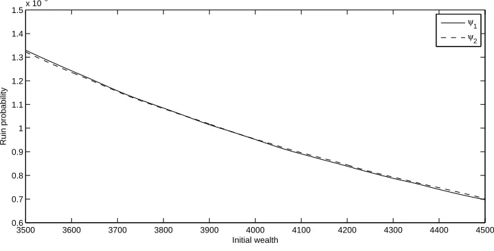
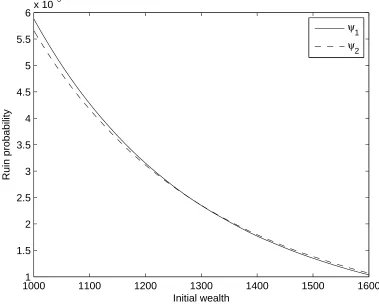
3.1 The values ofψ1(x;n) andψ2(x;n) (N = 106) . . . 36
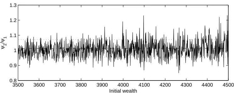
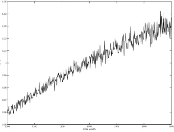
3.2 The ratio of ψ2(x;n)/ψ1(x;n) (N = 106) . . . 36
3.3 The values ofψ1(x;n) andψ2(x;n) (N = 107) . . . 37
3.4 The ratio of ψ2(x;n)/ψ1(x;n) (N = 107) . . . 38
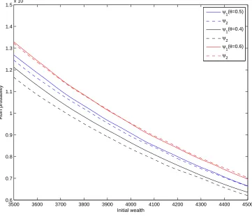
3.5 The values ofψ1(x;n) andψ2(x;n) (N = 107) . . . 39
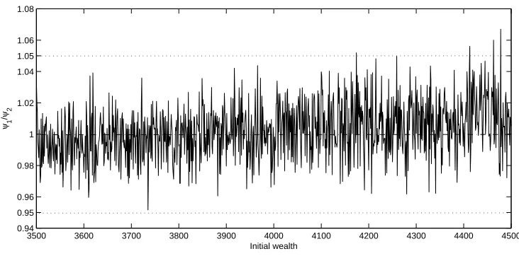
3.6 The ratio of ψ2(x;n)/ψ1(x;n) (N = 107) . . . 40
3.7 The values ofψ1(x;n) andψ2(x;n) (N = 107) . . . 40
3.8 The ratio of ψ2(x;n)/ψ1(x;n) (N = 107) . . . 41
3.9 The values ofψ1(x;n) andψ2(x;n) (N = 108) . . . 41
3.10 The ratio of ψ2(x;n)/ψ1(x;n) (N = 108) . . . 42
Acknowledgement
This thesis is the achievement of 3 years of academic research, which contains a section of research papers that I completed during my Ph.D. at the University of Liverpool. A Ph.D. can never be undertaken on your own and I am indebted to a great number of special people.
First and foremost, I would like to thank my first supervisor Dr. Yiqing Chen (Univeristy of Liverpoool & Drake University). It is she who firstly led me to research on actuarial science and guided me to find my own research interest. I really appreciate Dr Yiqing Chen’s advice and encouragement from both academic side and non-academic side in the past years. Without her help, this work would not have been possible.
Next, my thankfulness should also go to supervisor Dr. Yi Zhang (Univer-sity of Liverpool). I would like to thank him for his kind encouragement and outstanding remarks on an earlier version of this thesis in my third year. His stimulating and rigorous academic attitude has been an important effect for me to perform research at the early age.
Special acknowledgements are also given to Prof. Yang Yang (Nanjing Au-dit University). His cooperation, helpful remarks and sustained precision have increased the quality of my work.
I am grateful to Prof. Qihe Tang for the fruitful and comprehensive discussions and providing me the chance to visit the University of Iowa in 2015.
I am also very grateful to many of my colleagues and students who shared their thoughts and knowledge with me during my Ph.D. study.
Part I
Chapter 1
General Introduction
This chapter plays a role to induce the problems studied in this thesis. It will explain its motivation, background and how it contributes to the literature for each part. Furthermore, the interconnection of each part will also be expounded.
1.1
Motivations
The prevalence of rare events such as earthquake, flood, wind-storm, or terror-ism which are accompanied by disastrous economic and social consequence is the so-called Black-Swan phenomenon that make today’s world far different from decades ago. In recent years, some frequent occurrences of catastrophes include: the 2008 Sichuan Earthquake in China which costs over $148 billion, the 2008 fi-nancial crisis that directly result in the 2008-2012 global recession, the 2010 Haiti Earthquake with estimated cost between $7.2–13.2 billion, 2011 Japan Earth-quake, Tsunami and Nuclear Crisis with loss over $14.5-34.6 billion and world Banks estimated economic cost over $235 billion, the 2013 Typhoon Haiyan with damage over $1.5 billion. These catastrophes can lead to extremely large insur-ance and financial losses, which can be followed by ruin of insurinsur-ance industries or bankruptcy of financial institutions that are suffering such losses. These natural or man-made catastrophes, which make extreme losses or outliers” in statistical data, are rare events which make them particularly difficult to prognosticate; see Embrechts et al. (1997), Section 1.4 of McNeil et al. (2005), among many oth-ers. These extremes and risks have increased awareness of the need to quantify probabilities of large losses, and for helping risk management systems to control such rare events.
external event (such as flood, windstorm, forest fire, earthquake or terrorism). Therefore, they should be strongly dependent on each other. Moreover, a strong dependence among the losses can tend to make the losses jointly large. For example, properties may be damaged in a hurricane, resulting in large claims to an insurer, while they tend to be destroyed all together causes even more concern to the insurer. In extreme risk analysis, it is of particular significance to model both large individual losses and the dependence among them. To model such extreme losses and risks that are potentially large, we use light-tailed distribution and heavy-tailed distribution classes, while to model dependence, we use various tools such as copulas and joint cumulative distribution functions.
When modeling extreme losses and risks, we focus on both discrete-time and continuous-time risk models. In the first part of this thesis, we consider the ruin probabilities in a discrete time risk model with dependent risks.
The insurance business is always described by a discrete-time risk model in which the two risks that are usually called the insurance risk and the financial risk are quantified by concrete random variables. The study of the probability of ruin has become specially relevant for insurance business because of modern regulato-ry frameworks (such as EU Solvency II) that require insurance company to hold solvency capital so that the ruin probability can be taken control of. This risk model was proposed by Nyrhinen (1990, 2001). There has been a vast amount of literature in this aspect, including Norberg (1999), Tang and Tsitsiashvili (2003, 2004) and Goovaerts et al. (2005) among others. As discussed above, the insur-ance risk is referred to the risk resulting from insurinsur-ance claims and the financial risk is referred to the risk of large losses from financial investments, classifying as credit risk, market risk, operational risk, and so on. It has been commonly assumed that the insurance and financial risks are independent. However, cer-tain risks from the same policy of insurance during the successive periods or from the different policies during the same period take place in a similar environment, so that these two risks in the same time horizon should be dependent on each other. Moreover, a large number of people start to securitize their insurance risk and export it to capital market using insurance-linked securities, such as the catastrophe bounds, to hedge against catastrophic risk. Thus the insurer who invests in the capital market would like to re-insure its insurance risk, which has interconnection between the insurance risk and financial risk.
heavy-tailedness conditions. Tang and Vernic (2007) established an exact asymp-totic formula for the ruin probability, in which the financial risks constitute a stationary process with finite dimensional distributions of FGM copula. Chen and Ng (2007) obtained a formula for the ruin probability of the renewal risk model with constant interest force, in which the claims are pairwise negatively dependent and extended regularly varying tailed. Zhang et al. (2009) considered the problem of approximating the tail probability of randomly weighted sums with assumptions that claims has no bivariate upper tail dependence along with some other mild conditions. Weng et al. (2009) obtained asymptotic results for both finite and infinite ruin probabilities in a discrete time risk model with con-stant interest rates, in which the individual net losses have zero index of upper tail dependence. Recently, Chen (2011) worked out a asymptotic formula for the finite time ruin probability in a discrete time risk model with FGM dependent insurance risk and financial risks and Yang and Wang (2013) extended the result to a more general case that insurance risk and financial risk follow a bivariate Sarmanov distribution, among many others.
In the second part of this thesis, we study the ruin probabilities in a continuous-time dependent risk model. Thus far, the finite-ruin or infinite-continuous-time ruin prob-ability in a continuous-time risk model has been widely investigated by many researchers, see Asmussen (1998), Kl¨uppelberg and Stadtm¨uller (1998), Konstan-tinides et al. (2002) and Tang (2005, 2007), among many others. The standard renewal risk model was first proposed by Andersen (1957), assuming that the claim size and inter-arrival time were mutually independent, which is particular-ly paid attention to by many other researchers. In the actuarial literature, the probability of infinite-time ruin is defined to be the probability that the surplus falls below zero, which plays an unrealistic role. Compared with the research on the ordinary sense ruin probabilities, the absolute ruin probabilities have received less attention than they deserve. Moreover, the independent and identically dis-tributed (i.i.d.) assumption is for mathematical convenience but far away from reality. It is obvious that the waiting time for a claim is dependent on the claim size. Various dependence structures were introduced to the renewal risk model by many researchers. For related discussions, we refer the reader to Chen and Ng (2007), Yang and Wang (2010), Yang et al. (2013).
Monte Carlo simulations. Then computation issues arise. It is quite often that these simulations are not quite efficient when dealing with the extremely small ruin probabilities; see e.g. Tang and Yuan (2012). In addition, these simulations can not help us quantitatively understand tail behaviors of extreme losses and risks. In this thesis, we study asymptotic behaviors for extremes and risks as an alternative way to simulations. With asymptotic expressions, one can easily compute the results and it takes almost no time to get such results. Furthermore, the asymptotic expressions offer us insights that one can easily see the asymptotic behaviors of risks and how they increase comparing to some well-known quantity. For these reasons, we conduct the asymptotic tail probabilities of extreme and risks.
1.2
Structure of the Thesis
In this thesis, we study the asymptotic tail probabilities of quantities of interest in various risk models, from a discrete-time annuity-immediate risk model to a renewal risk model with constant force of interest. We investigate the impact of insurance and financial losses and how the regulations of investment affect them. We consider both light-tailed and heavy-tailed losses in our models. It turns out that the tail behavior of the loss distribution may vary in different types of insurance business.
Chapter 2 serves as a brief introduction to the theory and tools we use in this thesis.It includes notations and conventions, heavy-tailed and light-tailed distribution classes, extreme value theory, and dependence structure.
dis-counted values of aggregate net loss with Sarmanov or FGM dependent insurance and financial risks. We derive some asymptotic formulas for the finite-time ru-in probability with lighted-tailed or moderately heavy-tailed ru-insurance risk ru-in a discrete-time risk model with a risk-free or risky investment. As an extension, we improve our results to the case of extreme risks, which arise from rare events, by combining some simulation with asymptotics, to compute the ruin probabilities more efficiently.
In Chapter 4, we consider a similar discrete-time risk model but a special case that insurance and financial risks following the least risky FGM dependence struc-ture with heavy-tailed distribution. We follow the study of Chen (2011) that the finite-time ruin probability in a discrete-time risk model in which insurance and financial risks form a sequence of independent and identically distributed random pairs following a common bivariate FGM distribution function with parameter −1≤θ ≤1 governing the strength of dependence. For the subexponential case, when −1 < θ ≤ 1, a general asymptotic formula for the finite-time ruin prob-ability was derived by Chen (2011). However, the derivation there is not valid for θ = −1. In this thesis, we complete the study by extending Chen’s work to
θ = −1 that the insurance risk and financial risk are negatively dependent. We refer to this situation as the least risky FGM dependent insurance risk and fi-nancial risk. It turns out that the finite-time ruin probability behaves essentially differently for −1< θ≤1 and θ=−1.
1.2.1
Publications
Chen, Y.; Liu, J.; Liu, F. Ruin with insurance and financial risks following the least risky FGM dependence structure. Insurance: Mathematics and Economics, 62 (2015), 98–106.
Chen, Y.; Liu, J.; Yang, Y. Ruin with dependent insurance and financial risks in a discrete-time annuity-immediate risk model with a risk-free or risky investment (2015). Submitted.
Liu, J.; Yang, Y. Infinite-time absolute ruin in dependent renewal risk models with constant force of interest. Submitted.
1.2.2
Conference presentations
The workshop on New Direction in Risk Theory, Nanjing, China, November 2015, Contributed talk: “Ruin with dependent insurance and financial risks in a Discrete-time annuity-immediate risk model”.
The 19th International Congress on Insurance: Mathematics and Economics, Liverpool, UK, June 2015, Contributed talk: “Infinite-time Absolute Ruin in De-pendent Renewal Risk Model with Constant Force of Interest”.
The 18th International Congress on Insurance: Mathematics and Economics, Shanghai, China, July 2014, Contributed talk: “Ruin with Dependent Insurance and Financial Risks From light tails to Heavy tails”.
Conference in Actuarial Science and Finance on Samos, Greece, May 2014, Con-tributed talk: “Ruin with Insurance and Financial Risks Following a Special Dependence Structure”.
Chapter 2
Preliminaries
In this chapter, some mathematical concepts and tools based on which the thesis is built are provided.
2.1
Notations and Conventions
Throughout this thesis, all limit relationships are according to x → ∞ unless otherwise stated. For two positive functions f1(·) and f2(·), we write f1(x) .
f2(x) or f2(x) & f1(x) if lim supf1(x)/f2(x) ≤ 1 and write f1(x) ∼ f2(x) if limf1(x)/f2(x) = 1. We also write f1(x) f2(x) if 0 < lim inff1(x)/f2(x) ≤ lim supf1(x)/f2(x) < ∞. For convenience, we introduce a real function a(·) defined on R+ as an auxiliary function if it satisfies 0 ≤ a(x) < x/2, a(x) ↑ ∞ and a(x)/x↓0.
Furthermore, for two positive bivariate functions f1(·,·) and f2(·,·), we say the asymptotic relation f1(·,·) ∼ f2(·,·) holds uniformly for t and a non-empty set ∆ if
lim
x→∞supt∈∆
f1(x, t)
f2(x, t) −1
= 0.
Clearly, the asymptotic relationf1(·,·)∼f2(·,·) holds uniformly fort∈∆ if and only if
lim
x→∞supt∈∆
f1(x, t)
f2(x, t) ≤1 and limx→∞supt∈∆
f1(x, t)
f2(x, t) ≥1,
which mean that f1(x) . f2(x) or f1(x) & f2(x) holds uniformly for t ∈ ∆, respectively.
Let F denote the distribution function of a random variable X, whose tail is denoted by F(x) = 1−F(x) = Pr(X > x).
For two independent random variables X∗ and Y∗ with distributions F and
G, respectively, denote by F ∗G the distribution of the sum X∗ +Y∗ and by
(or sometimes as the Mellin–Stieltjes convolution) of the distributions F and G. Clearly, ifF is supported on R and G onR, then the convolution of F and G is defined as
F ∗G(x) =
Z ∞
−∞
F(x−y)G(dy) =
Z ∞
−∞
G(x−y)F(dy),
which is the distribution function of the sumX+Y. In particular, we writeF0∗
as a distribution degenerate at 0,F1∗ =F, and Fn∗ =F(n−1)∗∗F forn = 2,3, ....
Moreover, if F is supported on R and G onR+, then
F ⊗G(x) =
Z ∞
0
F
x y
G(dy), x >0. (2.1.1)
2.2
Heavy-tailed and light-tailed distribution
class-es
2.2.1
Heavy-tailed distribution classes and related
In this thesis, we follow the style of Embrechts et al. (1997) to categorize heavy-tailed distribution, although there are many criteria to define heavy-heavy-tailed dis-tribution functions in the literature. That is, a disdis-tribution function F on R is said to belong to the (right) heavy tailed distribution classK, if it holds for every
>0 that
Z ∞
0
exdF(x) = ∞.
All distribution functions not in Kare known as light-tailed distributions. In actuarial mathematics, distributions of risks or claim-size are often assumed to belong to some subclass of the heavy-tailed distribution class K. Next we in-troduce some distribution classes that will be mainly used, most being subclasses of the classK.
A distribution function F on R is said to be long tailed, written as F ∈ L, if
F(x)>0 for all x∈R+ and the relation
F(x+y)∼F(x) (2.2.1) holds for some (or, equivalently, for all) y 6= 0. For F ∈ L, automatically there is some real function l(·) with 0 < l(x) ≤ x/2 and l(x) ↑ ∞ such that relation (2.2.1) holds uniformly fory∈[x−l(x), x+l(x)]; that is,
lim
x→∞x−l(x)≤supy≤x+l(x)
F(x+y)
F(x) −1
= 0.
A distribution functionF onR+= [0,∞) is said to be subexponential, written asF ∈ S, if F(x)>0 for all x∈R+ and
F2∗(x)∼2F(x),
where F2∗ denotes the two-fold convolution of F. More generally, a distribution
function F on R is still said to be subexponential if the distribution function
F+(x) = F(x)1(x≥0) is subexponential. It is well known that S ⊂ L; see, for example, Lemma 1.3.5(a) of Embrechts et al. (1997). Subexponential distri-bution functions follow the principle of a single big jump which underlies the probabilistic behaviour of sums of independent subexponential distribution ran-dom variables. For example, for real-valued i.i.d. ranran-dom variables X1, ..., Xn
following a subexponential distribution, we have
Pr
n X
i=1
Xi > x !
∼nF(x)∼Pr
max
1≤i≤nXi > x
.
This feature explicates why subexponential distributions have become popular in modelling heavy-tailed phenomena in insurance and finance. Let F denote a distribution function andf denote its density function. We list the following well-known subexponential distributions (see Table 1.2.6 of Embrechts et al. (1997)):
• Benktander-type I: for α >0, β >0, F(x) =
1 + 2β
α lnx
exp{−β(lnx)2−(α+ 1) lnx}, x >1;
• Benktander-type II: for α >0, 0< β <1, F(x) = eα/βx−(1−β)exp
−αx
β
β
, x >1;
• Burr: forα >0, κ >0, τ >0, F(x) =
κ κ+xτ
α
, x >0;
• Loggamma: forα >0, β >0, f(x) = α
β
Γ(β)(lnx)
β−1x−α−1, x >1
• Lognormal: for−∞< µ <∞ and σ >0, f(x;µ, σ2) = √ 1
2πσxexp
−(lnx−µ) 2 2σ2
• Pareto: for α >0, κ > 0,
F =
κ κ+x
α
, x >0;
• Weibull: for a >0, 0< b <1,
F(x) = exp−axb , x > 0.
A distribution function F on Ris said to be dominatedly-varying tailed, written asF ∈ D, if F(x)>0 for all x∈R+ and the relation
F(xy) = O F(x)
holds for some (or, equivalently, for all) 0< y < 1. The intersectionL ∩ D forms a useful subclass of S; see Proposition 1.4.4(a) of Embrechts et al. (1997).
The intersection L ∩ Dcovers the class C of distributions with a consistently-varying tail. By definition, for a distribution function F onR, we write F ∈ C if
F(x)>0 for all x∈R+ and lim
y↓1 lim infx→∞
F(xy)
F(x) = 1.
Clearly, for F ∈ C it holds for every o(x) function thatF(x+o(x))∼F(x). A slightly smaller is the class R of distributions with a regularly-varying tail. By definition, for a distribution function F on R, we write F ∈ R−α for some
0≤α <∞ if F(x)>0 for all x∈R+ and the relation
F(xy)∼y−αF(x)
holds for all y >0, and we writeR the union of R−α over 0≤α <∞.
In summary, we have
R ⊂ C ⊂ L ∩ D ⊂ S ⊂ L.
Moreover, a distribution function F onRis said to be rapidly-varying tailed, written as F ∈ R−∞, if the relation
F(xy) = o F(x)
Matuszewska Indices
For a distribution F with F(x) > 0 for all x ∈ R+, its upper and lower Ma-tuszewska indices are defined as
M∗(F) = inf
−logF∗(y)
logy :y >1
and M∗(F) = sup
(
−logF
∗
(y)
logy :y >1
)
,
respectively, whereF∗(y) = lim infF(xy)/F(x) andF ∗
(y) = lim supF(xy)/F(x). It is clear that F ∈ D if and only if 0 ≤ M∗(F) < ∞, while if F ∈ R−α for
0≤α ≤ ∞then M∗(F) =M∗(F) = α.
2.2.2
Light-tailed Distribution Classes
A important subclass ofR−∞is the generalized exponential classL(γ) withγ >0,
as defined below.
A distribution F on R+ is said to be convolution-equivalent, denoted by F ∈ S(γ) for someγ ≥0 if
lim
x→∞
F(x−y)
F(x) = e
γy (2.2.2)
for every real number y and the limit lim
x→∞
F2∗(x)
F(x) = 2
Z ∞
0−
eγyF(dy) (2.2.3) exists and is finite. A larger class L(γ) is defined by relation (2.2.2) alone. If
γ = 0, the classes L(0) = L and S(0) = S are defined in Section 2.2.1. A large amount of distributions in the class S(0) such as the lognormal and the Weibull distributions also belong to the class R−∞. We remark that if γ > 0, then all
distributions in L(γ) are light-tailed.
There are some easy-verified statements which can also be found in Tang and Tsitsiashvili (2004).
(1) For a r.v. for any random variable X with its distribution belonging to the class S(γ) with γ ≥ 0, the distribution of cX with any positive constant c
belongs to the class S(γ/c);
(2) For a r.v. for two distributions F1 ∈ L(γ1) and F2 ∈ L(γ2) with some 0≤γ1 ≤γ2 <∞, we have F2(x) = o(F1(x));
(3) For a r.v. for two distribution F1 and F2 satisfying F1(x) ∼ cF2(x) for some positive constant c, then F1 is said belong to the class L(γ) or S(γ) with
γ ≥0 wheneverF2 belongs to this class;
it is known that F1 ∈ S(γ) if and only if F2 ∈ S(γ), see Kl¨uppelberg (1988). A distribution class wider than the one of all convolution-equivalent distribu-tions is the class of O-subexponential distribudistribu-tions, which was firstly introduced by Shimura and Watanabe (2005). A distribution F is said to belong the class OS, if F(x)>0 forx∈R and
F2∗(x) =O F(x)
. (2.2.4)
Kl¨uppelberg and Villasenor (1991) presented examples to show that the inclusion S(γ)⊂ L(γ)∩ OS is strict. Moreover, Lin and Wang (2012), Leslie (1989) have constructed some new distributions which belong to L(γ)∩ OS but not to S(γ) for γ >0 and for γ = 0, respectively.
2.3
Extreme Value Theory in Insurance and
Fi-nance
The prevalence of rare events such as earthquake, flood, windstorm, or terrorism which are accompanied by disastrous economic and social consequence, is so-called Black-Swan events that make today’s world far different from decades ago. Apart from the mutual exterior event, a number of highly publicised catastrophic incidents involving barings, orange county, daiwa bank, and long term capital management, have made today’s financial systems more sophisticated. These ex-tremes and risks have increased awareness of the need to quantify probabilities of large losses, and for helping risk management systems to control such rare events. There is a much longer history of using Extreme Value Theory in the insurance industry, which provides the approach to characterise the tail behaviour of the distribution without trying the analysis down to a parametric family fitted to the whole distribution. It was first derived heuristically by Fisher and Tippett (1928), which classifies distributions according to their maximum domain of attraction. The distribution functionF is said to belong to the max-domain of attraction of a univariate extreme value distribution functionF0, written F ∈MDA(F0), if
lim
n→∞supx∈
R
|Fn(anx+bn)−F0(x)|= 0 (2.3.1) holds for some suitable normalising constants an > 0, bn ∈ R, n ≥ 1. For more
details on univariate max-domains of attraction, see e.g., Reiss (1989), Embrechts et al. (1997), Falk et al. (2004), De Haan and Ferreira (2006), or Resnick (2008). A single generalised extreme value distribution was first proposed by von Miss (1936) of the form
F0ξ(x) = exp n
wherey+= max{y,0} and the right hand side is interpreted as exp{−e−x}when
ξ = 0. The regions ξ = 1/α > 0, ξ = 0 and ξ = −1/α < 0 correspond to the Fr´echet , Gumbel and Weibull cases, respectively.
The Fr´echet distribution has the cumulative distribution function Φα(x) = exp
−x−α , α, x >0
A distribution functionF belongs to MDA(Φα) if only ifF(·) is regularly varying
at infinity with index −α, that is,
lim
x→∞
F(xy)
F(x) =y
−α
holds for all y > 0; see Theorem 3.3.7 of Embrechts et al. (1997). We list the following distributions of MDA(Φα) from Table 3.4.2 of Embrechts et al.(1997).
• Burr: forα >0, κ >0, τ >0, F(x) =
κ κ+xτ
α
, x >0;
• Cauchy: forx∈R,
f(x) = π(1 +x2)−1, x∈R; • F-distribution: ford1 >0 and d2 >0,
f(x) = 1
B(d1/2, d2/2)
d1
d2
d1/2
xd21−1
1 + d1
d2
x
−d1+2d2
, x≥0;
• Loggamma: forα >0, β >0,
f(x) = α
β
Γ(β)(lnx)
β−1
x−α−1, x > 1;
• Pareto: for α >0, κ > 0,
F =
κ κ+x
α
, x >0;
• Student’s t: for v >0,
f(x) = Γ ((√ v+ 1)/2)
vπΓ(v/2)
1 + x 2
v
−(v+1)/2
The Gumbel distribution has the cumulative distribution function Λ(x) = exp−e−x , x∈
R.
A distribution function F with an upper endpoint ˆx = sup{x ∈ R : F(x) <
1} ≤ ∞belongs to MDA(Λ) if and only if the relation
lim
x↑xˆ
F(x+b(x)y)
F(x) = e
−y
holds for some positive auxiliary functionb(·) and all y ∈R, where the auxiliary function b(·) can be chosen to be the mean excess loss function:
b(x) = E(X−x|X > x).
Moreover, every distributionF from MDA(Λ) with an infinite upper endpoint also has a rapidly varying tail (see Embrechts et al. (1997), page 148). We provide some examples of MDA(Λ) from Table 3.4.2 of Embrechts et al.(1997):
• Benktander-type I: for α >0, β >0, F(x) =
1 + 2β
α lnx
exp{−β(lnx)2−(α+ 1) lnx}, x >1;
• Benktander-type II: for α >0, 0< β <1,
F(x) = eα/βx−(1−β)exp
−αx
β
β
, x >1;
• Gamma: for α >0 andβ >0, f(x) = β
α
Γ(α)x
α−1e−βx, x > 0;
• Lognormal: for−∞< µ <∞ and σ >0, f(x;µ, σ2) = √ 1
2πσxexp
−(lnx−µ) 2 2σ2
, x > 0;
• Weibull-like: for K >0, α >0, β >0, and γ ∈R
F(x)∼Kxγexp−αxβ .
The Weibull distribution is in the form of
Furthermore, a distribution function F belongs to MDA(Ψα) if only if its
endpoint ˆx is finite and the relation lim
x→∞
F(ˆx−y/x)
F(ˆx−1/x) =y
α
holds for all y > 0; see Theorem 3.3.12 of Embrechts et al. (1997). However, MDA(Ψα) can only be applied to model the bounded risk variables. The following
examples are for MDA(Ψα):
• Beta: fora >0 and b >0, f(x) = Γ(a+b)
Γ(a)Γ(b)x
a−1(1−x)b−1,0< x <1;
• Uniform: on (a, b) for 0< a < b.
2.4
Dependence structure
Recently, a new trend of research has been to introduce various dependence struc-tures to the risk model. In this direction, we refer the reader to Goovaerts et al. (2005), Tang (2006a), Zhang et al. (2009), Weng et al. (2009), Yi et al. (2011), Chen (2011) and Yang and Wang (2013), among many others.
2.4.1
Copulas
It is very important to model dependence structures in insurance and finance. The copula plays a significant role in measuring dependence. We refer the reader to Chapter 5 of McNeil et al. (2005) or the monograph Nelsen (2006) for com-prehensive applications of copulas, and see also Frees and Valdez (1998) for more details in actuarial applications.
A copula is the joint distribution function that couple the multivariate dis-tribution to standard uniform marginal disdis-tributions taking values in [0,1]. By Sklar’s theorem (Sklar (1959)), let F denote a joint distribution function with margin distribution functions F1, ..., Fn, there exists a copula C: [0,1]n → [0,1]
such that for all xi ∈R, i= 1, ..., n,
F(x1, ..., xn) = C(F1(x1), ..., Fn(xn)).
If the marginal distribution is continuous, then copula is unique; otherwise, it is unique only on Qn
i=1Ran(Fi), where Ran(Fi) denotes the range of Fi. More
There are some commonly-used copulas such as t-copulas, FGM copulas, and Archimedean copulas.
In the rest of this section, we introduce some dependence structure that mainly used in this thesis.
A Bivariate Sarmanov Distribution
Sarmanov’s family of multivariate distributions presents the advantage of having a flexible structure that is widely used to model a vast range of data dependencies. A bivarite Sarmanov distribution was firstly introduced by Sarmanov (1966) and then applied in physics by Cohen (1984) under a more general form. Lee (1996) offered a multivariate version and also discussed several applications in medicine afterwards. A more general class of bivariate distributions which includes Sar-manovs distribution was introduced by Bairamov et al. (2001). Recently, a new trend of the study is to incorporate Sarmanovs distribution in various models. Schweidel et al. (2008) used the Sarmonov family of bivariate distributions to capture the relationship between acquisition and retention. Hern´andez-Bastida et al. (2009) focused on the collective and Bayes net premiums for the aggregate amount of claims under a compound model with Sarmanov dependence between the risk profiles. Danaher and Smith (2011) demonstrated how copula models can be constructed and used in a variety of marketing applications. Hern´ andez-Bastida and Fern´andez-S´anchez (2012) developed a Sarmanov-Lee family with gamma and beta marginal distributions to apply this family in a calculating Bayes premium problem. Pelican and Vernic (2013) studied maximum-likelihood procedures for estimating Sarmanovs distribution parameters for two different models. Particularly, Vernic (2015) derived exact expressions for sums Sarmanov distributed random variables, which are useful in solving, e.g., financial and ac-tuarial problems.
Sarmanov distribution contains the popular FGM distribution. whose correla-tion coefficients cannot excess 1/3. Nevertheless, this restriccorrela-tion is not specific to the general Sarmanov distribution, see, e.g., Bairamov et al. (2001), Shubina and Lee (2004). Tang and Vernic (2006a) derive the tail asymptotics for the product of two random variablesX and Y following a bivariate FGM distribution and the distribution of X is regularly varying or rapidly-varying tailed. A more general dependence structure is studied by Yang and Wang (2013), in which they assume that (X, Y) jointly follows a bivariate Sarmanov distribution of the form
kernels, and the parameter θ is a real constant, such that
Eφ1(X) =Eφ2(Y) = 0, (2.4.2) and
1 +θφ1(x)φ2(t)≥0 for all x∈Dx, y ∈Dy, (2.4.3)
where Dx ={x ∈ R : Pr(X ∈ (x−δ, x+δ)) >0 for all δ > 0} and Dy = {y ∈
R : Pr(Y ∈ (y−δ, y+δ)) > 0 for all δ > 0}. For more details on multivariate
Sarmanov distribution, see Lee (1996) and Kotz et al. (2000). An advantage of the form (2.4.1) is that it unifies both continuous and discrete Sarmanov distri-butions. Note that if θ = 0 or φ1(x) ≡ 0, x ∈ Dx or φ2(y) ≡ 0, y ∈ Dy, then X and Y are independent. Therefore, if θ 6= 0, and the kernels φ1 and φ2 are not identical to 0 in DX and DY, we say that (X, Y) follows a proper bivariate
Sarmanov distribution. There are some common choices for kernels φ1 and φ2: (a) φ1(x) = 1−2F(x) and φ2(y) = 1−2G(y) for all x ∈ DX and y ∈ DY,
leading to the well-known Farlie-Gumbel-Morgenstern distribution (2.4.8); (b) φ1(x) = (e−x −c1)1{x≥0} with c1 = Ee−X1{X≥0}/Pr(X ≥ 0) and φ2(y) =
e−y −Ee−Y for all x ∈D
X and y∈ DY, here, 1A is the indicator function
of an event A;
(c) φ1(x) = xα and φ2(y) = yα−EYα for some α > 0 and all x ∈ DX and y∈DY.
The following lemma comes from Wang and Yang (2013), which claims that the kernels for any proper bivariate Sarmanov distribution are bounded.
Lemma 2.4.1 Assume that (X, Y) follows a proper bivariate Sarmanov distri-bution of the form (2.4.1). Then there exist two positive constantsb1 andb2 such
that |φ1(x)| ≤b1 for all x∈DX and |φ2(y)| ≤b2 for all y∈DY.
Hence, by Lemma 2.4.1, there exist two constant b1 >1 andb2 >1 such that |φ1(x)| ≤ b1 −1, |φ2(y)| ≤ b2 −1 for all x ∈ DX and y ∈ DY. It is obvious
that d1 = limx↑xˆφ1(x) < b1 with X’s upper endpoint ˆx. As in Yang and Wang (2013), introduce two independent r.v.s ˜X∗ and ˜Y∗, which are also independent of X∗,Y∗, with distributions ˜F and ˜G, respectively, defined by
˜
F(dx) =
1− φ1(x)
b1
F(dx),
and
˜
G(dy) =
1− φ2(y)
b2
here, X∗ and Y∗ are two independent r.v.s with distributions F and G, respec-tively.
Note that Lemma 2.4.1 motivates the following assumptions on the kernel functions,
lim
x↑xˆφ1(x) = d1 <∞ and limy↑yˆφ2(y) = d2 <∞, (2.4.5) with ˆxand ˆythe upper endpoints of the distributionsF andG, respectively. This implies that for anyb1 > d1 and b2 > d2,
˜
F(x)∼
1− b1
d1
F(x), x↑x,ˆ (2.4.6) and
˜
G(y)∼
1− b2
d2
G(x), y ↑y.ˆ (2.4.7)
A Bivariate Farlie-Gumbel-Morgenstern (FGM) Distribution
A brivariate Sarmanov distribution leads to the popular FGM distribution when
φ1(x) = 1−2F(x) and φ2(y) = 1−2G(y) are chosen with F onR andG onR+.
Even if there are a large number of copula families, the FGM copula is chosen since it provides the advantage of being mathematically tractable as exemplified in Cossette et al. (2009). Although the FGM copula only governs light depen-dence, it covers some positive as well as negative dependence structures between two r.v.s, and includes the independence whenθ= 0. Moreover, the FGM copula is a Taylor approximation of order one of the Frank copula, the Ali-Milkhail-Haq copula and Plackett copula, see Nelsen (2006). A brivariate FGM distribution was firstly introduced by Morgenstern (1956) and then investigated by Gumbel (1960) for exponential marginal distributions. The subsequent generalization to the current form (2.4.8) is due to Farlie (1960). For more recent discussions on FGM distributions, The reader is referred to Huang and Kotz (1999), Drouet Mari and Kotz (2001), Bairamov and Kotz (2002), Amblard and Girard (2002), and Rodr´lguez-Lallena and ´ubeda-Flores (2004), among many others. Recently, Cos-sette et al. (2008) offered an application of the generalized FGM distributions in actuarial science. Barg´es et al. (2009) carried out the problem of insurance capital allocation by assuming that the insurance risks are exponentially distributed and joined by a multivariate FGM distribution. The asymptotic behaviour of the ruin probabilityψ(x;n) in (3.1.1) was studied by Chen (2011) for the case with FGM dependent insurance and financial risks. Concretely, assume that (Xi, Yi), i∈N,
form a sequence of i.i.d. random pairs with a generic random pair (X, Y) whose components are however dependent. A bivariate FGM distribution is used to dissolve the dependence of (X, Y), which is of the form
where F on R and G on R+ are marginal distributions, and θ ∈ [−1,1] is a parameter governing the strength of the dependence, which is usually used to control the correlation coefficient of X and Y. In the study of Chen (2011), a general asymptotic result forψ(x;n) was derived for the caseθ ∈(−1,1] with the assumptions that F is subexponential, and G fulfills some constraints, in order that the product convolution ofF andGis subexponential as well. However, the derivation there is not valid for the case θ =−1. This difficulty has been solved by Chen et al. (2015), showing that the finite-time ruin probability behaves essentially differently for −1 < θ ≤ 1 and θ = −1. In this thesis, we consider some results with θ ∈ [−1,1] for the light-tailed or heavy-tailed cases under a certain regulation.
As in Chen et al. (2014), see also Yang et al. (2011), for a r.v. X, introduce two independent r.v.sX∨∗, identically distributed asX1∗∨X2∗, andX∧∗, identically distributed asX1∗∧X2∗, which are independent of all other sources of randomness, where X1∗ and X2∗ are two i.i.d. copies of X. Trivially, if X is distributed by F, then X∨∗ is distributed by F2 and the tail of X∧∗ is F
2
Part II
Ruin Probabilities in a Discrete
Time Risk Model with
Chapter 3
Ruin with Dependent Insurance
and Financial Risks in a
Discrete-time annuity-immediate
Risk Model with a Risk-free or
Risky investment
1
3.1
Introduction
An abundance of relevant research in actuarial science involves sums of depen-dent random variables. For instance, one may consider a renewal risk model with dependent claim-sizes and claim arrival times, or a discrete-time risk model with dependent insurance risks and financial risks, or the value-at-risk of a stochasti-cally discounted life annuity. Whatever kind of the risk model it is, in actuarial applications the tail distribution functions of the sums of some dependent r.v.s are particularly paid attention to. By use of asymptotic relations, the tail asymptotic behaviour of such sums can be derived in the case that the distribu-tion of the increment is light-tailed or moderately heavy-tailed. The asymptotic estimate always performs well, while some other approximations might perform worse when the heavy-tailedness increases; see e.g., Section 4.3 of Tang and Yuan (2012).
A rich amount of literature is available on the use of asymptotics in a discrete-time risk model. Nyrhinen (1999) introduced a discrete-discrete-time model and estab-lished large-deviation type estimates for the ruin probabilities. As concluded by Norberg (1999), an insurer who invests his wealth in a financial market is exposed to two kinds of risks, the insurance risk and financial risk. The former one is the traditional liability risk caused by insurance claims while the later is the asset risk
related to risky investments. Tang and Tsitsiashvili (2003, 2004) investigated the finite- and infinite-time ruin probabilities in the presence of stochastic returns on investments under the assumption that the claim-size r.v.s are i.i.d.. It is obvious that the i.i.d. assumption is far unrealistic, for example, some certain risks from the same policy of insurance during the successive periods or from the different policies during the same period take place in a similar environment. Therefore, these risks in the same time horizon should be dependent on each other, which are dominated by the same economic factors (such as regional, national or global economic growth), or impacted by a mutual exterior event (such as earthquake, flood, windstorm, forest fire, or terrorism). These rare events have increased awareness of the necessity to investigate ruin probabilities of large losses, and for risk management systems to get rid of such events. Embrechts et al. (1997) provided an exhaustive study of modelling extreme events via Extreme Value Theory (EVT) to both insurance and financial risk management. Using EVT to characterize the tail behaviour in either light-tailed or heavy-tailed case exposed to an extreme environment can make the asymptotic result more exact, see e.g. Tang et al. (2011) and Hashorva et al. (2010).
Specifically, consider a discrete-time annuity-immediate insurance risk model with insurance and financial risks in an investment portfolio as in Nyrhinen (1990) and Tang and Tsitsiashvili (2003). Within each period i, the total premium income of an insurance company is denoted by Ai and the total claim amount
plus other daily costs is denoted byBi. BothAi andBi are non-negative random
variables. We assume that the premiums are received at end of each period. Suppose that the insurer positions himself in a stochastic economic environment. To be specific, such a stochastic economic environment is referred to the financial market constituted by a risk-free investment with a constant interest rate r > 0 and a risky investment with a stochastic periodic return rate Ri ≥ −1 during
each period i, which leads to an overall stochastic accumulation factor Zi over
each period i. Usually, in the beginning of each period i, the insurer invests a proportion π ∈[0,1] of his/her current wealth in stock and keeps the remaining in the bond. Thus, with the initial wealthW0 =x, the current wealth of insurer at timen satisfies
Wn=x n Y
j=1
Zj+ n X
i=1
(Ai−Bi) n Y
j=i+1
Zj,
where the stochastic accumulation factor Zi is
Zi = ((1−π)(1 +r) +π(1 +Ri)).
Denote by a real-valued r.v. Xi = Bi − Ai, i ∈ N, the net loss (the total
discount factor (the reciprocal of the stochastic accumulation factor) is denoted by a positive r.v. Yi. In the terminology of Tang and Tsitsiashvili (2003, 2004),
{Xi, i ∈ N} and {Yi, i ∈ N} are called the insurance risks and financial risks,
respectively. In practice, under certain financial regulation,Yi takes value in the
interval (0,yˆ) with ˆy = [1 + (1−π)r]−1 in a risk-free investment strategy (i.e.
Ri ≥0) or with ˆy= (1−π)−1(1 +r)−1 involving a risky investment strategy (i.e. Ri >−1). In this framework, the probability of ruin with finite time is defined
ψ(x;n) = Pr max 1≤m≤n
m X
i=1
Xi i Y
j=1
Yj > x !
, n∈N. (3.1.1) In insurance and finance applications, there are two contrary phenomena: accumulating and discounting that we are often confronted with. The sum
Sn= n X
i=1
Xi i Y
j=1
Yj, n∈N, (3.1.2)
represents the stochastic present value of aggregate net losses up to timen, which are closely related to stochastic recurrence equations. Apart form the discrete-time risk model, there are many other examples leading sum-product stochastic structure. Theobald and Price (1984) presented the impact of nontrading effects upon the measured means, variances, and autocovariances of the returns on an index’ within a sum-product stochastic framework. Brealey and Myers (1988) of-fered an introduction on this sum-product stochastic structure within the realm of finance. Gerber (1990), Section 2.6, provided a brief introduction to perpetu-ities on stochastic recurrence equations from a life insurance point of view. Large deviations and ruin probabilities to stochastic recurrence equations with heavy-tailed innovations were investigated by Konstantinides and Mikosch (2004), in which they also claims that the stochastic recurrence equation approach has also proved useful for the estimation of GARCH and related models. Then Straumann and Mikosch (2006) studied the quasi-maximum-likelihood estimator in a general conditionally heteroscedastic time series model, in which they give conditions for existence and uniqueness of a strict stationary solution to the stochastic recur-rence equation. The random wetting transition on the Cayley tree was studied by Monthus and Garel(2009), which contains the specific structure of a Kesten variable consisting in a sum of products of random variables. Blanchet et al. (2013) focused on rare-event simulation for stochastic recurrence equations with heavy-tailed innovations.
In this thesis, we aim to investigate the maximum of the stochastic discounted values of aggregate net losses up to timen, specified as
Un = max
1≤m≤n m X
i=1
Xi i Y
j=1
The insurer has to hold enough risk reserve xto avoid risk that one can not pay its future liabilities, to be consistent with certain risk reserve regulations such as EU Solvency II, which makes the research of ruin theory particularly relevant.
Inspired by the work of Tang and Tsitsiashvili (2003), there have been a large number of papers studying the asymptotic behaviour of the ruin probability of such a discrete-time risk model in the presence of heavy-tailed insurance and fi-nancial risks. However, there is an obvious disadvantage that heavy-tailedness restriction excludes many popular distributions such as the Weibull-like, the exponential-like, the lognormal-like and the generalized inverse Gaussian distri-butions, which have been widely used to model the risk or claim size distribution in ruin theory, e.g. see Asmussen (1998). Furthermore, the distribution of the product of two light-tailed r.v.s can also belong to the class of heavy-tailed dis-tributions, e.g. see Tang (2008), Liu and Tang (2010), which is a basic element of modelling in applied areas. Since the tail behaviour of a certain complicated risk process can always be reduced to the tail behaviour of sums and products, the distribution of Un in (3.1.3) can also belong to the class of heavy-tailed
dis-tributions, although each component is light-tailed. As remarked by Embrechts et al. (1997), ruin is mainly caused by one large claim, so, corresponding to this situation, it is almost dominated by one large product of a pair of insurance and financial risks. In such circumstance, the financial riskY builds a bridge between light tails and heavy tails. Last but not least, light-tailed or moderately heavy-tailed distributions are broadly used to modelling rare events, which merit some further investigation.
In this thesis, we shall incorporate some dependence structures to this discrete-time risk model where the distribution of insurance risk X belongs to a class of light-tailed or moderately heavy-tailed distributions. At the same time, some estimators of the ultimate ruin probability are derived for the case where the insurance risk belongs to some selected class of heavy-tailed distributions. We assume that (Xi, Yi), i ∈ N, form a sequence of i.i.d. random pairs with generic
random pair (X, Y), whose components are however dependent. We firstly study a more general situation where the insurance and financial risks are dependent according to a bivariate Sarmanov distribution. Then a special case that the two risks follow a bivariate FGM distribution, will be taken into consideration. For both cases, we consider the situation that the insurer invests all his surplus into a risk-free asset, or invests partly into a risk-free asset but the remaining into a risky asset, of which the tail behaviours are essentially different in the light-tailed and moderately heavy-tailed cases. Finally, we present an extension for extreme risks through EVT to characterize the tail behaviour more exactly.
tail behaviour of the maximum of the stochastic discounted values of aggregate net loss. We are particularly interested in the issue how dependence structure affects the finite-time ruin probabilities. Section 3.2 contains the main results of this chapter, immediately following a section on an extension of extreme risks in insurance and finance. Section 3.3 performs some simulation studies to verify the approximate relationships in our main results. Finally, all of the proofs are given in Section 3.4.
3.2
Main Results
3.2.1
A bivariate Sarmanov distribution
We continue to use the notions and notation in Section 2.3. Furthermore, suppose that (Xi, Yi), i∈ N, form a sequence of i.i.d. random pairs with generic random
pair (X, Y).The components of (X, Y) are dependent and follow a joint bivariate Sarmanov distribution (2.4.1). It is easy to see that the distribution H of XY
satisfies
H(x) =
Z ∞
0
Z ∞
x/v
(1 +θφ1(u)φ2(v))F(du)G(dv)
= (1 +θb1b2) Pr(X∗Y∗ > x)−θb1b2Pr( ˜X∗Y∗ > x)
−θb1b2Pr(X∗Y˜∗ > x) +θb1b2Pr( ˜X∗Y˜∗ > x). (3.2.1) Recall Un, n ∈N, in (3.1.3). Alternatively, denote
Vn = max
1≤m≤n m X
i=1
Xi m Y
j=i
Yj, n∈N. (3.2.2)
Due to the i.i.d. assumption on the sequence {(Xi, Yi), i ∈ N}, Vn defined in
(3.2.2) is identically distributed as Un in (3.1.3), which fulfills the recursive
for-mula
V0 = 0, Vn+1 = (Vn+Xn+1)+Yn+1, n∈N.
Similarly to (3.2.1), we can write Pr(Vn+1 > x) as Pr (Vn+1 > x)
= (1 +θb1b2) Pr (Vn+X∗)+Y∗ > x
−θb1b2Pr
Vn+ ˜X∗
+
Y∗ > x
−θb1b2Pr
(Vn+X∗)+Y˜∗ > x
+θb1b2Pr
Vn+ ˜X∗
+ ˜
Y∗ > x
3.2.2
A bivariate FGM distribution
Assume that (Xi, Yi), i∈ N, form a sequence of i.i.d. random pairs with generic
random pair (X, Y).However, the components of (X, Y) are dependent and follow a joint bivariate FGM distribution of the form (2.4.8). The general derivations will be mainly used in following proofs. Since the decomposition
Π = (1 +θ)F G−θF2G−θF G2+θF2G2,
or, equivalently,
Π = (1 +θ)F G−θ(1−F2)G−θF(1−G2) +θ(1−F2)(1−G2), (3.2.4) with the fact that X∧∗ is tail distributed by F2 and Y∧∗ by G2, it follows that
H(x) = (1 +θ) Pr (X∗Y∗ > x)−θPr (X∗Y∧∗ > x)
−θPr (X∧∗Y∗ > x) +θPr (X∧∗Y∧∗ > x). (3.2.5) Applying the decomposition in (5.2.3), we have
Pr (Vn+1 > x)
= (1 +θ) Pr (Vn+X∗)+Y
∗
> x−θPr (Vn+X∧∗)+Y
∗
> x
−θPr (Vn+X∗)+Y
∗ ∧ > x
+θPr (Vn+X∧∗)+Y
∗ ∧ > x
= (1 +θ)I1−θI2−θI3+θI4. (3.2.6)
3.2.3
Finite-time ruin with a risk-free investment
We recall that the financial risksYi = ((1−π)(1 +r) +π(1 +Ri))−1, i ∈N. In
this subsection, we considered that the insurer as a risk-averse individual invests all his surplus into an almost risk-free portfolio including a fixed proportion 1−π
of a risk-free asset with a constant interest rate r and a fixed proportion π of a risk-free bond with the non-negative stochastic returns Ri ≥ 0, which indicates
that Yi takes value in the interval (0,yˆ) with ˆy = [1 + (1−π)r]−1. This implies
that ˆy∈(0,1].
In the first result, we consider a more general risk model with Sarmanov dependent insurance and financial risks.
Theorem 3.2.1 Consider a discrete-time annuity-immediate risk model with a risk-free investment. Suppose that (Xi, Yi), i ∈ N, constitute a sequence of i.i.d. random pairs with generic random pair (X, Y) following a bivariate Sarmanov distribution of the form (2.4.1) with marginal distributions F ∈ S(γ)∩ R−∞ for
someγ ≥0, and G with yˆ= [1 + (1−π)r]−1 satisfying (2.4.5). If 1 +θd
1d2 >0,
then it holds that for each n ∈N,
ψ(x;n)∼EeγVn−1Pr(X∗Y∗
whereYr∗is distributed byGrwithGr(dy) = (1+θd1φ2(y))G(dy), and independent
of X∗.
Remark 3.2.1 Note that one can extend (3.2.7) by directly applying Lemmas 3.4.4 and 3.4.3, which benefits the further numerical studies a lot, that is,ψ(x;n)∼ (1 +θd1d2)EeγVn−1Pr(X∗Y∗ > x) holds for each n∈N.
Remark 3.2.2 It seems that the above result for the Sarmanov dependence case is more general, which almost covers the FGM dependence with θ ∈ (−1,1]. However, one needs to be aware that the right hand side of the first asymptotic relation in (3.2.7) may reduce to o(Pr(X∗Y∗ > x)). Once the distribution of the insurance riskX has a rapidly-varying tail and relation (2.4.5) is satisfied, there is a possibility that the limit in (3.2.7) can sometimes correspond to a probability measure degenerate to 0 (in this case, 1 +θd1d2 = 0), see Remark 2.1 of Jiang
and Tang (2011), which is overcomed by the assumption of a proper bivariate Sarmanov distribution. Actually, observe that in the FGM case, which is a special Sarmanov case, the FGM parameter θ=−1 is excluded in Theorem 3.2.1.
In the next result, we consider the pair of dependent insurance and finan-cial risks following a bivariate FGM distribution with parameter θ in the whole interval [−1,1].
Theorem 3.2.2 In a discrete-time annuity-immediate risk model with a risk-free investment, assume that (Xi, Yi), i ∈ N, constitute a sequence of i.i.d. random pairs with generic random pair (X, Y) following a bivariate FGM distribution (2.4.8) with θ ∈ [−1,1]. If F ∈ S(γ)∩ R−∞ for some γ ≥ 0 and yˆ= [1 + (1−
π)r]−1 > 1
2, then it holds that for each n ∈N,
ψ(x;n)∼EeγVn−1Pr(X∗Y∗
θ > x)∼Ee
γVn−1Pr(XY > x), (3.2.8)
where Yθ∗, independent of X∗, is distributed by Gθ with Gθ(y) = (1−θ)G(y) + θG2(y).
Remark 3.2.3 Note that yˆ = [1 + (1 − π)r]−1 > 12 is easily satisfied since the interest rate r is always below 1 in practice. In case of a better result for numerical studies, we can rewrite (3.2.8) by applying Lemmas 3.4.5 and 3.4.6 as ψ(x;n) ∼ (1 +θ(1−pˆ))EeγVn−1Pr(X∗Y∗ > x) for θ ∈ (−1,1] and
ψ(x;n) ∼ EeγVn−1Pr(X∗Y∗
∧ > x) for θ = −1. In this section, the risk-averse
investor only invests all his wealth into a risk-free portfolio, so that there is no need to hedge the downside risks. Therefore, we reasonably assume that the in-surance risk Y has no mass at its endpoint yˆ= [1 + (1−π)r]−1 in practice, that is, pˆ= Pr(Y = ˆy) = 0, leading to ψ(x;n) ∼ (1 +θ)EeγVn−1Pr(X∗Y∗ > x) for
In the following results, we generalize the above two results to the case that the distribution of insurance risk belongs to a larger intersection classOS ∩R−∞∩
L(γ).
Theorem 3.2.3 Consider a discrete-time annuity-immediate risk model with a risk-free investment. Suppose that (Xi, Yi), i ∈ N, constitute a sequence of i.i.d.
random pairs with generic random pair (X, Y) following a bivariate Sarmanov distribution of the form (2.4.1)with marginal distributions F ∈ OS ∩ L(γ)∩ R−∞
for someγ ≥0, and Gwithyˆ= [1+(1−π)r]−1 satisfying (2.4.5). If1+θd1d2 >0,
then relation (3.2.7) holds for each n∈N.
For the special case of FGM distributions, Theorem 3.2.3 yields that
Corollary 3.2.1 In a discrete-time annuity-immediate risk model with a risk-free investment, assume that(Xi, Yi),i∈N, are a sequence of i.i.d. random pairs with generic random pair (X, Y) following a bivariate FGM distribution (2.4.8) with
θ∈(−1,1]. If F ∈ OS ∩ L(γ)∩ R−∞ for someγ ≥0, and yˆ= [1 + (1−π)r]−1,
then relation (3.2.8) holds for each n∈N.
3.2.4
Finite-time ruin with a moderately risky investment
In this subsection, we consider a more realistic case that some negative investment returns may be earned. The insurer keeps his wealth partly in a risk-free asset and invests the remaining into a risky asset, which roughly means π ∈(0,1). It is reasonable that the financial risk Y is modelled by a positive and bounded r.v. Hence, assume that the underlying financial risk in the economic environment is
¯
Y ∈ (0,∞). In the meantime, in order to hedge the downside risks, the insurer always considers to buy an option when he invests his surplus into a risky asset. Therefore, the financial risk is revised by such a strategy as
Y = ¯Y1{0<Y <¯ ˆy}+ ˆy1{yˆ≤Y <¯ ∞}
for some ˆy >1. In this strategy, the insurance riskY has a positive mass Pr(ˆy≤ ¯
Y <∞) at its endpoint ˆy. In particular, there is a economic regulation that the insurer can only partly invest his surplus into a risky asset as a matter of fact, which leads to a stochastic return rate Ri ∈[−1,∞) with Pr(Ri =−1) = ˆp≥0.
Thus, the overall return rate ˜Ri is in the form of
˜
Ri = (1−π)(1 +r) +π(1 +Ri)−1.
strategy, which has already been discussed in the previous subsection. Therefore, in order to make it possible to obtain some negative overall investment returns, the proportion π above the level r/(1 +r) is required in this subsection. Hence, if the insurer losses all the money invested into the risky asset, then the default risk is positive. Clearly, the financial risks are described asYi = ((1−π)(1 +r) + π(1 +Ri))−1, i ∈ N, which are bounded from above by ˆy = (1−π)−1(1 +r)−1
with Pr(Y = ˆy) = ˆp≥0. Consequently, the financial risk Y has a finite endpoint ˆ
y∈(1,∞) and might have a positive mass.
Now we consider a more realistic case when the insurance and financial risks are Sarmanov dependent.
Theorem 3.2.4 Consider a discrete-time annuity-immediate risk model with a moderately risky investment. Suppose that (Xi, Yi), i ∈N, constitute a sequence of i.i.d. random pairs with generic random pair (X, Y) following a bivariate Sarmanov distribution of the form (2.4.1)with marginal distributions F ∈ S(γ)∩ R−∞for someγ ≥0, andG, with a finite upper endpointyˆ= (1−π)−1(1+r)−1 >
1, satisfying (2.4.5), respectively. If 1 +θd1d2 > 0, then it holds that for each
n∈N,
ψ(x;n) ∼ Bn−1(γ) Pr X1
n Y
j=1
Yj > x !
∼ (1 +θd1d2)Bn−1(γ) Pr X∗
n Y
j=1
Yj∗ > x
!
, (3.2.9)
with
Bn−1(γ) =
n−1
Y
i=1 E
n
(1 +θd2φ1(X∗))eγˆy
−iX∗o
. (3.2.10)
Recall that the FGM copula is satisfied by the Sarmanov distribution as de-scribed in the previous subsection. However, the case θ =−1 is still excluded in Theorem 3.2.4 by a similar discussion as in Remark 3.2.2. Next we consider an extension for the FGM case with parameterθ in the whole interval [−1,1]. Theorem 3.2.5 In a discrete-time annuity-immediate risk model with a mod-erately risky investment, assume that (Xi, Yi), i ∈ N, constitute a sequence of
i.i.d. random pairs with generic random pair (X, Y) following a bivariate FGM distribution (2.4.8) with θ ∈ [−1,1]. If F ∈ S(γ)∩ R−∞ for some γ ≥0, and G
has a finite upper endpointyˆ= (1−π)−1(1 +r)−1 >1, then it holds that for each
n∈N,
ψ(x;n)∼Cn−1(γ) Pr X1
n Y
j=1
Yj > x !
with
Cn−1(γ) =
n−1
Y
i=1
(1 +θ−θpˆ) Eeγyˆ−iX∗ −θ(1−pˆ) Eeγyˆ−iX∧∗
=
n−1
Y
i=1
En(1 +θ(1−pˆ)(1−2F(X∗)))eγˆy−iX∗o. (3.2.12)
Remark 3.2.4 By Lemmas 3.4.5 and 3.4.6, we can further refine the probability on the right hand side of relation (3.2.11) as
Pr X1
n Y
j=1
Yj > x !
∼(1 +θ(1−pˆ)) Pr X∗ n Y
j=1
Yj∗ > x
!
, θ∈(−1,1],
or
Pr X1
n Y
j=1
Yj > x !
∼Pr X∗Y∧∗ n Y
j=2
Yj∗ > x
!
, θ =−1.
Next, we generalize the above two results under the condition that the distri-bution of insurance risk belongs to a larger intersection.
Theorem 3.2.6 In a discrete-time annuity-immediate risk model with a moder-ately risky investment, assume that (Xi, Yi), i∈N, constitute a sequence of i.i.d.
random pairs with generic random pair (X, Y) following a bivariate Sarmanov distribution of the form (2.4.1)with marginal distributionsF ∈ L(γ)∩OS ∩R−∞,
andG, with a finite upper endpointyˆ= (1−π)−1(1 +r)−1 >1, satisfying (2.4.5),
respectively. If 1 +θd1d2 >0, then for each n ∈N, relation (3.2.9) holds. Specially, the following result is a direct corollary of Theorem 3.2.6.
Corollary 3.2.2 In a discrete-time annuity-immediate risk model with a mod-erately risky investment, assume that (Xi, Yi), i ∈ N, are a sequence of i.i.d.
random pairs with generic random pair (X, Y) following a bivariate FGM distri-bution (2.4.8) with θ ∈(−1,1]. If F ∈ L(γ)∩ OS ∩ R−∞ for some γ ≥0, and G
has a finite upper endpoint y >ˆ 1, then relation (3.2.11) holds for each n ∈N.
3.2.5
Finite-time ruin with a most risky investment
For simplicity, we assume that there exists an auxiliary function a(·) defined onR+ such thata(x)↑ ∞, a(x)/x↓0 and
G(a(x)) =o(H∗(x)), (3.2.13)
whereH∗ is the distribution of the product of two independent r.v.s X∗ and Y∗.
Theorem 3.2.7 Consider a discrete-time annuity-immediate risk model with a most risky investment. Suppose that(Xi, Yi), i∈N, constitute a sequence of i.i.d. random pairs with generic random pair (X, Y) following a bivariate Sarmanov distribution of the form (2.4.1) with marginal distributions F ∈ L(γ)∩ R−∞
for some γ > 0, and G, with the upper endpoint yˆ = ∞, satisfying (2.4.5). If
1 +θd1d2 >0 and (3.2.13) is satisfied, then it holds that for each n ∈N,
ψ(x;n)∼Pr X1
n Y
j=1
Yj > x !
∼(1 +θd1d2) Pr X∗
n Y
j=1
Yj∗ > x
!
. (3.2.14)
Corollary 3.2.3 In a discrete-time annuity-immediate risk model with a risky investment, assume that (Xi, Yi), i ∈ N, are a sequence of i.i.d. random pairs with generic random pair (X, Y) following a bivariate FGM distribution (2.4.8) with θ ∈ (−1,1]. If F ∈ L(γ)∩ R−∞ for some γ > 0 and (3.2.13) is satisfied,
then it holds that for each n ∈N,
ψ(x;n)∼Pr X1
n Y
j=1
Yj > x !
∼(1 +θ) Pr X∗ n Y
j=1
Yj∗ > x
!
. (3.2.15) The following result compliments Corollary 3.2.3 forθ =−1, and also provides an example showing that (3.2.13) holds automatically.
Theorem 3.2.8 Consider a discrete-time annuity-immediate risk model with a risky investment. Assume that (Xi, Yi), i ∈ N, constitute a sequence of i.i.d.
random pairs with generic random pair (X, Y) following a bivariate FGM distri-bution (2.4.8) withθ=−1. IfF ∈ L(γ)∩R−∞for someγ >0andF(x)∼cG(x)
for some c >0, then it holds that for each n∈N,
ψ(x;n)∼(1 +c−1) Pr X∧∗ n Y
j=1
Yj∗ > x
!
. (3.2.16)