This is a repository copy of
Resource failures risk assessment modelling in distributed
environments
.
White Rose Research Online URL for this paper:
http://eprints.whiterose.ac.uk/79909/
Version: Accepted Version
Article:
Alsoghayer, R and Djemame, K (2014) Resource failures risk assessment modelling in
distributed environments. Journal of Systems and Software, 88. 42 - 53. ISSN 0164-1212
https://doi.org/10.1016/j.jss.2013.09.017
Reuse
Unless indicated otherwise, fulltext items are protected by copyright with all rights reserved. The copyright exception in section 29 of the Copyright, Designs and Patents Act 1988 allows the making of a single copy solely for the purpose of non-commercial research or private study within the limits of fair dealing. The publisher or other rights-holder may allow further reproduction and re-use of this version - refer to the White Rose Research Online record for this item. Where records identify the publisher as the copyright holder, users can verify any specific terms of use on the publisher’s website.
Takedown
If you consider content in White Rose Research Online to be in breach of UK law, please notify us by
Resource Failures Risk Assessment Modelling in
Distributed Environments
Raid Alsoghayera, Karim Djemameb,∗
aComputer Science Department, King Saud University, Riyadh 11543, Saudi Arabia b
School of Computing, University of Leeds, Leeds LS2 9JT, UK
Abstract
Service providers offer access to resources and services in distributed environ-ments such as Grids and Clouds through formal Service level Agreeenviron-ments (SLA), and need well-balanced infrastructures so that they can maximise the Quality of Service (QoS) they offer and minimise the number of SLA violations. We propose a mathematical model to predict the risk of failure of resources in such environments using a discrete-time analytical model driven by reliability func-tions fitted to observed data. The model relies on the resource historical data so as to predict the risk of failure for a given time interval. The model is evaluated by comparing the predicted risk of failure with the observed risk of failure, and is shown to accurately predict the resources risk of failure, allowing a service provider to selectively choose which SLA request to accept.
Keywords:
Grid Computing, Cloud Computing, Risk Assessment, Quality of Service, Resource Failure, Markov Chains
∗Corresponding author
Email addresses: [email protected](Raid Alsoghayer),[email protected]
1. Introduction
Advances in Grid/Cloud computing research have in recent years resulted in considerable commercial interest in utilising infrastructures such distributed environments provide to support commercial applications and services [1]. How-ever, significant developments in the areas of risk and dependability are neces-sary before widespread commercial adoption can become a reality. Specifically, risk management mechanisms need to be incorporated into Grid/Cloud infras-tructures, in order to move beyond the best-effort approach to service provision that current Grid infrastructures follow [2] .
Risk management is a discipline that addresses the possibility that future events may cause adverse effects and is defined in [3] as the process whereby organisations methodically address the risks attaching to their activities with the goal of achieving sustained benefit within each activity and across the portfolio of all activities.
The importance of risk management in Grid/Cloud computing is a conse-quence of the need to support various parties involved in making informed deci-sions regarding contractual agreements. Consider a provider that wishes to offer use of its resources as a pay-per-use service. Interactions between a provider and an end-user (a service consumer or a broker acting on their behalf) can then be governed through a Service Level Agreement (SLA), contractually defining the resource provider’s obligations, the price the end-user must pay and the penalty the provider needs to pay in the event that it fails to fulfil its obliga-tions. The use of SLAs to govern such interactions in Grid computing is gaining momentum [4, 5, 6]. However, such agreements represent a business risk to the parties involved. An SLA violation could be caused by various events such as a node outage or network failure. Consequently a provider may be unwilling to implement such an approach without effective risk assessment.
This paper focuses on a specific aspect of risk management as applied to Grid/Cloud computing: techniques that can be used by a resource provider to assess the risk of failure of resources within its infrastructure. This will enable a provider to identify infrastructure bottlenecks, evaluate the likelihood of an SLA violation and, where appropriate, mitigate potential risk, in some cases by identifying fault-tolerance mechanisms such as job migration to prevent SLA violations. A resource provider’s reputation is closely related to the reliability of its product (here risk assessment). The more reliable the provider’s risk assessment is, the more likely the provider is to have a favourable reputation.
A mathematical model for the prediction of the resources risk of failure is proposed with the use of a discrete-time analytical model driven by availability functions fitted to observed historical data.
This research has considered resource failures in Grid computing and the proposed mathematical model can equally be applied in a cloud environment. The main contributions of this paper are:
focuses on the statistical properties of the failure data, including the root cause of failures, the mean time between failures, and the mean time to repair.
• A model to describe the time between failures in Grid resources, as well as a model for the time to repair a resource. Modelling failures and repairs are crucial in the design of reliable systems and also when creating realistic benchmarks and test-beds for reliability testing.
• A model to predict the Grid resources risk of failure, which can also be used to rank Grid resources.
The remainder of the paper is organised as follows. Section 2 introduces the risk management discipline. Section 3 explains the vision of risk in Grid computing. Section 4 provides an overview of Grid resources failures data along with the data-collection process and presents an analysis of such data. Section 5 presents the proposed model to predict the risk of failure of a Grid resource using a discrete time analytical approach driven by reliability functions fitted to observed failures data. Section 6 presents some related work and section 7 ways to further extend this research. In conclusion, section 8 provides a summary of the research.
2. Risk Management
Risk management plays an important role in a wide range of fields, in-cluding statistics, economics, systems analysis, biology and operations re-search. The most central concepts in risk mamagement are the following: anassetis something to which a party assigns value and hence for which the party requires protection. An unwanted incident is an event that harms or reduces the value of an asset. Athreatis a potential cause of an unwanted incident whereas avulnerabilityis a weakness, flaw or deficiency that opens for, or may be exploited by, a threat to cause harm to or reduce the value of an asset. Finally, riskis the likelihood of an unwanted inci-dent and its consequence for a specific asset, andrisk levelis the level or value of a risk derived from its likelihood and consequence. For example, a server is an asset, a threat may be a computer virus, the vulnerability a virus protection not up to date, which leads to an unwanted incident: a hacker getting access to this server. The likelihood of the virus creating a back door to the server may be medium, but the integrity of the server (consequence in term sof harm) may be high.
incident: the failure of the resource. The paper only focuses on the likeli-hood(probability) of Grid resource failures, and therefore uses the terms Probability of Failure and Risk of Failure interchangeably.
3. Risk Aware Grid Computing - The Vision
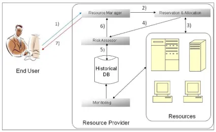
The overall vision is the production of a risk aware decision support sys-tem allowing individuals to negotiate and consume Grid resources using Service Level Agreements (SLA). This embraces an extended approach to the utility computing business model, which fits in an open market busi-ness model (for example for access to compute power) as used in sectors such as finance, automotive, and energy. This section presents the main actors (end-user and resource provider), an example scenario in which they participate, and the resource provider architectural components for risk assessment.
3.1. Actors
An end-user is a participant from a broad public approaching the Grid in order to perform a task comprising of one or more services. The user must indicate the task and associated requirements formally within an SLA template. Based on this information, the end-user wishes to negotiate access with providers offering these services, in order that the task is completed. The end-user must make informed, risk-aware decisions on the SLA quotes it receives so that the decision is acceptable and balances cost, time and risk.
A provider offers access to resources and services through formal SLAs specifying risk, price and penalty. Providers need well-balanced infrastruc-tures, so they can maximise the Quality of Service (QoS) and minimise the number of SLA violations. Such an approach increases the economic benefit and motivation of end-users to outsource their IT tasks. A prereq-uisite to this is a provider’s trustworthiness and their ability to successfully deliver an agreed SLA. The assessment of risk allows the provider to se-lectively choose which SLA requests to accept.
Figure 1: Resource Reservation and Risk Assessment - Resource Provider Components Interaction
3.2. Motivating Scenario
Considering the situation where a provider wishes to offer use of its re-sources as a pay-per-use service to potential end-users, and where the use of SLAs govern the interaction between them, a provider may need to implement an effective risk assessment prior to making an SLA offer. In this case, the provider computes the risk of failure for each resource and subsequently allocates the resources to the end-user’s job. If the resulted allocation fails to satisfy the end-user’s requirements, the resource reserva-tion is revisited; if it does satisfy the end-user’s requirements, the resource provider then sends back the SLA offer, updated with cost/penalty fee and pre-commits the resources. The end-user either commits to the SLA or rejects it.
4. Analysis of Failures in Grid Environments
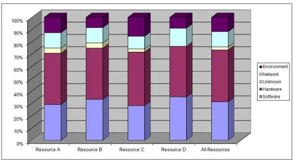
As explained in section 2 the resource provider’s assets are the Grid re-sources in the context of this paper, the Risk of Failure (ROF) of which is of great concern. Therefore, the probability of failure of a resource as well as the impact of the failure need to be identified. In order to compute such probability, the events that cause a resource to fail first need to be specified. Grid resources can fail as a result of a failure of one or more of the resource components, such as CPU or memory; this is known as hardware failure. Another event which can result in a resource failure is the failure of the operating system or programs installed on the resource; this type is known as software failure. The third event is the failure of communication with the resource; this is referred to as network failure. Finally, another event is the disturbance to the building hosting the re-source, such as a power cut or an air conditioning failure; this type is event is known asenvironmentfailure. Sometimes, it is difficult to pinpoint the exact cause of the failure, i.e. whether it is hardware, software, network, or environment failure; this is therefore referred to asunknownfailure. A setE= (EH ∪ES ∪EN ∪EE∪EU) denotes a full set of events which
include EH the events causing hardware failures, ES causing software
failures, EN causing network failures, EE causing environment failures,
andEU denoting events which cause unknown failures.
An assumption the paper makes is that the setsEH,ES,EN,EE, andEU
are disjoint (or mutually exclusive), i.e. if a resource fails at a given time
t, then only one event from the sets could have caused this failure 1. Of course, it is possible that two events or more from different sets might take place at once, yet the person responsible for the resource maintenance will only identify a single event (see section 4.1).
4.1. Failures Data Gathering
Monitored data is essential in scheduling, performance analysis, perfor-mance tuning, perforperfor-mance prediction, optimisation of Grid systems etc. Therefore, gathering data relating to past and current status of Grid re-sources is an essential activity. Monitoring resource failures is crucial in the design of reliable systems, e.g. the knowledge of failure characteristics can be used in resource management to improve resource availability [8]. Furthermore, calculating the risk of failure of a resource depends on past failures as well.
1Note that causality is the relationship between an event (the cause) and a second event
Figure 2: Breakdown of Resource Failures into Root Causes (Site 1)
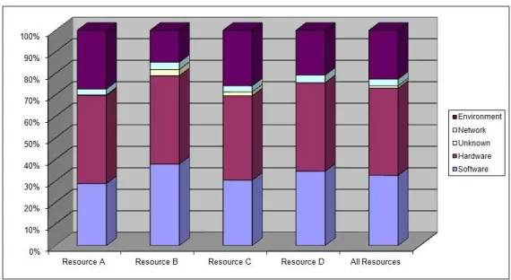
Figure 3: Breakdown of Resource Downtime into Root Causes (Site 1)
4.2. Failures Data Analysis
Resource failure data is analysed with respect to three important proper-ties of system failures: root cause breakdown, repair time, and time be-tween failures. The sequence of failure events are studied using stochastic process [14] and the distribution of its time between failures is also con-sidered. Notably, repair times are characterised for each resource using the mean, median and standard deviation. We also consider the empirical Cumulative Distribution Function (CDF) of repair time for each resource, as well as how well it fits the probability distributions commonly used in reliability theory: Exponential, Weibull, Gamma and Lognormal distribu-tions. These distributions fit the data well, and so there are no reasons for using other distributions or more degree of freedom e.g. a phase-type dis-tribution. Notably, the Maximum Likelihood Estimation (MLE) is used to parameterise the distributions and thereby evaluate the goodness of fit by visual inspection, and the negative log-likelihood test. The MLE, unlike moment estimation, is consistent, unbiased and efficient. The CDF for the time between failures for each resource is analysed also using MLE and the negative log-likelihood test [14].
Table 1: Repair Time (minutes) - Mean, Median, and Standard Deviation - Site 1
Resource A B C D
Mean 1922 1611 1658 1829
Median 945 433 1116 865
Stand.Dev. 2496 2341 2089 2346
environment failures is high, ranging between 14% and 27%. The reason for this is that the site often had air conditioning failure, which required a long maintenance work.
Therepair timemetric is investigated by considering first how the repair time varies among resources, the statistical proprieties of the repair time for each resource including their distributions, and finally how the root cause affects the repair time. Table 1 shows the mean, median and stan-dard deviation for the repair time in Site 1. The mean repair time of all resources is high because the repair time depends mainly on the availabil-ity of the Grid administrator, and this site does not have 24-hour user support. Thus, any resource failure occurring after normal working hours is not dealt with before the next working day; this also holds for week-ends and public holidays. Another reason is that there is no automatic monitoring in place that will report a resource failure when it occurs. The standard deviation shows a large spread of the data.
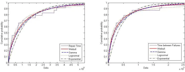
Another observation is that resource repair time is highly variable, which indicates that the Exponential distribution is not conventional to express it. With this in mind, it should be noted that an Exponential distribu-tion with failure rateλthe mean is 1/λand the median ln(2)/λ, which is 0.6931/λ[15]; thus, the mean and median should not have a huge differ-ence. To confirm this observation, the empirical Cumulative Distribution Function (CDF) for repair time in each resource is fitted with four stan-dard distributions: Exponential, Weibull, Gamma and Lognormal. The CDF - referred to as F(x) - describes the probability distribution of a real-valued random variableX to be less than x:
F(x) =P{X < x}
That is, for a given value x, F(x) is the probability that the observed value ofX will be at most x.
Figure 4: (a) Resource A Site 1 - Repair Time; (b) Time between Failures
Table 2: Resource A Site 1 - Repair Time (minutes) according to Failure Cate-gories
Category Software Hardware Network Environment Unknown
Mean 1900 1887 432 4185 1120
Median 1120 961 120 5444 1120
Stand.Dev. 2136 2710 593 3451
-resource D Weibull and Lognormal distributions create an equally good visual fit. In the following, due to space limitations the results will be shown for resource A in site 1 only.
Table 2 shows the mean, median and standard deviation for resource A site 1 repair time according to failure categories. The repair time average is 7 hours for network failures and up to 3 days for environment errors. Overall, the repair time is highly variable for all resources in site 1. An-other observation is that software and hardware failure affect individual machines, whilst a network or an environment failure, e.g. a power cut may affect a cluster or even the entire Grid site.
[image:11.612.135.475.343.395.2]The Weibull distribution is used to mathematically characterize the prob-ability of system failures as a function of time. How the time since the last failure influences the expected time until the next failure is captured by a distribution’s hazard rate function. An increasing hazard rate function predicts that the probability of failure increases with time. A decreas-ing hazard rate function predicts the reverse. The maximum likelihood estimation is used to predict the shape parameter, which is found to be 0.63 for resource A. This shape parameter of less than 1 indicates that the hazard rate function is decreasing, i.e. not seeing a failure for a long time decreases the chance of seeing one in the near future.
Random processes [17] are tested as probabilistic models for Grid resource failures [18]. The results show that random processes are not suitable for modelling Grid resources failure. The Homogeneous Poisson Process (HPP) assumes that the time between failures follows the exponential distribution, yet the time between failures in Grid environments follows a Weibull distribution. The renewal process assumes that the repair of failed component return it to as good as new state, yet in Grid environ-ments repairs do not return the resources to as good as new state. The modified renewal processassumes that the distribution of the first failure differs from the distribution of the time of the second, third or subsequent failures. This assumption is not valid in Grid environments since the dis-tribution of the time between failures follows the Weibull disdis-tribution and does not change between subsequent failures. Thealternating renewal pro-cessassumes that the distribution of the time between failures is identical and independent. In Grid environments assuming an identical distribution is inadequate. Finally the Non-Homogeneous Process (NHPP), which is widely assumed in modelling computer systems, is not fit for modelling Grid resources failure. Results in [18] show that it is highly unlikely that Grid resource failures are modelled by a NHPP following a power or ex-ponential low.
So far, the behaviour of Grid resources has been described in statistical terms. Next, a new mathematical model to assess the risk of Grid resource failures is introduced.
5. Risk of Failure Models
5.1. Availability Model
Grid resource states as shown in data collected from GOCDB (see section 4.1): up (state 0), at risk (state 1), and outage (state 2).
The memoryless property or constant failure rate assumption is a crucial assumption in Markov modelling, which is a popular technique for reliabil-ity analysis. In other words, for Grid resources the transition probabilities between states are determined by the present state only, and not by his-tory. For continuous-time models, the length of time already spent in a state does not influence either the transition rate of the next state or the remaining time in the same state before the next transition. This general assumption implies that the waiting time spent in any state is exponen-tially distributed in the continuous-time case or geometrically distributed in thediscrete-time models.
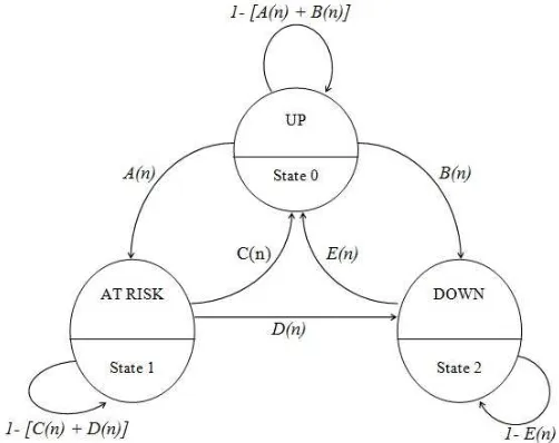
Thus, Markov models assume that failure rates are constant, thereby lead-ing to exponentially distributed inter-arrival time of failures and Poisson arrival of failures. A useful generalisation of Markov Models is the Time-Varying Markov Models, which allow state transition probability to change over time; thus, the failure rate is no longer assumed as constant [19]. With this relaxed assumption, the Grid resources can be modelled with the use of the time-varying Markov model. Since Grid resources failures and re-pairs occur at varying intervals, a continuous time-varying Markov model is used for Grid resource availability (see Figure 5). The transition matrix for the continuous time-varying Markov model is:
P(t) =
0 ZW(t) ZF(t)
ZR(t) 0 zF(t)
ZG(t) 0 0
The resource will start in State 0 (UP) and operates until either: (1) the performance degrades and the resource transits to State 1 (AT RISK); or (2) the resource stops working and transits to State 2 (DOWN). The rate of events causing transition from state 0 to 1 isZW(t) whilstZR(t) is
the rate of recovery events that result in the resource returning to State 0. Moreover, ZF(t) is the rate of events that leads to resource failure,
whereasZG(t) is the rate of repair resulting in the resource returning to
State 0.
In order to predict the Grid resource availability, the continuous time-varying Markov model is developed by applying transition functionsZW(t),
ZR(t), ZF(t), and ZG(t) derived from the distributions fitted to failure
data. Therefore, Section 5.2 deals with establishing distributions for the transition functions, whilst Section 5.3 presents the analysis of the model.
5.2. Failure Data Fitting Distributions
In order to determine the time-varying functions ZW(t), ZR(t), ZF(t),
Figure 5: Continuous Time-Varying Markov Model for Resource Avail-ability
[image:14.612.144.517.471.616.2]Figure 7: Time-Varying FunctionsZF(t) andZG(t) (Resource A Site 1)
5, the sequence of unscheduled events as well as the downtime data are analysed for each resource. There are two types of events: the first is At Risk, which represents a transition from State 0 to State 1; the second is complete failure, which represents the transition from State 0 to State 2. For each event, the time to repair the resource is recorded and represents the time to return the resource to State 0 from State 1 or 2.
The CDF of the functions ZW(t), ZR(t), ZF(t), andZG(t) for each
re-source is fitted with four standard distributions: Exponential, Weibull, Gamma and Lognormal; this helps to determine the best fit for each func-tion. The MLE is used to parameterise the distributions, and the goodness of fit is evaluated using the negative log-likelihood test.
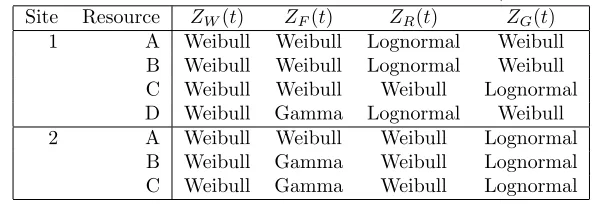
Figures 6 and 7 show that for resource A in site 1 the time between transi-tions from State 0 to 1,ZW(t), is well modelled by Weibull or Lognormal
distribution, yet the Weibull is a better fit when tested with the use of a negative log-likelihood. The time between transitions from State 0 to 2,
ZF(t), is well modelled by Weibull or Gamma; both distributions create
an equally good visual fit and the same negative log-likelihood. The repair time is the time to return the resource to State 0 from State 1 or State 2. Moreover, the time between the transitions from State 1 to State 0,
ZR(t), is well modelled by Weibull or Lognormal distribution, yet the
Log-normal is a better fit when tested with the use of a negative log-likelihood. Finally, the time between transitions from State 2 to State 0, ZG(t), is
Table 3: Best Fit Distribution for the Transition Functions (All Resources) Site Resource ZW(t) ZF(t) ZR(t) ZG(t)
1 A Weibull Weibull Lognormal Weibull
B Weibull Weibull Lognormal Weibull
C Weibull Weibull Weibull Lognormal
D Weibull Gamma Lognormal Weibull
2 A Weibull Weibull Weibull Lognormal
B Weibull Gamma Weibull Lognormal
C Weibull Gamma Weibull Lognormal
5.3. Risk of Failure Model
Following the results in Table 3 we make the assumption that the time-varying functionsZW(t),ZR(t),ZF(t), andZG(t) are based on a Weibull
probability density function with unique shape α and scale λ values for each function:
ZW(t) =αW λW(λWt)αW - 1e−(λWt)αW
ZR(t) =αR λR(λRt)αR - 1e−(λRt)αR
ZF(t) = αF λF(λFt)αF - 1e−(λFt)αF
ZG(t) =αG λG(λGt)αG - 1e−(λGt)αG
To solve the continuous time-varying Markov model the method that ap-proximates the continuous-time process with discrete-time equivalent [19] is used. Figure 8 shows the resulting discrete-time Markov model for time step δt. Since more than one transition may occur during a time step, the model must take into account the joint probability of state transition. As the state transition probabilities for the discrete-time Markov model change over time, we need to drive an expression for A(t), B(t), C(t), D(t), and E(t). This is achieved thanks to the models developed by Siewiorek and Swarz [20].
The probability transition equations are derived, in whichqij(s, t) is the
probability that the system is in statejat timetgiven that it was in state
i at time s (s ≤t). With this notation, in matrix form the Chapman-Kolmogorov equation [21] is:
Q(s, t) = Q(s, k) Q(k, t) s≤k≤t
Letting k = t - 1,
Figure 8: Discrete Time Markov Model for Resource Availability
Defining P(t) = Q(t, t + 1),
Q(s, t) = Q(s, t - 1)P(t - 1)
Expanding the equation recursively
Q(s, t) =Q(s, t−2)P(t−2)P(t−1) =Q(s, t−3)P(t−3)P(t−2)P(t−1) (1) Yielding to:
Q(s, t) =
t−1
Y
i=s
P(i) (2)
In order to translate the continuous-time probability functions into discrete-time probability functions, a discrete-discrete-time probability distribution is es-tablished that corresponds to the continuous-time distribution. The cor-responding parameters can then be calculated for the desired time-stepδt. Furthermore, a discrete-time approximation has to consider the probabil-ity of two failures during the same interval. Recall that the time-varying reliability functionsZW(t),ZR(t),ZF(t), andZG(t) are based on a Weibull
pdf = f(t) =αλ(λt)(α−1)e−(λt)α
The corresponding discrete Weibull function, probability mass function, is:
pmf = f(k) =qkα
-q(k+1)α
Given that f(k) is defined as the probability of an event occurring be-tween time ∆t and time (k + 1)∆t for some chosen interval size ∆t, the probability mass function can be expressed as:
f(k) = P[no event by k∆t] - P[no event by (k + 1)∆t] f(k) = R(k) - R(k+1)
R(k) is the reliability function. By substituting the continuous-time equiv-alents yields:
f(k) = R(k∆t) - R[(k + 1)∆t] f(k) =e−(λk∆t)α -e−(λ(k+1)∆t)α
By rearranging terms, we can find that:
q =e−(λ∆t)α
The probability mass functions ZW(t), ZR(t), ZF(t), and ZG(t) provide
the reliability for a discrete time stepn=tn/∆t. The time-varying
func-tions are:
qW =e−(λW∆t)
αW
ZW(t) = 1 -q(
t+1)αW−tαW
W
qR=e−(λR∆t)
αR
ZR(t) = 1 -q
(t+1)αR−tαR
R
qF =e−(λF∆t)
αF
ZF(t) = 1 -q
(t+1)αF−tαF
F
qG =e−(λG∆t)
αG
ZG(t) = 1 -q
(t+1)αG−tαG
G
A(t) = [1 ZF(t)]ZW(t)
B(t) = [1 ZW(t)]ZF(t)
C(t) = [1 ZF(t)]ZR(t)
D(t) = [1 ZR(t)]ZF(t)
E(t) = ZG(t)
The transition probability matrix
P(t) =
1−(A(t) +B(t)) A(t) B(t)
C(t) 1−(C(t) +D(t)) D(t)
E(t) 0 1−E(t)
– A(t) is the probability of transiting fromUptoAt Risk;
– B(t) is the probability of transiting fromUpto Down;
– C(t) is the probability of transiting fromAt RisktoUp;
– D(t) is the probability of transiting fromAt Risk toDown;
– E(t) is the probability of transiting fromDownto Up.
Taking into account thatPi,j is the probability of a transition from state
i to state j, it can then be stated that the probability of transitionP0,0is the probability of remaining in State 0, which is 1 minus the probability of leaving State 0, hence 1 - (A(t) + B(t)). The same can then be applied for the probability of transitionP1,1 andP2,2.
P(t) can be used to compute instantaneous risk of failure, which is the probability that the system will not be operational at any random time t. Another important aspect is the risk of failure duration, which refers to the probability that the system will not be operational for a certain duration (e.g. job execution time). Computing the risk of failure duration is an iterative process. Accordingly, applying the appropriate values forα
andλ, starting at S = start time,P(t) is computed forward for successive values of t until the desired finish timeT = t ∆T is reached.
5.4. Evaluation
Adopting the technique described in the previous section, the transition matrixP(t) is computed for each resource using the data from GOCDB with ∆t = 1 hour. Since Grid jobs usually require long execution times, ∆T should be selected accordingly. However, long ∆T lowers the accuracy of the model, since a state transition is not promptly recorded. On the other hand, short ∆T has the overhead of calculatingP(t) multiple times, despite the probability of transition not changing. Therefore, ∆T was selected to be 1 hour.
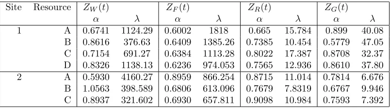
Table 4: The Shape α and Scale λ Parameters for Functions ZW(t), ZR(t),
ZF(t), andZG(t)
Site Resource ZW(t) ZF(t) ZR(t) ZG(t)
α λ α λ α λ α λ
1 A 0.6741 1124.29 0.6002 1818 0.665 15.784 0.899 40.08
B 0.8616 376.63 0.6409 1385.26 0.7385 10.454 0.5779 47.05 C 0.7154 691.27 0.6384 1113.28 0.8022 17.387 0.8708 32.37 D 0.8326 1138.13 0.6236 974.053 0.7565 12.936 0.8610 37.80
2 A 0.5930 4160.27 0.8959 866.254 0.8715 11.014 0.7814 6.676
B 1.0563 398.589 0.6806 613.096 0.7679 7.8319 0.6767 9.946 C 0.8937 321.602 0.6930 657.811 0.9098 10.984 0.7593 7.392
failures is less than 1, which means that, following a failure, the risk of another failure occuringsoonincreases. Therefore, a short time-span does not reflect the true behaviour of the resource failures.
Table 4 shows, for the resources considered, the values of the Weibull shape α and scale λ parameters for the functions ZW(t), ZR(t), ZF(t),
andZG(t). The MLE was used to estimate these parameters. The risk of
failure is calculated as the sum of the probability of transition fromUpto At Riskand the probability of transitioning fromUptoDown.
The data from GOCDB is used to validate the predicted risk of failure. Let TDown denote the time the resource is down, andTU p the time the
resource is up, the observed accumulated risk of failure is defined as:
ROF = TDown
TDown+TU p
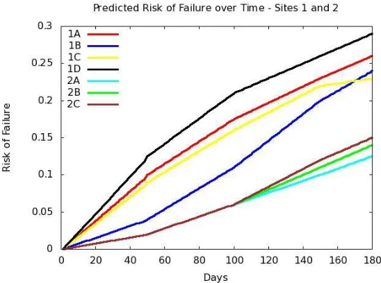
Figure 9 shows the predicted one-day duration risk of failure over a number of days, as well as the observed risk of failure for resource A (site 1). The resource observed and predicted risks of failure are clearly comparable. In order to validate the predicted risk of failure, i.e. is a true projection of the observed risk of failure, the two-samplet testis used to compare
the means of the two groups (observed and predicted risk of failure). From the above figures and the results of thet test, the conclusion is that
the risk assessment model predicts accurately the resources risk of failure. Therefore, the Grid resource provider can integrate the risk assessment model in order to compute the risk of resources failure.
Figure 9: Predicted and Observed Risk of Failure (Resource A Site 1)
[image:21.612.165.439.425.629.2]Figure 11: Resource A Site 1 Risk of Failure - with Parameters Variation (OR: Original Resource, 50DRT: 50% Decrease in Repair Time, 50ITHF: 50% Increase in Time between Hardware Failures, 50ITSF: 50% Increase between Software Failures)
In addition to ranking resources, the ROF model can be used to mea-sure the significance of the effect of changes in the Grid environment, which may include the introduction of new hardware and software, or an upgrade to the current infrastructure in order to lower resources repair time. There are various techniques for measuring this significance, the most commonly used of which is the one-at-a-time method [17]. In this case, the assumptions and parameters are changed individually so as to measure the change in output. The one-at-a-time method, along with the ROF model, are powerful tools for Grid providers to understand the limitations of current infrastructures and plan future investments. These tools are explained next.
Assume a Grid resources provider would like to make an investment to minimise the resources ROF. This investment may be on hardware and software as they are the largest contributors to failures (See section 4.2 Root Cause Breakdown), or even on experienced system administrators, expecting a decrease in the resources repair time. Therefore, an experi-ment is setup in order to investigate the effect of:
Figure 11 shows the original ROF, the ROF if the repair time is decreased by 50%, the ROF if the time between hardware failures is increased by 50% and the ROF if the time between hardware failures is increased by 50% over a number of days for Site 1, resource A. Day 0 is the time when the resource became available either after a scheduled maintenance or unscheduled failure. It can be observed that the investment in lowering the repair time is the most rewarding; this is because the repair timein the case of all resourcesis very high, even after 50% decrease. Investment in hardware or software, at this stage, is not much rewarding as the benefit on lowering the ROF is limited.
6. Related Work
The approach in this paper focuses on the risk of resource failure in Grids, which leads to three different fields of research: risk assessment/management, resource failures in distributed systems, and the use of Markov chains for problem solving. Some of the related work is reviewed next.
Risk assessment has been addressed by various projects. The objective of the Consequence project [22] is to provide an information protection framework and to thereby identify the security risk in sharing data in a distributed environment. The risk items are used as a checklist of items to be addressed in the Consequence architecture, without any assessment of the probability and the negative impact of a risk item.
The SLA@SOI project [23] does not explicitly address risk assessment, al-though it does propose the utilisation of a prediction service for estimating the probability of software and network failures, as well as hardware avail-ability in an attempt to evaluate QoS.
The AssessGrid project [2] proposes a model to estimate the probabil-ity of SLA failures in Grid environments, and considers the probabilprobabil-ity of n resources failing for the scheduled duration of a task as well as the
probability thatmreserved resources are available for that duration. The
The OPTIMIS project aims towards optimized service construction, de-ployment, and execution for Cloud Infrastructures by offering tools to efficiently manage the full life cycle of services [26]. The risk factor is considered during all phases of the service lifecycle for the two stakehold-ers: Service Providers (SP) during service construction, deployment, and operation, and Infrastructure Providers (IP) during admission control and internal operations [27].
A number of studies have looked at resource failures in distributed en-vironments [28, 8, 29, 30, 31, 32, 33, 34, 35]. Schroeder and Gibson [28] analyse failure data collected over 9 years at Los Alamos National Laboratory (LANL), and includes 23,000 failures recorded on more than 20 different systemsmostly large clusters of Symmetric-Multi-Processing (SMP) and Non-Uniform-Memory-Access (NUMA) nodes. The source of a failure falls in one of the following: human errors and environments, such as power outages, hardware failure, software failure, network failure and unknown failures. They find that the time between failure at individual nodes as well as at an entire system fit well by a Gamma or Weibull distri-bution with decreasing hazard rate (Weibull shape parameter of 0.70.8). The observation that the time between failures is best fitted by a Weibull distribution with decreasing hazard rate is also evidence in [8, 29, 30]. Io-sup et al. [35] consider the availability of CPUs in a Grid environment and analyse availability traces recorded from all the clusters. The finding is that the best fit distribution is Weibull with a shape parameter large than 1. The reason for that is that many of todays Grids comprise computing resources grouped in clusters, the owners of which may share them only for limited periods of time. Often, many of a Grids resources are removed by their owner from the systemeither individually or as complete clusters in order to serve other tasks and projects; thus, the unavailability of CPUs is not owing to a system failure but rather their unavailability by their owner. Most of the previous studies considered only short-term availabil-ity data [29]. Other studies used statistical modelling to predict failure at Grid level not resources level [30]. More importantly, these studies only consider distribution fitting to failure data.
of the next, and the unavailability subsequently becomes 2 hours. Another approach to model system availability and reliability in comput-ing is through the use of Markov models. Hacker, Romero and Carothers [31] investigated the use of Semi-Markov models to model node reliabil-ity in relation to large supercomputing systems. Platis et al. [32] adopt a two-phase cyclic non-homogeneous Markov chain with the objective to evaluate the performance of a replicated database. Koutras, Platis Grav-vanis [33] explored the use of homogeneous continuous time Markov chain with the amount of free memory to model the resource degradation of a computer system. Furthermore, the use of a cyclic non-homogeneous continuous time Markov chain in terms of driving an optimal software rejuvenation model is studied [34]. Dai, Levitin and Wang investigate maximizing the expected profit in Grid systems by partitioning the service task into subtasks and by distributing them among the available resources [36]. A genetic algorithm is presented to solve this type of optimization problem where the Grid service reliability is a critical component as the basis of the profit function. An analysis of different types of failures in Grid system and their influence on its reliability and performance is found in [37]. Models for star-topology Grid considering data dependence and tree-structure Grid considering failure correlation are presented. The uni-versal generating function, graph theory, and the Bayesian approach are used for the development of evaluation tools and algorithms. In [38] Doguc and Ramirez-Marquez discuss an automated method for estimating ser-vice reliability in Grids without relying on any assumptions about the component and link failures. The proposed method is based on a popular data mining algorithm, K2, and finds the associations between the Grid components automatically.
Other work has addressed the closely related issue of failure rates for resource components [39] such as disk failures [40]. The approach towards risk assessment is aimed at a granularity level of individual components as compared to resource level.
7. Extensions
There are many ways to further extend the work presented in this paper. The risk assessment model presented in this work only considered the re-sources historical data. An extension to this model is to consider dynamic data, such as the current resource load or the availability of administrators to enhance the model, since the mean time to repair a resource is hugely influenced by the availability of administrators.
select the best distribution for the time varying functions, e.g. Gamma, Lognormal.
Another extension to the risk model is to consider the internal components of a resource rather than considering a resource as a black-box. This extension model has different component failures, such as CPU, memory, hard drive, etc, and drives the resource risk of failure through campaigning all the component models.
The risk assessment model did not consider the type and intensity of the workload running on a resource. However, there is evidence of a correlation between the type and intensity of the workload and the failure rate of the resource [28]. More importantly, extending the model to cater for this information will provide a more accurate risk estimation.
The data used to develop the model has been provided by a research institution. The resources mean time to repair is quite due to 1) the lack of 24-hour support service, and 2) the absence of an automatic monitoring service which to report resource failures when they occur. It would be ideal to use data from commercial Grid providers, if available, to further validate the risk assessment model.
The risk assessment model was developed and evaluated analytically. There-fore, it would be beneficial to implement the model on a production Grid in order to evaluate its overall performance.
This research has considered resource failures in Grid computing and can equally be applied in cloud computing. The proposed risk assessment model, its implementation, testing, and evaluation in a cloud environment are considered in the OPTIMIS project [27, 26].
8. Conclusions
This paper has presented the steps towards the development of a mathe-matical model to predict Grid resources risk of failure.
The motivation scenario for the Grid resources risk of failure model is first presented. The events causing resource failures are identified, and the method for measuring the risk of these events is presented. The need for historical failure data is showcased, along with the data collection process.
The probability of resource failures plays a central role in the risk assess-ment process. The reviewed models found in the literature to compute this probability have clear limitations: the unrealistic assumption that the resource failures represent a Poisson process, the subjective prior distri-bution selection in the Bayesian model or ignoring resource unavailability due to scheduled maintenance. Therefore, this paper has shown that the resource failures do not represent a Poisson process, fit distributions to observed resource failures data, and use a Markov model to represent all the resource states. A continuous time-varying Markov Model described the Grid resource availability. In order to solve the Markov model, there is the need to approximate the continuous-time process with discrete-time equivalents. The resulting discrete time-varying Markov Model is used to estimate the resources risk of failure.
Such model can be integrated in the resource provider risk assessment and is a viable contender to enable the provider to identify infrastructure bottlenecks and mitigate potential risk, in some cases by identifying fault-tolerance mechanisms to prevent SLA violations.
This research can be extended in many ways: 1) consideration of dynamic data, such as the current resource load or the availability of administra-tors to enhance the model; 2) risk assessment at the level of the resource’s components (CPU, memory, hard drive, network interface card etc); 3) consideration of the type and intensity of the workload running on a re-source; 4) consideration of data from commercial Grid/Cloud providers, and 5) the implementation of the risk model on a production Grid/Cloud in order to evaluate its performance.
References
[1] F. Berman, G. Cox, A. Hey (Eds.), Grid Computing: Making the Global Infrastructure a Reality, Wiley, 2003.
[2] K. Djemame, I. Gourlay, J. Padgett, G. Birkenheuer, M. Hovestadt, O. Kao, K. Vo, Introducing Risk Management into the Grid, in: Pro-ceedings of the 2nd IEEE International Conference on e-Science and Grid Computing (eScience2006), IEEE Computer Society, Amster-dam, Netherlands, 2006.
[3] The risk management standard, Institute of Risk Man-agement. The Association of Insurance and Risk Man-agers,National Forum for Risk Management in the Public Sector, http://www.theirm.org/publications/PUstandard.html (2009).
[5] D. Battr´e, O. Kao, K. Vo, Implementing ws-agreement in a globus toolkit 4.0 environment, in: Usage of Service Level Agreements in Grids Workshop in conjunction with The 8th IEEE International Conference on Grid Computing (GRID2007), Austin, Texas, 2007.
[6] O. Waeldrich, W. Ziegler, WS-Agreement Framework for Java (WSAG4J), http://packcs-e0.scai.fraunhofer.de/mss-project/index.html (2010).
[7] K. Djemame, J. Padgett, I. Gourlay, D. Armstrong, Brokering of risk-aware service level agreements in grids, Concurrency and Com-putation: Practice and Experience 23 (7).
[8] T. Heath, R. P. Martin, T. D. Nguyen, Improving cluster availability using workstation validation, in: Proceedings of the 2002 ACM SIG-METRICS international conference on Measurement and modeling of computer systems, SIGMETRICS ’02, ACM, New York, NY, USA, 2002, pp. 217–227.
[9] Grid operations centre database, https://goc.egi.eu (2010).
[10] European grid infrastructure - towards a sustainable grid infrastruc-ture, http://www.egi.eu (2010).
[11] National grid service - connecting infrastructure, connecting research, http://www.ngs.ac.uk (2010).
[12] Worldwide lhc computing grid, http://lcg.web.cern.ch/LCG/ (2010).
[13] Cern - the european organization for nuclear research, http://www.cern.ch (2010).
[14] M. Rausand, A. Høyland, System Reliability Theory: Models, Sta-tistical Methods, and Applications, 2nd Edition, Wiley, 2008.
[15] R. Blischke, D. Murthy, Reliability: Modeling, Prediction, and Opti-mization, Wiley Series in Probability and Statistics, John Wiley and Sons, 2000.
[16] D. Murthy, M. Xie, R. Jiang, Weibull Models, Wiley-Interscience, John Wiley and Sons, 2004.
[17] M. Modarres, Risk Analysis In Engineering: Techniques, Tools, and Trends, Taylor & Francis, Boca Raton, 2006.
[19] J. Pukite, P. Pukite, Modeling for Reliability Analysis: Markov Mod-eling for Reliability, Maintainability, Safety, and Supportability Anal-yses of Complex Systems, Wiley-IEEE Press, 1998.
[20] D. Siewiorek, R. Swarz, Reliable Computer Systems: Design and Evaluation, Digital Press, 1998, 3rd edition.
[21] A. Papoulis, S. U. Pillai, Probability, random variables, and stochas-tic processes, 4th Edition, McGraw Hill, 2002.
[22] Consequence: the context-aware data-centric information sharing, http://www.consequence-project.eu (2011).
[23] Sla@soi: Slas empowering a dependable service economy, http://sla-at-soi.eu (2011).
[24] C. Carlsson, Risk Assessment for Grid Computing with Predictive Probabilities and Possibilistic Models, in: Proceedings of the 5th In-ternational Workshop on Preferences and Decisions, Trento, Italy, 2009.
[25] D. Battr´e, G. Birkenheuer, M. Hovestadt, O. Kao, K. Voss, Apply-ing Risk Management to Support SLA ProvisionApply-ing, in: The 8th Cracow Grid Workshop, Academic Computer Center CYFRONET AGH, 2008.
[26] A. J. Ferrer, F. Hernandez, J. Tordsson, E. Elmroth, A. Ali-Eldin, C. Zsigri, R. Sirvent, J. Guitart, R. M. Badia, K. Djemame, W. Ziegler, T. Dimitrakos, S. K. Nair, G. Kousiouris, K. Konstanteli, T. Varvarigou, B. Hudzia, A. Kipp, S. Wesner, M. Corrales, N. Forgo, T. Sharif, C. Sheridan, Optimis: A holistic approach to cloud service provisioning, Future Generation Computer Systems 28 (1) (2012) 66 – 77.
[27] K. Djemame, D. Armstrong, M. Kiran, M. Jiang, A risk assessment framework and software toolkit for cloud service ecosystems, in: Pro-ceedings of the Second International Conference on Cloud Comput-ing, GRIDs, and Virtualization, Rome, Italy, 2011.
[28] B. Schroeder, G. A. Gibson, A large-scale study of failures in high-performance computing systems, in: Proceedings of the International Conference on Dependable Systems and Networks, DSN ’06, IEEE Computer Society, Washington, DC, USA, 2006, pp. 249–258.
[30] F. Nadeem, R. Prodan, T. Fahringer, Characterizing, modeling and predicting dynamic resource availability in a large scale multi-purpose grid, in: Proceedings of the 2008 Eighth IEEE International Sym-posium on Cluster Computing and the Grid, CCGRID ’08, IEEE Computer Society, Washington, DC, USA, 2008, pp. 348–357.
[31] T. J. Hacker, F. Romero, C. D. Carothers, An analysis of clustered failures on large supercomputing systems, Journal of Parallel and Distributed Computing 69 (7) (2009) 652–665.
[32] A. Platis, G. Gravvanis, K. Giannoutakis, E. Lipitakis, A two-phase cyclic nonhomogeneous markov chain performability evaluation by explicit approximate inverses applied to a replicated database system, Journal of Mathematical Modelling and Algorithms 2 (2003) 235–249.
[33] V. P. Koutras, A. N. Platis, G. A. Gravvanis, Software rejuvenation for resource optimization based on explicit approximate inverse pre-conditioning, Applied Mathematics and Computation 189 (1) (2007) 163 – 177.
[34] V. P. Koutras, A. N. Platis, G. A. Gravvanis, On the optimization of free resources using non-homogeneous markov chain software reju-venation model, Reliability Engineering amp; System Safety 92 (12) (2007) 1724 – 1732.
[35] A. Iosup, M. Jan, O. Sonmez, D. Epema, On the dynamic resource availability in grids, in: Grid Computing, 2007 8th IEEE/ACM In-ternational Conference on, 2007, pp. 26 –33.
[36] Y.-S. Dai, G. Levitin, X. Wang, Optimal task partition and distri-bution in grid service system with common cause failures, Future Generation Computer Systems 23 (2) (2007) 209 – 218.
[37] Y. Dai, G. Levitin, Performability Modeling and Analysis of Grid Computing, Handbook of Performability Engineering, K.B. Misra (Ed.), Springer-Verlag, 2008, Ch. 65.
[38] O. Doguc, J. E. Ramirez-Marquez, An automated method for esti-mating reliability of grid systems using bayesian networks, Reliability Engineering System Safety 104 (0) (2012) 96 – 105.
[39] A. Sangrasi, K. Djemame, Component level risk assessment in grids: A probablistic risk model and experimentation, in: Digital Ecosys-tems and Technologies Conference (DEST), 2011 Proceedings of the 5th IEEE International Conference on, 2011, pp. 68 –75.