Reconstruction of one-dimensional chaotic maps from sequences of probability density functions

DOI 10.1007/s11071-015-1949-9 O R I G I NA L PA P E R

Reconstruction of one-dimensional chaotic maps

from sequences of probability density functions

Xiaokai Nie · Daniel Coca

Received: 29 August 2014 / Accepted: 30 January 2015 / Published online: 20 February 2015 © The Author(s) 2015. This article is published with open access at Springerlink.com

Abstract In many practical situations, it is impos-sible to measure the individual trajectories generated by an unknown chaotic system, but we can observe the evolution of probability density functions gener-ated by such a system. The paper proposes for the first time a matrix-based approach to solve the gen-eralized inverse Frobenius–Perron problem, that is, to reconstruct an unknown one-dimensional chaotic trans-formation, based on a temporal sequence of proba-bility density functions generated by the transforma-tion. Numerical examples are used to demonstrate the applicability of the proposed approach and evaluate its robustness with respect to constantly applied stochastic perturbations.

Keywords Chaotic maps·Inverse Frobenius–Perron problem·Nonlinear systems·Probability density functions

1 Introduction

One-dimensional chaotic maps describe many dynam-ical processes, encountered in engineering, biology,

X. Nie·D. Coca (

B

Department of Automatic Control and Systems Engineering, The University of Sheffield, Sheffield S1 3JD, UK

e-mail: d.coca@sheffield.ac.uk X. Nie

e-mail: x.nie@sheffield.ac.uk

physics and economics [1], which generate density of states. Examples include particle formation in emulsion polymerization [2], papermaking systems [3], bursty packet traffic in computer networks [4,5], cellular uplink load in WCDMA systems [6]. A major chal-lenge is that of inferring the chaotic map that describes the evolution of the unknown chaotic system, solely based on experimental observations.

Starting with seminal papers of Farmer and Sidorovich [7], Casadgli [8] and Abarbanel et al. [9], the problem of inferring dynamical models of chaotic systems directly from time series data has been addressed by many authors using neural networks [10], polynomial [11] or wavelet models [12].

In many practical applications, it is more convenient to observe experimentally the evolution of the prob-ability density functions, instead of individual point trajectories, generated by such systems. For example, the particle image velocimetry (PIV) method of flow visualization [13] allows identifying individual tracer particles in each image, but not to track these between images. In biology, flow cytometry is routinely used to measure the expression of membrane proteins of indi-vidual cells in a population [14]. However, it is impos-sible to track the cells between subsequent analyses.

problem for a very restrictive class of piecewise con-stant density functions, using graph-theoretical meth-ods. Ershov and Malinetskii [16] proposed a numeri-cal algorithm for constructing a one-dimensional uni-modal transformation which has a given invariant den-sity. The results were generalized in Góra and Boyarsky [17], who introduced a matrix method for constructing a 3-band transformation such that an arbitrary given piecewise constant density is invariant under the trans-formation. Diakonos and Schmelcher [18] considered the inverse problem for a class of symmetric maps that have invariant symmetric Beta density functions. For the given symmetry constraints, they show that this problem has a unique solution. A generalization of this approach, which deals with a broader class of continu-ous unimodal maps for which each branch of the map covers the complete interval and considers asymmet-ric beta density functions, is proposed in [19]. Huang presented approaches to constructing smooth chaotic transformation with closed form [20,21] and multi-branches complete chaotic map [22] given invariant densities. Boyarsky and Góra [23] studied the problem of representing the dynamics of chaotic maps, which is irreversible by a reversible deterministic process. Baranovsky and Daems [24] considered the problem of synthesizing one-dimensional piecewise linear Markov maps with prescribed autocorrelation function. The desired invariant density is then obtained by perform-ing a suitable coordinate transformation. An alterna-tive stochastic optimization approach is proposed in [25] to synthesize smooth unimodal maps with given invariant density and autocorrelation function. An ana-lytical approach to solving the IFPP for two specific types of one-dimensional symmetric maps, given an analytic form of the invariant density, was introduced in [26]. A method for constructing chaotic maps with trary piecewise constant invariant densities and arbi-trary mixing properties using positive matrix theory was proposed in [5]. The approach has been exploited to synthesize dynamical systems with desired charac-teristics, i.e. Lyapunov exponent and mixing properties that share the same invariant density [27] and to analyse and design the communication networks based on TCP-like congestion control mechanisms [28]. An extension of this work to randomly switched chaotic maps is stud-ied in [29]. It is also shown how the method can be extended to higher dimensions and how the approach can be used to encode images. In [30], the inverse prob-lem is formulated as the probprob-lem of stabilizing a target

distribution using an open-loop perturbation approach. In order to characterize the patterns of activity in the olfactory bulb, an optimization approach was proposed to infer the elements of the Frobenius–Perron matrices that encode the invariant density functions of interspike intervals corresponding to different odours [31].

All existing methods can be used to construct a map with a given invariant density. A limitation of these approaches is that the solution to the inverse problem is not unique. Typically, there are many transforma-tions, exhibiting a wide variety of dynamical behav-iours, which share the same invariant density. There-fore, the reconstructed map does not necessarily exhibit the same dynamics as the underlying systems even though it preserves the required invariant density. Addi-tional constraints and model validity tests have to be used to ensure that the reconstructed map captures the dynamical properties of the underlying system (Lya-punov exponents, fixed points, etc.) and predicts its evolution. This is of paramount importance in a many practical applications ranging from modelling and con-trol of particulate processes [48], characterizing the formation and evolution of the persistent spatial struc-tures in chaotic fluid mixing [32], characterizing the chaotic behaviour of electrical circuits [33], chaotic sig-nal processing [34,35], asig-nalysing and interpreting cel-lular heterogeneity [36,37] and identification of mole-cular conformations [38]. Potthast and Roland [39] solved the Frobenius–Perron equation describing the evolution of uniform probability distributions under the action of nonlinear dynamical automata that imple-ment Turing machines. In this context, the realization of nonlinear dynamical automata that describe cognitive processes based on experimental data can be formu-lated as an inverse Frobenius–Perron problem.

Another major limitation of the existing matrix-based reconstruction algorithms is the assumption that the Markov partition is known in advance. In general, no a priori information about the unknown map is avail-able, so the partition identification problem has to be solved as part of the reconstruction method.

esti-mation of the Frobenius–Perron matrix and the recon-struction of the underlying map.

To our knowledge, our approach provides for the first time a solution to the problem of inferring, from sequences of density functions, a broad class of one-dimensional transformations that admit an invariant density when the Markov partition is not known in advance.

This paper is organized as follows: in Sect,2, we give a brief introduction to the inverse Frobenius– Perron problem. The methodology for reconstructing piecewise-linear semi-Markov transformations from sequences of densities is presented and demonstrated using a numerical simulation example in Sect.3. An extension of the method to continuous nonlinear trans-formations is introduced and demonstrated numerically in Sect.4. Conclusions are presented in Sect.5.

2 The inverse Frobenius–Perron problem

Let I = [a,b],B be a Borel σ-algebra of subsets in I , andμdenote the normalized Lebesgue measure on I . Let S : I → I be a measurable, non-singular

transformation, that is,μ(S−1(A))∈Bfor any A∈B andμ(S−1(A))=0 for all A∈Bwithμ(A)=0. If xn

is a random variable on I having the probability density function fn ∈ D(I,B, μ),D = {f ∈ L1(I,B, μ) :

f ≥0,f1=1}, such that

Prob{xn∈ A} =

A

fndμ, (1)

then xn₊1given by

xn+1=S(xn), (2)

is distributed according to the probability density func-tion fn+1 = PSfn, where PS : L1(I) → L1(I),

defined by

A

PSfndμ=

S−1_(A)

fndμ, (3)

is the Frobenius–Perron operator [40] associated with the transformation S. In this case, PS can be written

explicitly as

fn+1(x)=PSfn(x)=

d dx

S−1_([a,s])

fn(s)ds, (4)

The Frobenius–Perron operator of a non-singular trans-formation S is a Markov operator [41].

Definition 1 A linear operator PS:L1→L1

satisfy-ing

(a) PSfn≥0 for fn≥0, fn∈L1;

(b) PSL1 <1, andPSfnL1 = fnL1, for fn≥0,

fn∈ L1,

is called a Markov operator.

Definition 2 A Markov operator PS : L1 → L1

is called strongly constrictive if there exists a com-pact set F ⊂ L1 such that for any fn ∈ D,

limn→∞dist(Pnf,F) = 0, where dist(Pnf,F) =

inff∈Ff −PnfL1.

If PSis strongly constrictive, according to the

spec-tral decomposition theorem [40], there exist a sequence of densities f1, . . . , fr and a sequence of bounded

lin-ear functionals g1, . . . ,gr such that

lim

n→∞

PSn

f −

r

i=1 gi(f)fi

L1

=0,

for any f ∈ L1. (5)

where P_Sn is the nth iteration of P, the densities

f1, . . . , fr have mutually disjoint supports ( fifj =

0 for i = j), and PSfi = fα(i), i = 1, . . . ,r

and{α(1), . . . , α(r)}is a permutation of the integers

{1, . . . ,r}. Furthermore, P_Snf converges to an invariant

density f∗, which satisfies f∗=PSf∗.

LetR= {R1,R2, . . . ,RN}be a partition of I into

intervals, and int(Ri)∩int(Rj)=∅if i = j . If S is a

piecewise monotonic transformation

PSfn(x)= N

i=1 fn

S_i−1(x) S

S_i−1(x) −1χS(Ri)(x),

(6)

where Siis the monotonic segment of S on each interval

Ri.

The inverse Frobenius–Perron problem is usually formulated [17] as the problem of determining the point transformation S such that the dynamical system

xn+1=S(xn)has a given invariant probability density

function f∗. In general, the problem does not have a unique solution.

{xj

0,i}θ, K

i,j=1 and {x

j

1,i}θ, K

i,j=1 be two sets of initial and final states observed in K separate experiments, where

x₁j_,i = S(x₀j_,i), i = 1, . . . , θ, j = 1, . . . ,K , and S :I → I is an unknown, non-singular point

transfor-mation. We assume that for practical reasons, we can-not associate with an initial state x₀j_,ithe corresponding image x₁j_,i, but we can estimate the probability density functions f₀jand f₁jassociated with the initial and final states,{x₀j_,i}θ_i=1and{x₁j_,i}θ_i=1, respectively. Moreover, let f∗be the observed invariant density of the system. The inverse problem is to determine S : I → I such

that f₁j = PSf₀jfor j =1,K and f∗=PSf∗.

3 A solution to the IFPP for piecewise-linear semi-Markov transformations

This section presents a method for solving the IFPP for a class of piecewise monotonic and expanding trans-formations calledR-semi-Markov [17], where

R= {R1,R2, . . . ,RN}

= {[c0,c1], (c1,c2], . . . , (cN−1,cN]}, (7)

is a partition of I = [a,b], c0=a, cN =b.

Definition 3 A transformation S : I → I is said to

be semi-Markov with respect to the partitionR(orR -semi-Markov) if there exist disjoint intervals Q(_ji) so that Ri = ∪_kp₌(i₁)Q(_ki)i =1, . . . ,N , the restriction of S

to Q(_ki), denoted S|_Q(i)

k , is monotonic and S(

Q(_ki))∈R

[17].

The restriction S|_Q(i)

k is a homeomorphism from Ri

to a union of intervals ofR

Ii = p(i)

k=1

Rr(i,k)= p(i)

k=1 S

Q(_ki)

, (8)

where Rr(i,k) = S(Q(ki)) ∈ R, Q( i)

k = [q(

i) k₋1,q(

i) k ],

i = 1, . . . ,N , k =1, . . . ,p(i)and p(i)denotes the number of disjoint subintervals Q(_ki) corresponding to

Ri.

The following theorem [17] establishes an impor-tant property of such transformation, namely that its invariant density is piecewise constant overR.

Theorem 1 If S is aR-semi-Markov, piecewise-linear and expanding transformation, i.e. S|_Q(i)

j

is linear with

slope greater than 1, k =1, . . . ,p(i), i =1, . . . ,N ,

then any S-invariant density is constant on intervals of

R.

If f =

N

i=1

hiχRi, i.e. f ∈ H(R), where H(R)

denotes the space of piecewise constant functions defined over the partitionR, then the Frobenius–Perron operator PS associated with the piecewise-linear R

-semi-Markov transformation satisfies PSf = MShf,

where MS=(mi_,j)1_≤i_,j_≤N(the matrix induced by S)

is given by

mi,j =

⎧ ⎪ ⎨ ⎪ ⎩ S|_Q(i)

j

−1, if S

Q(_ki)

=Rj;

0, otherwise,

(9)

and hf = [h1,h2, . . . ,hN]T.

Let S be an unknown piecewise-linear R -semi-Markov transformation and{ft,i}_tT_,,_i=K₁be a sequence

of probability density functions generated by the unknown map S, given a set of initial density func-tions{f0_,i}i₌1_,K. Assuming that the invariant density

function f∗of the Frobenius–Perron operator associ-ated with the unknown transformation S can be esti-mated from experimental data, the proposed identifica-tion approach can be summarized as follows:

a. Given the samples, construct a uniform partition C and an initial piecewise constant density estimate

f_C∗ of the true invariant density f∗ which maxi-mizes a penalized log-likelihood function. b. Select a sub-partition Cd(lj)of C.

c. Estimate the matrix representation of the Frobenius– Perron operator over the partition Cd(lj)based on

the observed sequences of densities generated by

S.

d. Construct the piecewise-linear map Sˆ(lj)

corre-sponding to the matrix representation.

e. Compute the piecewise constant invariant density

f∗

Cd(lj) associated with the identified

transforma-tionSˆ(lj)_{and evaluate performance criterion.}

f. Repeat steps (b) to (e) to identify the partition and map which minimize the performance criterion.

3.1 Identification of the Markov partition

finite number of independent observations of f∗. The aim is to determine an orthogonal basis set{χRi(x)}iN=1 such that

f∗(x)≈

N

i=1

hiχRi(x), (10)

whereχRi(x)is the indicator function and hi are the

expansion coefficients given by

hi =

1 θ·λ(Ri)

θ

j=1 χRi

x∗_j

, (11)

λ(Ri)denotes the length of the interval Ri.

We start by constructing a uniform partitionwith intervals N that maximizes the following penalized log-likelihood function [42]

L_θ N −p N = ⎡ ⎣N

i=1 Dilog

NDi/θ

⎤ ⎦

−

N −1+

log N

2.5 ,

(12)

where 1≤N ≤θ/logθ, Di =

θ

j=1

χi(x∗j), and

i=

[a, (b−a)/N], i=1;

((i−1)(b−a)/N,i(b−a)/N], i=2, . . . ,N.

The coefficients h_i for the regular histogram are given by

hi=

N

θ(b−a)

θ

j=1 χi

x∗j

. (13)

Let C = {c1, . . . ,c_N−1} be the strictly increasing sequence of cut points corresponding to the resulting uniform partition = {i}_iN₌₁. Let L = {lj}N

₋₁

j=1 , lj = N· (h

j₊1−h

j) /(b−a) and L = {lj}N

j₌1, 0 ≤ N ≤ N −1, be the longest strictly increasing subsequence of L.

The final Markov partitionRis determined by solv-ing

min ¯

lj∈ ¯L

⎧ ⎨

⎩J(R)=

I

f_C∗(x)− f∗

Cdlj(x)

2 dx ⎫ ⎬ ⎭ , (14)

where Cd(lj) = {cd1(lj), . . . ,cdρ(lj)} is the longest

subsequence of C which, for the selected threshold

lj ∈ L, satisfies d1(lj) = 1 if l1 > lj and in

gen-eral di+1(lj) = di(lj)+1 if ldi+1 > lj for i =

1, . . . , ρ−1. In Eq. (14), f∗

Cd(lj)denotes the piecewise

constant invariant density associated with the transfor-mationSˆ(lj)_{identified over the partition}

R(lj)={[a,_c d1(lj)]

!

R(₁l j)

, (c_d

1(lj),cd2(lj)]

!

R₂(l j)

, . . . , (c_d ρ(lj),b]

!

R(_ρl j)

}.

(15)

3.2 Identification of the Frobenius–Perron matrix

LetR = {R1,R2, . . . ,RN} = {[a,c1], (c1,c2], . . . , (cN−1,b]} be a candidate Markov partition and {ft,i}Tt_,,iK₌1be the piecewise constant densities on R, which are estimated from the samples.

Let f0(x)be an initial density function that is piece-wise constant on the partitionR

f0(x)=

N

i=1

w0_,iχRi(x), (16)

where the coefficients satisfy

N

i₌1

w0,iλ(Ri)=1.

Let X0= {x0,j}θ_j=1be the set of initial conditions

obtained by sampling f0(x)and

Xt =

"

xt,j

#_θ

j=1, (17)

be the set of states obtained by applying t times the transformation S such that xt,j = St(x0,j)for some

x0,j ∈ X0, j =1, . . . , θ.

The density function associated with the states Xtis

given by

ft(x)= N

i=1

wt,iχRi(x), (18)

where the coefficients wt,j = _λ(R1_j)·θ

θ

j=1

χRj(xt,j).

Let wft = [wt,1, . . . , wt,N] be the vector defining

ft(x), t =0, . . . ,T where typically T ≥ N . In

prac-tice, the observed ft(x), t=0, . . . ,T , are

approxima-tions of the true density funcapproxima-tions, which are inferred from experimental observations.

W1 =W0M, (19)

where

W0=

⎡ ⎢ ⎢ ⎢ ⎣

wf0

wf1 ...

wfT−1

⎤ ⎥ ⎥ ⎥ ⎦ = ⎡ ⎢ ⎢ ⎢ ⎣

w0,1 w0,2 · · · w0,N

w1,1 w1,2 · · · w1,N

... ... ... ... wT−1,1 wT−1,2 · · · wT−1,N

⎤ ⎥ ⎥ ⎥

⎦, (20)

and

W1=

⎡ ⎢ ⎢ ⎢ ⎣

wf1

wf2 ... wfT ⎤ ⎥ ⎥ ⎥ ⎦= ⎡ ⎢ ⎢ ⎢ ⎣

w1,1 w1,2 · · · w1,N w2,1 w2,2 · · · w2,N

... ... ... ...

wT,1 wT,2 · · · wT,N

⎤ ⎥ ⎥ ⎥ ⎦. (21)

The matrix M is obtained as a solution to a constrained optimization problem

min {mi,j}iN,j=1≥0

||W1−W0M||F, (22)

subject to

N

j=1

mi_,jλ(Rj)=λ(Ri), for i=1, . . . ,N, (23)

where|| · ||Fdenotes the Frobenius norm.

The matrix =WT₀W0has to be non-singular for the solution to be unique.

Proposition 1 Given a sequence of piecewise constant

density functions f0, . . . , fTgenerated by a

piecewise-linearR-semi-Markov transformation S(x), the matrix =WT₀W0is non-singular if fN₋2(x)= f∗(x).

Proof If fN₋2(x) = f∗(x), then ft(x) = f∗(x)for

t = N−1, . . . ,T ; that is, the matrix W0has at most N−2 rows that are distinct from f∗(x).

Using Cauchy–Binet formula, the determinant of can be written as

det(WT0W0)

= K∈ [T] N det

WT_0,K,[T]

detW0,K,[T]

,

(24)

where[T]denotes the set{1, . . . ,T},

[T] N

denotes the set of subsets of size N of[T]and W0,K,[T] is a

N×N matrix whose rows are the rows of W0at indices given in K . Since W0has at most N -2 rows that are distinct from f∗(x), it follows that W0,K,[T]has at least

two rows that are identical; hence, det(W0,K,[T])=0

for any K ∈

[T] N

. Consequently, det(WT₀W0)=0, which concludes the proof.

Proposition 2 A R-semi-Markov, piecewise-linear and expanding transformation S can be uniquely iden-tified given N linearly independent, piecewise constant densities f₀i ∈ H(R)and their images f₁i ∈ H(R) under the transformation.

Proof Let

f₀i(x)=

N

j=1 w0

i,jχRj(x), i =1, . . . , N, (25)

Since{f₀i}_iN₌₁are linearly independent,{w0_i}_iN₌₁, w0_i =

[w0

i,1, . . . , wi0,N]are also linearly independent.

More-over, given that S is aR-semi-Markov, piecewise linear and expanding, we have

f1i(x)=

N

j=1 w1

i,jχRj(x), i =1, . . . , N, (26)

where w1_i = [w1_i,1, . . . , w_i1_,N] =w0_iM,i =1, . . . ,N .

Alternatively, this can be written as

W₁=W₀M, (27)

where

W0=

⎡ ⎢ ⎢ ⎢ ⎣

w0₁ w0₂

...

w0_N

⎤ ⎥ ⎥ ⎥ ⎦= ⎡ ⎢ ⎢ ⎢ ⎣ w0

1,1 w01,2 · · · w10,N

w0 2,1 w

0

2,2 · · · w 0 2,N

... ... ... ... w0

N_,1 · · · w0N_,N

⎤ ⎥ ⎥ ⎥ ⎦, (28)

and

W1=

⎡ ⎢ ⎢ ⎢ ⎣

w1₁ w1₂

...

w1_N

⎤ ⎥ ⎥ ⎥ ⎦= ⎡ ⎢ ⎢ ⎢ ⎣ w1

1,1 w11,2 · · · w11,N

w1 2,1 w

1

2,2 · · · w 1 2,N

... ... ... ... w1

N,1 · · · w1N,N

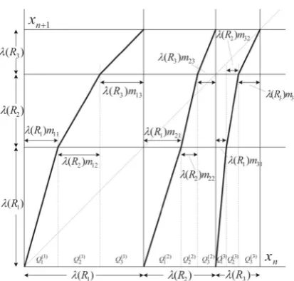
Fig. 1 Construction of 1-D piecewise-linear semi-Markov

trans-formation based on the Frobenius–Perron matrix

Since W₀is non-singular, the Frobenius–Perron matrix

M is given by

M=W₀−1W₁. (30)

The derivative of S|_Q(i)

k

is 1/mi,j, and the length of

Q(_ki)is given by

λQ(_ki)

=q_k(i)−q_k(₋i)₁=mi,jλ(Rj), (31)

which allows computing iteratively q_k(i)for each inter-val Ri starting with q0(i) = ci−1. By assuming each branch S|Ri is monotonically increasing, the

piecewise-linear semi-Markov mapping is given by

S|_Q(i)

k (

x)= 1 mi,j

x−q_k(i₋)₁

+cj−1, (32)

for k=1, . . . ,p(i), and j is the index of image Rjof

Q(_ki); i.e. S(Q(_ki))= Rj, i=1, . . . ,N , j =1, . . . ,N ,

where mi,j =0.

The map is constructed as depicted in Fig.1. In practice, we can choose the piecewise constant probability density functions f₀j(x) = _λ(1_Rj)χRj(x).

These are sampled in order to generate N sets of initial conditions

X0i =

&

x0i_,j

'_θ

j₌1, i =1, . . . ,N, (33)

that will be used in the experiments. For each set of initial conditions Xi₁, we measure a corresponding set of final states

X₁i =

&

x₁i_,j

'_θ

j=1, i =1, . . . ,N, (34)

where x₁i_,j =S(xi_0,k)for some x₀i_,k∈ X₀i. The density function f₁iassociated with the set X₁i of final states is given by

f₁i(x)=

N

j₌1

vi jχRj(x), i =1, . . . , N, (35)

wherevi_,j =_λ(R1 j)·θ

θ

k=1 χRj(x

i

1,k).

Remark We only need to generate initial conditions for

the densities that correspond to the finest uniform parti-tion N=N. Coarser partitions are obtained by merg-ing adjacent intervals, for example Rjand Rj₊1, lead-ing to the new partition{R1, . . . ,RN−1}. It follows that the initial and final states corresponding to the merged interval Rj =Rj∪Rj+1are given by X

j

0=X

j

0∪X

j+1 0 and X₁j = X₁j ∪ X₁j+1, respectively. The initial and final densities corresponding to the merged interval are given by f0j(x) = _λ(1_R¯

J)χRj(x) and f j

1(x) = 1

2λ(Ri)·θ N−1

i₌1

θ

k₌1 χRi(x

j

1,k)χRi(x), respectively.

In general, initial density functions are not piece-wise constant over the partition R. Let f ∈ L2 ⊃ H(RQ), PNQ : _L2 → _H(RQ) _{be the}

orthogo-nal projector operator and ZNQ = I − PNQ such that f = PNQ _f + _ZNQ _f = _f

p + fz. where RQ

= {Q(1) 1 , . . . ,Q

p(1) 1 , . . . ,Q

p(N)

N } = {Q1, . . . ,QNQ},

Ri = ∪_kp₌(i₁)Q_k(i), i = 1, . . . , N , H(RQ) =

span{χ_Q(i)

k }and NQ = N

i=1 p(i).

Theorem 2 A R-semi-Markov, piecewise-linear and expanding transformation, where Ri = ∪_kp₌(i₁)Q(_ki), i =

1, ..,N , can be uniquely identified given a set of initial

densities {f₀i}_iN₌Q₁, NQ = N

i=1

{f₁i}_iN₌₁under the transformation, if{PNQ f₀i}_iN₌Q₁ are linearly independent.

Proof The Frobenius–Perron operator associated with S is given by

PSf0i(x)=

zi=f−1_(x)

f₀i(zi)

|f₀i(zi)|

. (36)

It follows that

f₁i(x)= PSf0i(x)= PSp0i(x)+PSq0i(x)

=

zi=f−1_(x)

pi₀(zi)

|f₀i(zi)|

+

zi=f−1_(x)

q₀i(zi)

|f₀i(zi)|

,(37)

where|f₀i(S|−1

Q(_ki)(x))| ∈ {β1, . . . ., βNQ}.

PNQ f₁i(x)

=PNQPSpi0(x)+PNQPSq0i(x)

=PNQ

i,j:x∈S| Q(_ki)

Q(_ki)

pi₀(S|−1

Q(_ki)(x))

|f₀i(S|−1

Q(_ki)(x))|

+PNQ

i,j:x∈S| Q(i)

k

Q(_ki)

q₀i(S|−1

Q(_ki)(x))

|f₀i(S|−1

Q(_ki)(x))|

. (38)

Then,

PNQ

i,j:x∈S| Q(_ki)

Q(_ki)

q₀i(S|−1

Q(_ki)(x))

|f₀i(S|−1

Q(_ki)(x))|

=

i,j:x∈S| Q(i)

k

Q(_ki)

χ_Q(i) k (x)

βi,k

×

Q(_ki)

q₀i

S|−1

Q(_ki)(x)

dx =0. (39)

Hence,

PNQPSf0i(x)=PSpi0(x)=

NQ

j

w1

i,jχ_Q(j)

k (

x)

=

j_,k_:x_∈S_| Q(_ki)

Q(_ki)

χ_Q(j)

k (

x)

βj,k w

0,j i_,k.

i =1, . . . , NQ. (40)

Alternatively, (27) can be written as

W1=W0MQ, (41)

where MQ =W−₀1W1= {mi,j} NQ

i,j=1is the Frobenius– Perron matrix that corresponds to a unique piecewise linear and expanding transformation S given by

S|_Q(i)

k (x)=

1

ms(i)+1,s(j)+1

x−q_k(i₋)₁

+cj₋1, (42)

for k = 1, . . . ,p(i), j is the index of image Rj of

Q(_ki); i.e. S(Q(_ki))=Rj, i=1, . . . ,N , j=1, . . . ,N ,

s(1)=0 and s(i)=s(i−1)+p(i−1)for i >1.

3.3 Numerical example 1

The applicability of the proposed algorithm is demon-strated using numerical simulation. Consider the fol-lowing piecewise-linear and expanding transformation

S: [0,1] → [0,1]

S|Ri(x)=αi,jx+βi,j, (43)

for i =1, . . . ,4, j = 1, . . . ,4, defined on the parti-tionR = {Ri}4_i=1 = {[0,0.4], (0.4,0.5], (0.5,0.8],

(0.8,1]}, where

(αi,j)1≤i,j≤4=

⎡ ⎢ ⎢ ⎣

10.00 1.25 2.50 1.25 20.00 3.33 15.00 6.67 2.22 1.67 10.00 6.67 10.00 2.50 3.75 5.00

⎤ ⎥ ⎥ ⎦,

(βi_,j)1_≤i_,j_≤4=

⎡ ⎢ ⎢ ⎣

0 0.35 0.20 0.50

−8.00 −1.00 −6.25 −2.33

−1.11 −0.73 −6.90 −4.33

−8.00 −1.70 −2.80 −4.00

⎤ ⎥ ⎥ ⎦.

The graph of S is shown in Fig.2.

A set of initial states X0= {x0,j}θj=1,θ =5×103, generated by sampling from a uniform probability den-sity function f0(x)=χ[0,1](x), were iterated using S to generate a corresponding set of final states XT =

{xT,j}θ_j=1 where T = 20,000. The data set XT was

Fig. 2 Numerical example 1: original piecewise-linear

transfor-mation S

Fig. 3 Numerical example 1: the invariant density estimated

over the initial uniform partition with N=10 intervals

sequence L = {lj}9j=1, lj =10|hj+1−hj|is shown

in Fig.4.

In this example, L= {¯lj}9_j=1= {0.12, 0.18, 0.22,

0.34, 0.40, 0.82, 4.72, 14.32, 15.74}and the mini-mum of

min

lj∈L

⎧ ⎨ ⎩J(R)=

I

fC∗(x)− f_Cd∗_(lj)(x)

2 dx

⎫ ⎬ ⎭, (44)

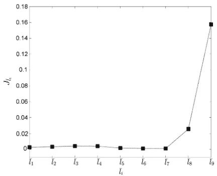
is obtained for l7 = 4.72, as shown in Fig. 5. This corresponds to the final Markov partition R =

Fig. 4 Numerical example 1: the L sequence

Fig. 5 Numerical example 1: the value of the cost function given

in equation (14) for each thresholdl¯j,j=1, . . . ,9.

{R1,R2,R3,R4}, where R1= [0,0.4], R2=(0.4,0.5], R3=(0.5,0.8]and R4=(0.8,1]. Figure6shows the initial density functions used to generate the set of the initial conditions and the final density functions esti-mated from the corresponding final states for T =1.

For the identified partition, the estimated Frobenius– Perron matrix is

M=

⎡ ⎢ ⎢ ⎣

0.1010 0.7900 0.4000 0.8040 0.0500 0.2980 0.0670 0.1510 0.4480 0.6010 0.1020 0.1510 0.1000 0.4020 0.2660 0.2000

⎤ ⎥ ⎥

Fig. 6 Numerical example 1: the initial and final density

func-tions f₀i(x) and f1(i x) corresponding to the identified four-interval partition

Fig. 7 Numerical example 1: the identified transformationS ofˆ

the underlying system

The corresponding identified mapping S is shown inˆ

Fig.7.

The estimated coefficients of the identified piece-wise-linear semi-Markov transformation Sˆ

Ri(x) =

ˆ

αi,jx+ ˆβi,jare

(αˆi,j)1≤i,j≤4=

⎡ ⎢ ⎢ ⎣

9.90 1.27 2.50 1.24 20.00 3.36 14.93 6.62 2.23 1.66 9.80 6.62 10.00 2.49 3.76 5.00

⎤ ⎥ ⎥ ⎦,

Fig. 8 Numerical example 1: relative error between the original

map S and the identified mapS evaluated for 99 uniformly spacedˆ points

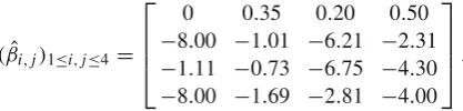
(βˆi,j)1≤i,j≤4=

⎡ ⎢ ⎢ ⎣

0 0.35 0.20 0.50

−8.00 −1.01 −6.21 −2.31

−1.11 −0.73 −6.75 −4.30

−8.00 −1.69 −2.81 −4.00

⎤ ⎥ ⎥ ⎦.

To evaluate the performance of the reconstruction algorithm, we computed the absolute percentage error

δS(x)=100·

S(x)− ˆS(x) S(x)

, (46)

for x ∈ X = {0.01, 0.02, . . . , 0.99}. As shown in Fig.8, the relative error between the identified and original map is less than 2 %. Furthermore, Fig.9shows the true invariant density f∗associated with S super-imposed on the invariant density fˆ∗associated with the identified mapS (Fig.ˆ 7).

In practical situations, measurements are corrupted by noise. Given the process

xn+1=S(xn)+ζn, (47)

where S:R → R is a measurable transformation and {ζn}is a sequence of independent random variables

with density g, it can be shown [41] that the evolution of densities for this transformation is described by the Markov operatorP¯ :L1→L1defined by

¯ P f(x)=

R

Fig. 9 Numerical example 1: the true invariant density (solid

line) and the estimated invariant density (dashed line) of the identified map

Table 1 Reconstruction errors for different noise levels—

example 1

ε=σ2

ε/σx2 0 (noise free) 0.0335 0.1588 0.8819 2.2234

MAPE (%) 0.45 1.14 1.45 8.48 32.30

Furthermore, if P is constrictive then¯ P has a unique¯

invariant density f∗and the sequence{ ¯Pnf}is asymp-totically stable for every f ∈ D [41].

To study how noise affects the performance of our algorithm, we considered the process

xn+1=S(xn)+εζn(mod 1), (49)

where S : [0,1] → [0,1] is a measurable transfor-mation that has a unique invariant density f∗, {ζn}

is i.i.d. with density g andε is a known noise level. This leads to an integral operator P_ε which has a unique invariant density f_ε∗[41]. It can be shown that lim

ε→0Pεf −P f = 0 for all f ∈ D and that, for 0< ε < ε0, if lim

ε→0f ∗

ε exists, then the limit is f∗.

To evaluate the performance of the proposed algo-rithm in the presence of noise, we assumedζ ∼N(0,1) and reconstructed the map for different values ofε. We computed the mean absolute percentage error (MAPE) between S andS.ˆ

δS(x)= 100

θδS

θδS

i=1

S(xi)− ˆS(xi)

S(xi)

, (50)

where{xi}θ_i=δS₁= {0.01, . . . ,0.99},θδS=99.

The results, summarized in (Table1), demonstrate that the algorithm is robust with respect to con-stantly applied stochastic perturbations. Remarkably, the approximation errors remain relatively small even for noise levels that would make it almost impossible to reconstruct the map based on time series data [11,43].

4 Extension to general nonlinear transformations

The approach to reconstructing piecewise-linear and expanding transformations from densities can be extended to more general nonlinear maps. Ulam [44] conjectured that for one-dimensional systems, the infinite-dimensional Frobenius–Perron operator can be approximated arbitrarily well by a finite-dimensional Markov transformation defined over a uniform partition of the interval of interest. The conjecture was proven by Li [45] who also provided a rigorous numerical algo-rithm for constructing the finite-dimensional operator when the one-dimensional transformation S is known. Here, the aim is to construct from data a piecewise-linear semi-Markov transformation S which approxi-ˆ

mates the original map S.

The main assumptions are that (a) S:I → I is

con-tinuous, I = [a,b]; (b) the Frobenius–Perron operator

PS: L1→ L1associated with the transformation has

a unique stationary density f∗and c) P_Snf → f∗for every f ∈ D; i.e. the sequence{P_Sn}is asymptotically stable.

Asymptotic stability of{P_Sn}has been established for certain classes of piecewise C2maps. For example, we have the following result [41].

Theorem 3 If S : [0,1] → [0,1] is a piecewise monotonic transformation satisfying the conditions:

a. There is a partition 0 < c1 < . . . < cN−1 < 1 such that the restriction of S to an interval Ri =

(ci−1,ci)is a C2function;

b. S(Ri)=(0,1);

c. |S(x)|>1 for x =ci;

d. There is a finite constantψsuch that

−S(x)/

(

S(x)

)2

≤ψ, x=ci,i =1, . . . ,N−1,

(51)

By using a change of variables, it is sometimes pos-sible to extend the applicability of the above theorem to more general transformations, such as the logistic map [41], which do not satisfy the restrictive conditions on the derivatives of S.

4.1 Identification of the Markov partition

Although, for a nonlinear transformation, the invariant density f∗∈ D is not piecewise constant, the approach

used to determine the Markov partition for piecewise-linear transformation in Sect.3is also used to determine the optimal partition for the piecewise-linear approxi-mation of the unknown nonlinear map.

4.2 Identification of the Frobenius–Perron matrix

For the identified Markov partition R, a tentative Frobenius–Perron matrix can be identified using the approaches described in Sect.3.

Let the obtained Frobenius–Perron matrix be denoted by Mˆ = (mˆi_,j)1_≤i_,j_≤N. The indices of

the contiguous nonzero entries on the i -the row are denoted by ri = {r_si,r_si +1, . . . ,r_ei}.mˆi,ri

mλ(Rrmi )=

max{ ˆmi_,jλ(Rj)}N_j=1, rmi ∈ ri. Since S is continuous,

∪p(i)

k₌1Rr(i,k) is a connected interval, where Rr(i,k) =

S(Q(_ki)) ∈ R, i = 1, . . . ,N , k = 1, . . . ,p(i); thus, p(i)=rei −rsi+1,{r(i,k)}

p(i)

k=1=ri. Here, r(i,k)∈ {1, . . . ,N}are column indices of nonzero entries on the

i -th row of the Frobenius–Perron matrix which satisfy

r(i,j+1)=r(i,j)+1, (52) for i = 1, . . . ,N, j = 1, . . . ,p(i)−1. This means that mi,r(i,k) > 0 for k = 1, . . . ,p(i)such that the

solution to the optimization problem satisfies

p(i)

k=1

mi,r(i,1)+k−1λ(Rr(i,1)+k−1)=λ(Ri), (53)

and mi,j =0 if j=r(i,k),k=1, . . . ,p(i).

4.3 Reconstruction of the transformation from the Frobenius–Perron matrix

The method for constructing a piecewise-linear approx-imationSˆ(x)over the partitionRis augmented to take

into account the fact that the underlying transformation is continuous and that on each interval of the partition,

SRi is either monotonically increasing or decreasing.

The entries of the positive Frobenius–Perron matrix are used to calculate the absolute value of the slope of

ˆ S|_Q(i)

k as| ˆS|Q( i)

k | = 1/mi,j. A simple algorithm was

derived to decide whether the slope of S|ˆ _Q(i)

k on the

interval Ri is positive or negative.

Let Ii = [cr₍i_,1₎₋1,cr₍i_,p₍i₎₎]for i =1, . . . , N , be

the image of the interval Ri under the transformation

ˆ

S which induce the identified Frobenius–Perron matrix M. cr₍i_,1₎₋1is the starting point of Rr₍i_,1₎which is the image of the subinterval Q(₁i), and c0=a if r(i,1)=1. cr(i,p(i))is the end point of Rr(i,p(i)), the image of the

subinterval Q(_pi₍)_i). As before, {r(i,k)}_kp₌(i₁) denote the column indices corresponding to the nonzero entries in the i -th row of M.

Let ci = 1₂[cr(i,1)−1,cr(i,p(i))]be the midpoint of

the image Ii. The signσ (i)of{ ˆS

(x)

Q(_ki)} p(i)

k₌1is given by

σ (i)=

⎧ ⎨ ⎩

−1, ifc¯i− ¯ci−1<0; 1, ifc¯i− ¯ci−1≥0; σ(i−1), ifc¯i = ¯ci−1,

(54)

for i =2, . . . ,N andσ (1)=σ (2).

Given that the derivative of S|_Q(i)

k

is 1/mi,j, the end

point q_k(i)of subinterval Q(_ki)within Ri is given by

q_k(i)=

⎧ ⎪ ⎪ ⎪ ⎨ ⎪ ⎪ ⎪ ⎩

ci−1+

k

j=1

mi,r(i,j)λ(Rr(i,j)), ifσ (i)= +1;

ci−1+

k

j=1

mi,r(i,p(i)−k+1)λ(Rr(i,p(i)−k+1)), ifσ (i)= −1.

(55)

where k=1, . . . ,p(i)−1 and q(_pi₍)_i)=ci.

The piecewise-linear semi-Markov transformation for each subinterval Q(_ji)is given by

ˆ S_Q(i)

j (x)=

⎧ ⎨ ⎩

1

mi_,j

x−a−q_k(i₋)₁

+cj−1, ifσ(i)=+1;

− 1

mi_,j

x−a−q_k(i₋)₁

+cj, ifσ(i)=−1.

(56)

for i=1, . . . ,N, j =1, . . . ,N,k=1, . . . ,p(i)−1,

Fig. 10 Construction of a piecewise-linear semi-Markov

trans-formation approximating the original nonlinear map

Fig. 11 Numerical example 2: original continuous nonlinear

transformation

The construction of the piecewise-linear semi-Markov transformation to approximate the original continuous nonlinear map is depicted in Fig.10.

A smooth version of the estimated transformation can be obtained by fitting a polynomial smoothing spline.

Fig. 12 Numerical example 2: initial regular histogram based

on a 145-interval uniform partition

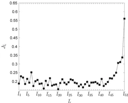
Fig. 13 Numerical example 2: the cost function J_lj, j =

1, . . .,52

4.4 Numerical example 2

The extended reconstruction algorithm is demonstrated using the quadratic (logistic) map (Fig.11)

S(x)=4x(1−x). (57)

It can be shown that{P_Sn}associated with this transfor-mation is asymptotically stable [41].

Fig. 14 Numerical example 2: the invariant density estimated

over on the partitionR= {Ri}72_i=1

{xT,j}θ_j=1where T = 30,000. The data set XT was

used to search for an uniform partition with N intervals, 1 ≤ N ≤ θ/logθ =587, which maxi-mizes the penalized log-likelihood function in Eq. (12), which in this case corresponds to N =145. The esti-mated invariant density f_C∗(x)with respect to the 145-interval partition is shown in Fig.12. In this exam-ple, the longest strictly monotone subsequence L of

L = {lj}144_j=1, lj = 145|h_j+1−h_j| has 52 elements

and the minimization of

Fig. 16 Numerical example 2: reconstructed piecewise-linear

semi-Markov map over the irregular partitionR

min

lj∈L

⎧ ⎨

⎩J(R)=

I

fC∗(x)− f_Cd∗ _(lj)(x)

2 dx

⎫ ⎬ ⎭, (58)

is achieved for l20 = 0.1560, as shown in Fig. 13. This corresponds to a final Markov partition with 72 intervals. The invariant density on the irregular partition

Rwith 72 intervals is shown in Fig.14.

To identify the Frobenius–Perron matrix, 100 den-sities (see Appendix) were randomly sampled to

Fig. 17 Numerical example 2: identified, smooth map

Fig. 18 Numerical example 2: relative error between the original

map S and the identified mapS evaluated for 99 uniformly spacedˆ points

erate 100 sets of initial states X₀i = {xi_0,j}θ_j=1, i = 1, . . . ,100, θ = 5×103. The initial states Xi₀ and their images X₁i under the transformation S were used to estimate the initial and final density functions on

R. Examples of initial and final densities are shown in Fig.15.

The constructed piecewise-linear semi-Markov transformation with respect to the partitionRis shown in Fig.16. The smoothed map, obtained by fitting a cubic spline (smoothing parameter: 0.999), is shown in Fig.17. The relative approximation error is shown in Fig.18.

Fig. 19 Numerical example 2: the true invariant density of the

system (dashed line) and the estimated invariant density of the identified map (solid line) on a uniform partition with 145 inter-vals

Table 2 Reconstruction errors for different noise levels—

example 2

ε 0 (noise free) 0.0206 0.0978 0.5431 1.3692 MAPE (%) 0.61 1.59 2.10 4.42 79.60

The estimated invariant density onR, obtained by iterating the smoothed map 20,000 times with the initial states X0, is shown in Fig.19, compared with the true invariant density [41] f∗(x)=1/π√x(1−x).

The performance of the algorithm for different noise levels was also evaluated, and the results are summa-rized in Table2. As it can be seen, the approximation error remains relatively low (<5 %) for levels of noise (>50 %) that normally cause severe problems to recon-struction algorithms that use time series data.

5 Conclusions

transfor-mation that describes the underlying chaotic dynam-ics. Specifically, the reconstructed maps exhibit the same dynamics as the original systems and therefore can be used to carry out stability analysis, determine invariant sets and manipulate the dynamical behaviour of the underlying system of interest. The applicabil-ity to the proposed methodology and its performance for different levels of noise was demonstrated using numerical simulations involving a piecewise-linear and expanding transformations as well as a continuous one-dimensional nonlinear transformation.

One of the reasons for developing the method pre-sented in this paper was to characterize the hetero-geneity of human embryonic stem cell (hESC) cultures and to develop efficient protocols for controlling their differentiation. In essence, sorted sub-populations of stem cells expressing different levels of particular cell-surface markers can over time reconstitute the equilib-rium distribution of the parent population [46]. Using flow cytometry, it is possible to follow the evolution of the initial density function of the sorted cell frac-tion, by sampling and re-plating cells, over a number of days. The sequence of density functions generated in this process can then be used to infer the under-lying transformation that governs the process, which can help elucidate the existence of cellular substates [47] that, potentially, correspond to the unstable fixed points of the reconstructed map. We have designed the experiments and started generating data by using flow cytometry to sort out cells with different initial densi-ties. These are re-plated and re-analysed in subsequent days to generate sequences of density functions that are required to solve the generalized inverse problem.

The method could be extended to higher-dimensional maps, but this is not necessarily straightforward. The main limitation is the lack of rigorous theoretical results for two- and higher-dimensional maps. While for one-dimensional maps, we have a complete and elegant theoretical framework, for higher-dimensional maps key results are only available for some special cases. A possible solution is to convert the N -dimensional problem to a 1-D problem [29] and esti-mate the corresponding F–P matrix using the approach introduced in this paper. The main challenge is solving the inverse Ulam problem, i.e. construct the transfor-mation based on the estimated F–P matrix. As noted in [30], for higher-dimensional systems Ulam’s con-jecture has been proven only for some special cases [48–51]. The method we are interested to explore to

construct the transformation which approximates the original high-dimensional map is that introduced by Bollt [30].

Acknowledgments X. N. gratefully acknowledges the support

from the Department of Automatic Control and Systems Engi-neering at the University of Sheffield and China Scholarship Council. D. C. gratefully acknowledges the support from MRC, BBSRC and the Human Frontier Science Program.

Open Access This article is distributed under the terms of the

Creative Commons Attribution License which permits any use, distribution, and reproduction in any medium, provided the orig-inal author(s) and the source are credited.

6 Appendix: initial states for example 2

The 100 sets of initial states used in example 2 are obtained by sampling the following density functions:

fβ1

0,1(x, β1)= 7 10·

x29(1−x)β1−1 B(30, β1)

+ 3

10·

xβ1−1(1−x)29

B(β1,30) , β1=1, 2, . . . , 30;

fβ2

0,2(x, β2)=

xβ2−1(1−x)29

B(β2,30) , β2=1, 2, . . . , 25;

fβ3

0,3(x, β3)=

x29(1−x)β3−1

B(30, β3) , β3=1, 2, . . . , 25;

fβ4

0,4(x, β4)= 1 2 ·

x39(1−x)β4+19

B(40, β4)

+1

2 ·

x39(1−x)β4+19

B(40, β4) , β4=1, 2, . . . , 10;

fβ5

0,5(x, β5)= 1 2 ·

xβ5+19(1−x)39

B(β5,40)

+1

2 ·

xβ5+19(1−x)39

B(β5,40) , β5=1, 2, . . . , 10; where B(·, ·)is beta function.

References

2. Coen, E.M., Gilbert, R.G., Morrison, B.R., Leube, H., Peach, S.: Modelling particle size distributions and secondary parti-cle formation in emulsion polymerisation. Polymer 39(26), 7099–7112 (1998). doi:10.1016/S0032-3861(98)00255-9

3. Wang, H., Baki, H., Kabore, P.: Control of bounded dynamic stochastic distributions using square root models: an applica-bility study in papermaking systems. Trans. Inst. Meas. Con-trol 23(1), 51–68 (2001)

4. Mondragó, R.J.C., : A model of packet traffic using a random wall model. Int. J. Bifurc. Chaos 09(07), 1381–1392 (1999). doi:10.1142/S021812749900095X

5. Rogers, A., Shorten, R., Heffernan, D.M.: Synthesizing chaotic maps with prescribed invariant densities. Phys. Lett. A 330(6), 435–441 (2004). doi:10.1016/j.physleta.2004.08. 022

6. Wigren, T.: Soft uplink load estimation in WCDMA. IEEE Trans. Veh. Technol. 58(2), 760–772 (2009). doi:10.1109/ tvt.2008.926210

7. Farmer, J.D., Sidorowich, J.J.: Predicting chaotic time series. Phys. Rev. Lett. 59(8), 845–848 (1987)

8. Casdagli, M.: Nonlinear prediction of chaotic time series. Physica D 35(3), 335–356 (1989). doi:10.1016/ 0167-2789(89)90074-2

9. Abarbanel, H.D.I., Brown, R., Kadtke, J.B.: Prediction and system identification in chaotic nonlinear systems: time series with broadband spectra. Phys. Lett. A 138(8), 401– 408 (1989). doi:10.1016/0375-9601(89)90839-6

10. Principe, J.C., Rathie, A., Kuo, J.-M.: Prediction of chaotic time series with neural networks and the issue of dynamic modeling. Int. J. Bifurc. Chaos 02(04), 989–996 (1992). doi:10.1142/S0218127492000598

11. Aguirre, L.A., Billings, S.A.: Identification of models for chaotic systems from noisy data: implications for perfor-mance and nonlinear filtering. Physica D 85(1–2), 239–258 (1995). doi:10.1016/0167-2789(95)00116-L

12. Billings, S.A., Coca, D.: Discrete wavelet models for iden-tification and qualitative analysis of chaotic systems. Int. J. Bifurc. Chaos 09(07), 1263–1284 (1999). doi:10.1142/ S0218127499000894

13. Lueptow, R., Akonur, A., Shinbrot, T.: PIV for granular flows. Exp. Fluids 28(2), 183–186 (2000)

14. Wu, J., Tzanakakis, E.S.: Deconstructing stem cell pop-ulation heterogeneity: single-cell analysis and modeling approaches. Biotechnol. Adv. 31(7), 1047–1062 (2013). doi:10.1016/j.biotechadv.2013.09.001

15. Friedman, N., Boyarsky, A.: Construction of Ergodic trans-formations. Adv. Math. 45(3), 213–254 (1982)

16. Ershov, S.V., Malinetskii, G.G.: The solution of the inverse problem for the Perron–Frobenius equation. USSR Comput. Math. Math. Phys. 28(5), 136–141 (1988)

17. Góra, P., Boyarsky, A.: A matrix solution to the inverse Perron–Frobenius problem. Proc. Am. Math. Soc. 118(2), 409–414 (1993)

18. Diakonos, F.K., Schmelcher, P.: On the construction of one-dimensional iterative maps from the invariant density: the dynamical route to the beta distribution. Phys. Lett. A

211(4), 199–203 (1996)

19. Pingel, D., Schmelcher, P., Diakonos, F.K.: Theory and examples of the inverse Frobenius–Perron problem for com-plete chaotic maps. Chaos 9(2), 357–366 (1999)

20. Huang, W.: Constructing chaotic transformations with closed functional forms. Discret. Dyn. Nat. Soc. 2006, 1–16 (2006)

21. Huang, W.: On the complete chaotic maps that preserve pre-scribed absolutely continuous invariant densities. In: Topics on Chaotic Systems: Selected Papers from CHAOS 2008 International Conference, pp. 166–173 (2009)

22. Huang, W.: Constructing multi-branches complete chaotic maps that preserve specified invariant density. Discret. Dyn. Nat. Soc. 2009, 14 (2009). doi:10.1155/2009/378761

23. Boyarsky, A., Góra, P.: An irreversible process represented by a reversible one. Int. J. Bifurc. Chaos 18(07), 2059–2061 (2008)

24. Baranovsky, A., Daems, D.: Design of one-dimensional chaotic maps with prescribed statistical properties. Int. J. Bifurc. Chaos 5(6), 1585–1598 (1995)

25. Diakonos, F.K., Pingel, D., Schmelcher, P.: A stochas-tic approach to the construction of one-dimensional chaotic maps with prescribed statistical properties. Phys. Lett. A 264(2–3), 162–170 (1999). doi:10.1016/ S0375-9601(99)00775-6

26. Koga, S.: The inverse problem of Flobenius–Perron equa-tions in 1D difference systems-1D map idealization. Prog. Theor. Phys. 86(5), 991–1002 (1991)

27. Rogers, A., Shorten, R., Heffernan, D.M.: A novel matrix approach for controlling the invariant densities of chaotic maps. Chaos Solitons Fractals 35(1), 161–175 (2008). doi:10.1016/j.chaos.2006.05.017

28. Berman, A., Shorten, R., Leith, D.: Positive matrices asso-ciated with synchronised communication networks. Linear Algebra Appl. 393, 47–54 (2004). doi:10.1016/j.laa.2004. 07.016

29. Rogers, A., Shorten, R., Heffernan, D.M., Naughton, D.: Synthesis of piecewise-linear chaotic maps: invariant den-sities, autocorrelations, and switching. Int. J. Bifurc. Chaos

18(8), 2169–2189 (2008)

30. Bollt, E.M.: Controlling chaos and the inverse Frobenius– Perron problem: global stabilization of arbitrary invariant measures. Int. J. Bifurc. Chaos 10(5), 1033–1050 (2000) 31. Lozowski, A.G., Lysetskiy, M., Zurada, J.M.: Signal

processing with temporal sequences in olfactory systems. IEEE Trans. Neural Netw. 15(5), 1268–1275 (2004). doi:10. 1109/tnn.2004.832730

32. Pikovsky, A., Popovych, O.: Persistent patterns in determin-istic mixing flows. Europhys. Lett. 61(5), 625 (2003) 33. Wyk, M.A.v., Ding, J.: Stochastic analysis of electrical

cir-cuits. In: Chaos in Circuits and Systems, pp. 215–236. World Scientific, Singapore (2002)

34. Isabelle, S.H., Wornell, G.W.: Statistical analysis and spec-tral estimation techniques for one-dimensional chaotic sig-nals. IEEE Trans. Signal Process. 45(6), 1495–1506 (1997) 35. Götz, M., Abel, A., Schwarz, W.: What is the use of Frobenius–Perron operator for chaotic signal processing? In: Proceedings of NDES. Citeseer (1997)

36. Altschuler, S.J., Wu, L.F.: Cellular heterogeneity: do dif-ferences make a difference? Cell 141(4), 559–563 (2010). doi:10.1016/j.cell.2010.04.033

38. Schütte, C., Huisinga, W., Deuflhard, P.: Transfer operator approach to conformational dynamics in biomolecular sys-tems. In: Fiedler, B. (ed.) Ergodic Theory, Analysis, and Efficient Simulation of Dynamical Systems, pp. 191–223. Springer, Berlin (2001)

39. Potthast, R.: Implementing Turing Machines in Dynamic Field Architectures. arXiv preprintarXiv:1204.5462(2012) 40. Boyarsky, A., Góra, P.: Laws of Chaos: Invariant Measures and Dynamical Systems in One Dimension. Probability and its Applications. Birkhäuser, Boston, MA (1997)

41. Lasota, A., Mackey, M.C.: Chaos, Fractals, and Noise: Sto-chastic Aspects of Dynamics, 2nd edn. Springer, New York (1994)

42. Rozenholc, Y., Mildenberger, T., Gather, U.: Combining regular and irregular histograms by penalized likelihood. Comput. Stat. Data Anal. 54(12), 3313–3323 (2010). doi:10. 1016/j.csda.2010.04.021

43. Aguirre, L.A., Billings, S.A.: Retrieving dynamical invari-ants from chaotic data using NARMAX models. Int. J. Bifurc. Chaos 05(02), 449–474 (1995). doi:10.1142/ S0218127495000363

44. Ulam, S.M.: A Collection of Mathematical Problems: Inter-science Tracts in Pure and Applied Mathematics, vol. 8. Interscience, New York (1960)

45. Li, T.-Y.: Finite approximation for the Frobenius– Perron operator. A solution to Ulam’s conjecture. J. Approx. Theory 17(2), 177–186 (1976). doi:10.1016/ 0021-9045(76)90037-X

46. Chang, H.H., Hemberg, M., Barahona, M., Ingber, D.E., Huang, S.: Transcriptome-wide noise controls lineage choice in mammalian progenitor cells. Nature 453(7194), 544–547 (2008)

47. Enver, T., Pera, M., Peterson, C., Andrews, P.W.: Stem cell states, fates, and the rules of attraction. Cell Stem Cell 4(5), 387–397 (2009)

48. Froyland, G.: Finite approximation of Sinai–Bowen–Ruelle measures for Anosov systems in two dimensions. Random Comput. Dyn. 3(4), 251–264 (1995)

49. Froyland, G.: Computing physical invariant measures. In: International Symposium on Nonlinear Theory and its Applications, Japan, Research Society of Nonlinear Theory and its Applications (IEICE), pp. 1129–1132 (1997) 50. Boyarsky, A., Lou, Y.: Approximating measures

invari-ant under higher-dimensional chaotic transformations. J. Approx. Theory 65(2), 231–244 (1991)