Calculation of the time averaged optical transfer function by the fast Fourier transform

Rochester Institute of Technology

RIT Scholar Works

Theses

Thesis/Dissertation Collections

6-1-1976

Calculation of the time averaged optical transfer

function by the fast Fourier transform

Jan Pierce

Follow this and additional works at:

http://scholarworks.rit.edu/theses

This Thesis is brought to you for free and open access by the Thesis/Dissertation Collections at RIT Scholar Works. It has been accepted for inclusion in Theses by an authorized administrator of RIT Scholar Works. For more information, please [email protected].

Recommended Citation

MASTER

I

S THESIS

This is to certifY that the Master's Thesis of

Jan L. Pierce

name of student

yjt.b

a

maJor in

»

date

John F. Carson

Thesis Committee:

~~~~~~

_ _ _

_

Thesis adViser

G. W. Schumann

Graduate adviser

CALCULATION OF THE TIME AVERAGED

OPTICAL TRAwSFER FUNCTION

BY THE FAST FOURIER TRANSFORM

by

Jan L. Pierce

A thesis submitted in partial fulfillment of the

requirements for the degree of Master of Science in Photographic Science and Instrumentation

at the Rochester Institute of Technology.

ACKNOWLEDGMENT

The author expresses his gratitude to his thesis advisor, Pro fessor John F. Carson of the Department of Photographic

Science,

Rochester Institute of

Technology

for his patience and guidance. In

particular the author extends his appreciation to Barbara Friedman and Carol

Lindsey

of the Office of Computer Services for their assistance

with the Tektronix graphics routines and in

learning

to use the Xerox Sigma

6

_software,

hardware,

and shared processors.

In addition the author would like to thank Mr. Peter Engeldrura of the Xerox Webster Research Center for several _enlightening dis cussions _{relating to} two-dimensional Fourier

transforms,

and Mr. B. R. Desai of RIT for _contributing the 16mm shutter film.

Finally

the author _gratefully acknowledges the support of the United States Central Intelligence

Agency

which enabled the author to use state-of-the-art computer graphics software.

TABLE OF CONTENTS

LIST OF FIGURES iv

I.

INTRODUCTION

1

II. THEORY

3

III.

PROCEDURE

23

IV.

RESULTS 31

V. SUMMARY

68

REFERENCES . 7h

GENERAL REFERENCES ... 76

APPENDIX A

80

APPENDIX B

89

APPENDIX C 92

APPENDIX D

9$

APPENDIX E 98

APPENDIX F 112

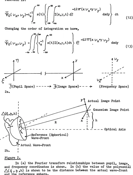
Figure 1. A schematic representation of the process

leading

to image formation on photographic

film.

Figure

2.

In

(a)

the Fourier transform relationships _{between pupil,}

image,

and

frequency

coordinates is shown. In

(b)

the value of the polynomial

^Mf

>^*h) is shown to be the distance

between the actual wave-front and the reference sphere.

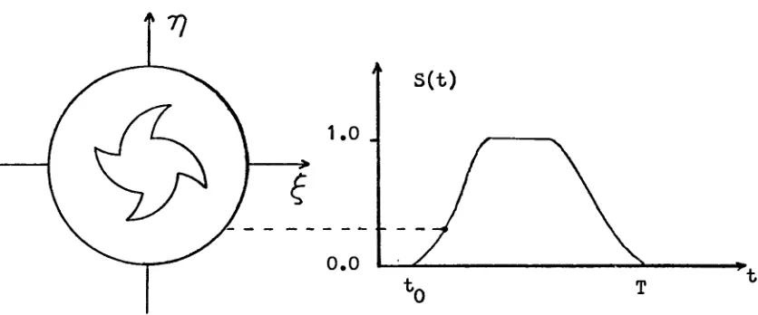
Figure

3.

The blades of a certer _opening pupil shutter form a pinwheel or bent star shape

during

_exposure, and

the"

shutter function

S(t)

is used to weight the _{corresponding two-dimensional} OTF.

Figure

U.

A two-dinensional _{array representing} a circular pupil function sampled at frequencies

T~

and

T~.

x _y

Figure

5*

A graphical development of the discrete Fourier transform.

Figure

6.

Graphical development of the discrete Fourier

transform,

continued from Figure 5-

Sampling

the function F'

(v)

to obtain

F(n)

makes f

'(k)

periodic in the space donain.

Figure 7.

Aliasing

occurs when the DFT is applied to functions which are not

band-limited,

and the

frequency

labeled i/is known as the Nyquist or

folding

frequency.

Figure

8.

When aliasing occurs, high frequencies are detected

by

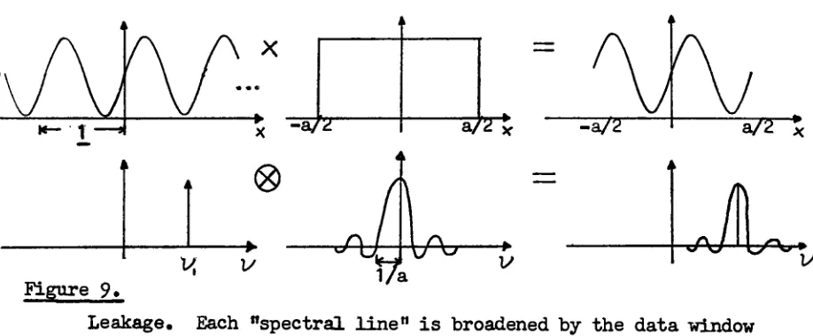
the sampling process as low frequencies.

Figure 9. Leakage. Each "spectral line"

is broadened

by

the data window sine function.

Figure

10.

The

frequency

response of the DFT is not

flat,

but contains a rdpple due to the finite mimber of data points.

Figure

11.

A schematic representation of the relation between the discrete and continuous quantities.

Figure

12.

The location of _{the unity} amplitude data window in

one-dimension.

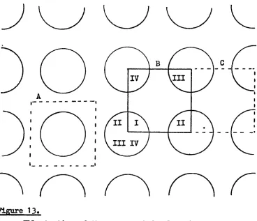
Figure 13. Illustration of the proper window location in kx- k _space for a function defined on a circular region. y

Figure .k. The proper locations of the function quadrants in the transform array.

Figure

16.

Outline of the algorithm used in the main program 0TF2D.

Figure

17.

Outline of the algorithm used in the main program 0TF2D continued from figure

16.

Figure

18.

The shutter functions

S(t)

and

S(t.).

Figure

19.

The OTF for a diffraction limited optical system as calculated

by

the FFT program 0TF2D and compared to the theoretical values.

Figure

20.

Absolute error in the diffraction limited OTF _using the

theoretical

results as reference.

Figure

21.

OTF for a circular exit pupil and one wave of defocus.

Figure

22.

The OTF for a circular exit pupil and

1/TTwaves

of defocus.

Figure

21;.

The absolute difference between the time-averaged diffraction limited OTF as calculated

by

_{the FFT} program _{0TF2D using} values

calculated from the analytical solution in equation 31 as

reference.

Figure

2$.

The two-dimensional diffraction limited OTF for a circular

exit pupil.

Figure

26.

The two-dimensional diffraction limited OTF for one of the frames used in the leaf shutter model.

Figure 27- The time-averaged two-dimensional diffraction limited OTF

for the leaf shutter model.

Figure 28. The two-dimensional OTF for a circular exit pupil and one

wave of defocus.

Figure 29. The two-dimensional OTF for one frame of the leaf shutter

model and one wave of defocus.

Figure 30. The two-dimensional time-averaged OTF for the leaf shutter

model and one wave of defocus.

Figure 31. The time-averaged diffraction limited OTF.

Figure 32. The time-averaged OTF for

1/U

wave of

defocus.

Figure

33.

The time-averaged OTF for 1/2 wave of

defocus.

Figure 3b. The time-averaged OTF for one wave of

defocus.

Figure 3$. The difference between the valuse predicted

by

the leaf shutter and circular shutter models for an aberration-free

Figure 37. The time-averaged OTF at

Wvc

-

0.25

_{for the leaf shutter} model as a function of the defocus coefficient 0C20

Figure

38.

The time-averaged OTF for one wave of third order spherical

aberration.

Figure 39. The difference between the values predicted

by

the leaf

shutter and circular shutter models for one wave of third order shperical aberration.

Figure

UO.

The _{relationship between the wave-front,}

l

max*, and

$.

Figure

U1.

The time-averaged OTF at the optimum focus position

(jLL=.8)

for an optical system with both third and fifth order

spherical aberration.

Figure

U2.

The figures

U2(a)

-

(i)

_show the _{effect of}

defocusing

_a

fully-corrected optical system on the time-averaged OTF for the leaf shutter

(+)

and on the system OTF with the shutter removed

(

).

Figure

U3.

Comparison of the Leaf Model and Circular Model Shutter Functions,

Figure

hh.

The effect on defocusion a

fully

corrected optical system

on the OTF at

V/v

= .2$.

ABSTRACT

The fast Fourier transform is used in two-dimensions to calculate _{the apodizing} effect of a center _opening

pupil shutter. Two shutter models are investigated and

compared, a circular shutter with diameter a function

of

time,

and a five-bladed leaf-type shutter. The influence of shutter _shape,

defocus,

and third and

fifth order spherical aberration on the time-averaged

optical transfer function is investigated. The results indicate that _{there is only} a small effect on resolution

and depth of focus due to shutter motion in a well

The optical transfer function

(OTF)

of a lens may be calculated

from the pupil function

by

_performing two Fourier transforms.

Assuming

a point _object,

transforming

the pupil function

(,7])

yields the

amplitude spread function a(x,y). The OTF for incoherent light is

then the Fourier transform of the

intensity

spread function

I(x,y)

-a(x,y) a*(x,y).

*

A center _opening pupil shutter changes the shape of the exit

pupil,

and hence the

OTF, during

exposure. This

implies,

_providing

reciprocity

holds,

and in the absence of image _motion, that the

effective photographic transfer function is the result of a

time-averaged apodization. In

1959 Bechtel(1)

investigated the effect

of a _{slowly opening} "between-the-lens" circular shutter on resolution

by

calculating the spread function.

Shack(2)

in

196U

also assumed

a circular shutter and for a shutter _efficiency of

fifty

percent

indicated the effect of defocus on the time-averaged OTF. An ex

amination of the available literature reveals no evidence of

experiments in which the Fourier transform is applied in two dimen

sions in order to predict the effect of shutter motion on image

quality.

Efficient evaluation of the Fourier transform became possible

with the development of an algorithm in

1965 by

James W.

Cooley

and John W. Tukey(3). Use of the _{algorithm, known} as a "fast"

Fourier transform

(FFT),

reduces the number of machine calculations

algorithm has been used _successfully

by

Lerman(li)

in 1968 to evaluate

the effect of third order spherical aberration on the two-dimensional

OTF,

by

Minnick and

Rancourt(5)

in 1968 for "real"

optical systems

with and without central

obscurations,

and

by Baum(6)

in 1972 to calcu

late third and seventh order spherical aberration. It has been suggest

ed that the OTF _may be calculated _{for any} image _{point, lens aberrations,}

and aperture shapes _using this technique.

The purpose of this research is to create a.computer program

which will calculate the time-averaged OTF which results when the

exposure is made with a center _opening pupil shutter. The effects

of shutter _shape,

defocus,

and spherical aberration on the

time-averaged OTF will be

investigated,

and the results used to examine

Providing

reciprocity

holds,

the

of _energy received in the image of a pnotographic system is equal

to the time-integrated optical image. The optical _{image may vary}

during

exposure due to image _motion, which has been treated in re

ferences

7-10 _, and due to shutter _motion, which changes the shape

of the exit pupil.

Assuming linearity

and _{stationarity,} Fourier

analysis ana transfer _{functions may} be used to cHaracterize the

system _up to the formation of the exposure

image,

a hypothetical

image in terms of energy rather than power per unit area. The sta

tistical _{latent image may} then be obtained

by

a non-linear

transi"er(

₁₁

)m

R. V.

Shack(12)

has shown that the effective photographic trans

fer function associated with the exposure _{image may be} written as:

co

-oo

Where,

1/ _, i/ Spatial

frequency

coordinates

x _y

Tp

= Transfer function associated witn the film

t - _{Effective exposure time}

s(t) Shutter function

^aYq(

fx> Vyt^) = _{The time dependent optical transfer}

function

x(tj,y(tj = _{Parametric expressions}

describing

image

In the absence of image motion equation

(1)

becomes:

/-oo

"*E- Vx

*y>

"%*?

/

-*>%( Vx

V

t)

dt

-oo

(2)

[OPTICAL

IMAGE

Variation in time due to shutter motion

Variation in time

due to image motion

/

I

EXPOSURE IMAGE

Distribution of

photographic grains

LATENT IMAGE

LINEAR TRANSFER

NON-LINEAR TRANSFER

Figure 1.

^E

=

Wo

(3)

where,

oo

-1

-oo

is the time-averaged optical transfer function.

The optical _{transfer function may be} obtained from the pupil

function

by

_{performing two Fourier} transforms.

Assuming

a point

object,

transforming

the pupil function

P(,77t)

Proc-Uces the

amplitude spread function:

(U)

a(x,y,t) =

.00 00

n^v^)e

-**

d^

(5)

-00 -00

The OTF for incoherent light is then the Fourier transform of the

intensity

spread

function,

00 00

I(x,y,t)e"i2'n"(xl/x^^y)dxdy

(6)

where,

I(x,y,t)

= _{a(x,y,t)a*(x,y,t)}

The pupil

function,

which describes the shape of the wave-front

emerging from the exit pupil

(figure

2b.),

_may be written _as,

p(f.77.t)-i(f.77.t)e12,rA<f,?'h)

(8)

where

A(r,77,t)

represents the amplitude transmittance of the exit

pupil and

Z\(>77h)

is a polynomial which describes the aberrations

present

(13).

The relationships _{between the pupil, the}

image,

and the

frequency

coordinate systems are shown in figure 2.

With an appropriate change to polar coordinates

(1U)

the aberration

polynomial

becomes,

A(p,0,h)

-oC00 +

(oC20/2+1C11hPCos(+2COOh2)

2_2

2 + (0CliOpSC31hp3 Cos<+2C22h2p2Cos

+ + 3C11h3pCos<fc> +

^^

)

?

and

looking

at a point on the optical _axis,

A(p,<f>,o)

=

0c00 +

+ * ?

(9)

(10)

a polynomial in powers of O in which the value of the coefficients

0C20 0CliO 0C60 ' determine the amount of

defocus,

third and fifth

order spherical aberration present in the image.

Considering

on axis points and _{up to fifth} order spherical

aberration, the amplitude spread function is then given by:

J

J

(11)

-1

%lVxVy)<l

S(t)<

.00 _ _oo

I(x,y,t)

-27r(xl/y+y\yy)

dxdy

}

dt

^-00 -OO

Changing

the order of integration we

have,

(12)

00

At oo

-1

NM^x,Vy)

-<t~'

s(t)l(x,y,t)dt

>e

-i2TT(x _i/x+yyy)

-00 -Ck> _oo

f

7?

dxdy

?

!-.

(13)

-5

5-Hf

j(Pupil

Space)

*

J

(Image Space)

>

(Frequency

Space)

2a.

A($,*,-0

-Reference

(Spherical)

Wave-Front

T"

Actual Wave-Front 2b.

y

\

Actual Image Point

Gaussian Image Point

h

- Optical Axis

Figure 2.

In

(a)

the Fourier transform relationships between _pupil,

image,

and

frequency

coordinates is shown. In

(b)

the value of the polynomial

/\(

E _, % ,h) is shown to be the distance between the actual wave-front [image:16.551.50.505.101.698.2]

or.

oo ao

Y0(^x>i/y)

-I

fi-^y-

e

-i2TT(x1/ _+yi/v)

dxdy

(1U)

-oo-oo

where

T(x,y)

is the time-averaged

intensity

spread function.

Now consider the operation of a center _opening pupil shutter

during

a short exposure. The amplitude transmittance of the exit pupil

is modified

by

the motion of the shutter blades _as,shown in figure 3.

If we assume the shutter allows a transmittance of 1 .0 or

0.0,

the

effect of the _changing shutter shape _may be included in the

A(rt7^Jt)

term.

;'

S(t)

Figure 3.

The blades of a center _opening pupil shutter form a pinwheel

or bent star shape

during

_exposure, and the shutter function

S(t)

is used to weight the corresponding two-dimensional OTF.

For evaluation on a digital computer

A(g,7^,t),

_a(x,y,t), and [image:17.551.62.480.351.525.2]

The pupil function is then defined

by

a two-dimensional _array of _points,

and the continuous Fourier

transform,

7

/

-i27T( i/y. + i^y)

p<^

V

Jf(^'e

dxd-

(1S)

becomes the discrete Fourier transform:

V1

*?

-i2ir(nxk3C/hx + nyky/Ny)

^x^VVW

=

,4

X

h(kxTx-

Vy}

e

where, nx=0,1,2,...,Nx-1 and ny=0,1 ,2,...,Ny-1

(16)

The function f

(x,y)

is sampled at frequencies

T~

and such

that x-k _T and y-le.T where

1^

and

k^

are integers between zero and

Nx

and Ny.

U

^

N oooooooooooooooo o

oooooooooooooooo o

oooooooooooooooo o

oooooooooooooooo o

ooooooeooooo o i

~y

OOOOO09**OOOO o oooo*****ooo o ooo*t>oo o ooo**oo o ooo***oo o ooo*oo o ooo***oo o ooootooo o

. ooooooooo o

*

oooooo*****ooooo o

3

oooooooooooooooo o

2 oooooooooooooooo o

1 oooooooooooooooo o

V

1 2 3...

*

Nx

Fifflire

U.

A two-dimensional array representing a circular pupil function

sampled at frequencies T~

and T

10

The graphical development of a one dimensional discrete Fourier

transform

(DFT)

in figures

5

and

6,

will

help

to illustrate the three

problems known as _aliasing,

leakage,

and the picket-fence _effect, which

arise when equation

(16)

is substituted for equation

(15).

The function to be

transformed,

f(x),

is multiplied

by

a comb

of delta functions and

by

a _unity amplitude data-window to obtain

the

finite,

discrete

function,

f(k). Since multiplication in the space

domain corresponds to convolution in the

frequency

domain,

the transform

of

f(k)

is the result of _convolving

F(l/)

with another comb of delta

functions and then with a sine function due to the data window. When

the resulting periodic function

F'(v)

_{is sampled, the function}

f-(k)

is made periodic

(figure

6).

Both functions of the discrete Fourier transform pair f (k)

F(n)

are _periodic, and if

f(x)

is not band

limited,

F(i/)

will not be finite

and _{overlapping in}

F(n)

will occur

(figure

7) The overlapping is

referred to as

aliasing,

and will always occur to some extent unless

the space function is band

limited.

In that case it is prevented

by

-1

making the sampling

frequency

T at least twice the highest

frequency

component present in f

(x)

(the

function f

(x)

shown in figures

5

and

6

is band

limited)

. The _aliasing which occurs with non-band limited

-P cd 0) p CD O CO H fc ---T)

<D>_"EJ

Eh - 3

P w CD Si o rt g a o H -P U <H 0) CO u * cd cu .0 ,fl -P

Ik

II

-l*

OJ 0 En CM 0 c:> E-t 1 . "ti <rt cv o c TJ G r-i

. O (X U aj rt

a> +> -p a

S o o >

3 -H-P

C CO r-l -H O

H P. fl TJ

P W -P -H H CD H cd ?

fl i-H 3

rt Q. g J3 cd

*h e -p-p

< W X>

^S

TJ

0 T > O fl U) 2 o d) fn 4H fl H n> cd -3 e-p 0 T) c H CD O fl cd O fX-rt m -p 73 IDt-i X! P -p t> fl c O H O fl O O -P H -P 10 cd tJ 0 fl H O H P. P. 0J H CD -P U

g

UO a O JL. fc S -P 0 0 fc . CD O Xi

rt cd P

fc fc O

SS

O ti _fc

ed (D CD -3

J5 <H -P En O O

F(V)

Figure 7.

Aliasing

occurs when the DFT is applied to functions which are not

band-limited,

and the

frequency

labeled

V

is known as the Nyquist

or

folding

frequency.

'IfAl/

V,

Vfr&V

Figure

8.

When aliasing occurs, high frequencies are detected

by

the [image:22.551.32.509.99.563.2]

1U

The problem of leakage is caused

by

_analyzing a finite number

of data points. Consider an input consisting of _only one

frequency

l/i

(figure

9). Multiplication

by

a finite data window broadens the

delta function

by

convolution with a sine function. The contribu

tion of Va. to a spectrum would leak via the side lobes of the sine

function into other frequencies.

According

to

Bergland(l5)

the side

lobes and hence leakage may be reduced

by

_applying data windows which are not rectangular.

A

i

A

A

X

\

J

\J\

A

**

* 1

J

X

[image:23.551.43.502.264.454.2]

M

Figure 9.

Leakage. Each "spectral line" _{is broadened}

by

the data window

sine function.

The picket-fence effect is also caused

by

the finite data

window. The

frequency

response of the DFT might be represented

by

the plot in figure

10.

The response at each of the out-put fre

quencies

(multiples

of T~

)

is not

rectangular,

rather it has the

shape of the main lobe of the sine function shown in

figure

nine. A

frequency

component 1/'_, betweenV, and

1/h,

is detected

by

both the

fourth and fifth harmonic windows, but with a response of less than

analogous to viewing the true spectrum through a picket fence. The

effect is reduced when the width of the main lobe is

increased,

that

is,

by

applying a non-rectangular data _window, or

by

_{extending the}

length of the data window with a set of zero valued samples. The

last of these two solutions produces frequencies between the original

harmonics.

DFT

Response

1.0-1 2

3

Harmonic Number Figure 10.

The

frequency

response of the DFT is not

flat,

but contains

a ripple due to the finite number of data points.

The problems of _aliasing and leakage encountered in OTF

calculations are discussed

by Lerman(l6)

and Minnick(17).

Aliasing

may be prevented

by

_calculating the OTF cut-off

frequency

_\y for

a circular exit pupil. Consider in one dimension the relationships

between the discrete and continuous quantities _{in the transforms from}

pupil space

(f,Tj)

to image space

(x,y),

and then to

frequency

space

16

v*

.-,y

Pupil Coordinates

(,77)

(Vx'VV

Image coordinates

U,y)

(7-s

A

T,

,n9

A^

I,

)

(nx/NxTx>Wy)

Frequency

coordinates

(

l/X,

l/y)

Figure 1 1.

A Schematic representation of the relation between the discrete

and continuous quantities.

We have

that,

t-H\

07)

x = _{k T}

x x

and when we compare the quantities in the exponentials of

equations

(11)

and

(16),

08)

X a

X

f

or _substituting equation

(17)

:

(19)

x ==

^R

nE nc -"0,1,2,... N. -1

T?N^

(20)

The cut-off

frequency

for a circular exit pupil _may be written

as,

'e.x- _2max

and in order to prevent _{aliasing in}

frequency

_space,

f1 _s

2 y

x c

or:

T -

X

_R

x

T

^

max

(22)

Substituting

equation

(22)

into

(18),

X

R

;max

x =

kx

y

*

kx

- _0,1,2,.

..Nx-1

(23)

eliminating x between

(20)

and

(23),

k ^=0,1,2,..^-!

m

*

^max

n

=0,1,2,...N?-1

(2U)

and with

Nx

= _{N we have:}

fJ

-

af

%

s

N4

(25)

Assuming

then that the cut-off

frequency

is given

by

equation

(21),

sampling the pupil function at the

frequency

T will prevent

aliasing of the OTF results. Note also from equation

(25),

_{that if}

the pupil function is represented

by

an _array of 32 x 32 elements

(C

m ₁₆

),

then a

6U

x

6k

array must be presented to the DFT as

input.

18

be concentrated in a small area

(due

to aberrations and _possibly the

shutter effect under

investigation),

leakage will occur when it is

truncated to an N X N array. As stated _previously, the error due

x _y

to

leakage

and the picket-fence _effect, may be reduced

by increasing

the number of data points N ,N

(and

thus

N>

,N

)

in the transform.

The problem of _accuracy versus the number of data points is investigated

by

Baum(l8).

Also of importance in

defining

the input data to a discrete

Fourier transform is the definition of the function value at a point

of discontinuity. A sufficient but not _necessary condition for the

existence of a Fourier transform

F(l/)

is that

f(x)

is integrable

in the sense

that,

.00

|

f

(x)

|

dx < oo

loo

However,

if f

(x)

is a periodic or an impulse

function,

justification

of the existence of

F(t/)

requires the use of distribution

theory

as

indicated

by

Brigham(19). Distribution

theory

indicates _{that any func}

tion f

(x)

must be defined as the mid-value at points of

discontinuity

in order for a unique inverse transform to exist.

p

When the pupil function is defined

by

an _array of N

elements,

evaluation of the discrete Fourier transform in equation 16 requires

N^

complex multiplication-addition _operations. The fast Fourier

and _{John W.}

Tukey(20)

in

1965

makes use of the periodic properties of

the complex exponential kernel to reduce the number of calculations.

In

particular,

if all the factors of N and N are equal to

2,

that

is,

x _y

Nx-N

2^, the number of operations is reduced to

IjN

LogJJI. A reduction

from

16,777,216

to

98,30a

complex multiplication-additions is obtained

for a

6a

x

6a

_working array.

Significant in the processing of data with the fast Fourier

transform is the location of _{the unity} amplitude data window. In

the one-dimensional case the FFT algorithm assumes that the data

entered _{is correctly} specified at points

k=0,

to k=N-1.

Entering

any other range of data creates an apparent shift in the function

being

transformed as shown in figure 12.

Transforming

the discrete

function

f(k)

with the values of

f(x)

for x<0 in the right half of

the data window, yields a spectrum for which the values of n>N/2

are interpreted as negative

frequencies.

A function of two variables transformed

by

the FFT must also

be considered _periodic, and in two-dimensions. Figure

13

illustrates

the fact that the _unity amplitude data window may be placed in several

positions and still contain all of the information about the

function.

However,

the spectrum obtained

by transforming

the data in window

location A will be multiplied

by

the shift factor E50>(-i27r(Nx/2 +

N/2))(

Positions B and

C,

correct window

locations,

will produce the spectrum

of f

(k

,k

)

without the linear phase

factor.

The proper

location

of

the data in the transform _{array for} a function defined on a circular

20

The function f

(x)

to be transformed.

Ill

Li

lil

lil

-? k

t

H

N/2

:

k-O k-N-1

The discrete and periodic function f(k).

When

x-0 is

entered as the point _{corresponding to k=N/2 the FFT}

calculates the spectrum of f(x+N/2).

lil

111

hy.

k-0 k=N-1

The proper location of the data window, x=0 corresponds

to kO.

Figure

12.

The location of _{the unity} amplitude data window in

Figure

13.

Illustration of the proper window location in k -k space

for a function defined on a circular region. x ^

Figure ia.

[image:30.551.74.442.68.385.2]

22

Assuming

that _{the sampling} periods are set equal to unity,

T

"

T*

"

Tx

"

Ty

= ₁ ,0

calculation of the time-averaged OTF as a function of shutter _shape,

defocus,

third and fifth order spherical _aberration, requires the

evaluation of the

following

expressions:

N*-1 N-1

t-,

A

-i2-7T(ngk-A,

*n.k /N

)

a^A^n/N^t.) =

^

2-^VV^VV

e

k -0 k -0

n? _0,1,2,...

,N -1 n^=

0,1,2,...,

N^-1

(26)

I(kx,ky,t..)

=

a^/N^n/N^)

*(^/\,^/\,\)

(27)

T

T(kx,ky)

-t;1

2

S-V

K^ky^JAt

(28)

'

i=1

Nx-1 Ny-1

r)

V

"V _

-i27r(n^cx/N + rik/N

)

^^x^y^^o^o^'Ve

^X

Wy

nx=

0,1,2,...,

Nx-1

ny-0,1, 2,...,

Ny-1

(29)

Where,

a(nt,n_) - _{The amplitude spread function}

A(k ,k

)

= Transmittance of the exit pupil

W(k ,k

)

The wave aberration function

-EXP(

i27T(0C20p2 _<

?

))

I(k ,k

)

= The time averaged spread function

x _y

S(t.

)

= _{Shutter function value}

t " _{Effective shutter} time e

III.

PROCEDURE

Before writing software specific to the OTF calculation, a system

was outlined which would take advantage of the computer resources

available. The extensive computer hardware and software facilities

at RIT include a Xerox Sigma-6 main-frame with 128K words

(32-bit

words)

of high speed _memory, direct access storage in the form of magnetic disk

packs, three 9-track 1600 BPI tape

drives,

Tektronix Terminal Control

System

(TCS)

_software, and a Tektronix

a6l0

Hard

Copy

Unit. In _addition,

numerous

language,

execution _{control, service,} and command processors

are available in batch and time-sharing.

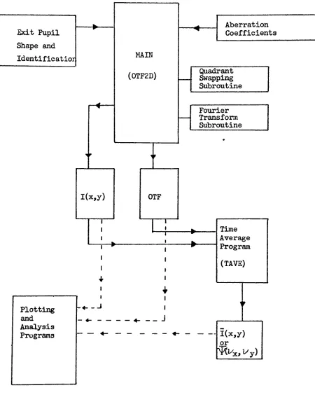
A system called

OTFBAR,

was designed

(Figure

15)

which would

calculate point spread functions and _{transfer functions for any} given

set of pupil shapes and aberration coefficients. The _{time averaging}

routine is a separate program capable of _averaging either the point

spread or transfer function data. Each surface generated is identified

with a pupil shape _{number, the} aberration _{coefficients,} and the value of

the shutter function as it is written to a _file. One- _{and two-dimen}

sional _plotting routines and a Tektronix

a006-1

computer graphics

terminal provide an efficient method of _comparing and _{analyzing the}

surfaces _{qualitatively,} so that significant results and unusual

asymmetries can be identified _rapidly and investigated in more

detail.

Essential to the OTFBAR system is the efficient and flexible

FORTRAN program titled 0TF2D which appears in appendix _{A. Data to}

0TF2D consists of the three aberration coefficients nC?n, QCi _n, and

2a

Exit Pupil

Shape and

Identificatior MAIN

(0TF2D)

I(x,y)

OTF

Plotting

and

Analysis

Programs

i

I

I

+

i J

l

i

l

I

J

Aberration

Coefficients

Quadrant

Swapping

Subroutine

Fourier Transform Subroutine

Time

Average

Program

(TAVE)

Kx,y)

or

Figure 15.

[image:33.551.47.497.52.616.2]

using small

arrays,

in batch with the array sizes

increased,

or in

batch

with magnetic tape to process a large number of exit pupil shapes.

An outline of the algorithm used in 0TF2D is shown in figures 16

and

17.

The wave aberration function

W(kg

>k

)

is generated once in

step

3

for a given set of aberration coefficients and placed in a

file if needed for _processing subsequent shutter frames. The shutter

shape is entered at the

beginning

of the

loop

at point

$.

In steps

7

and

8

the pupil function

?(k&

,k

)

is formed and prepared for the

fast Fourier transform routine. Equations 26 through

29

are evaluated

in steps

6-1

6.

If required the spread _{function may} be written to a

file in step

12,

and the

OTF,

frame identification _number, the

aberration

coefficients,

and the value of the shutter function is

written to a file in step

17.

At point 18 the program is completed

and will exit or return _{to step} number 2 for a new shutter

frame.

In its present form 0TF2D requires 21 K words of core and .3

minutes of CPU time in order to process a single shutter shape defined

in a

33X33

element array. Single frames _may be processed on-line as

the core requirement is small. The Total CPU time for a set of

thirty-six shutter frames is on the order of ten _{minutes, placing}

very little demand on the Sigma Six system.

The array dimensions of _{0TF2D may be increased} without

difficulty

in order to process a

65X65

array.

The

core requirement is then

56K

with

1.3

minutes of CPU required to process one frame and

approximately

50

minutes for thirty-six

frames.

Processing

on-line with the

larger

arrays is not possible due to a 32K on-line

limit,

and _{processing for}

26

START

'Enter

the

/number

of

frames: INUM

Enter the

aberration

coefficients

Generate the circular pupil

function containing

W(kg

,k

)

Enter frame ID

'number

and the

fshutter

shape

A(kg

,k

)

Store

rW(k4,k^)

inj

fa

file if

INUM>1

Calculate the value of the

shutter function S(t2

)

6.

Multiply

Wdc-j

,k^

)

by

A(k^

,k^7)

and obtain the pupil function

Call subroutine

SWAPQD(+1)

8*

to arrange the quadrants

containing

P(kg

.k,.

)

for the FFT

<b

Figure

16.

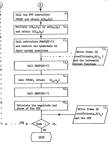
[image:35.551.92.498.44.684.2]

9

i

t

t

r

L

Call the FFT subroutine

F0UR2 and obtain a(kxky)

Multiply

a(kx,ky)

by

a*(kx,ky) 1G

and obtain

I(kx,ky)

Call subroutine

SWAPQD(-1)

--and restore the quadrants in

their normal positions

Call

SWAPQD(+1)

13.

ia.

Call

F0UR2,

obtain

(nx>-0

-w.

Call

SWAPQD(-1)

Calculate the magnitude and phase of the OTF

1BT

YES

JNUM O"

18.

NO

STOP

12.

fWrite

frame ID

/coefficients, S(t^

)

the

intensity

^spread

function

'Write frame ID

^

_coeff

icients,

S(

t.

)

(and

the OTF

Figure

17.

[image:36.551.74.515.36.628.2]

28

Provided sufficient accuracy is obtained, 0TF2D written to transform

a pupil function defined

by

a

33X33,

in a

6a

X

6a

working array

satisfies the OTFBAR system requirements and at a low cost in computer

resources

The OTF and spread function data is time averaged with the

program titled TAVE

(appendix

B). The values of each spread function

or _OTF surface are scaled

by

the shutter function S(t.

)

obtained

in 0TF2D. The weighted sequence of two-dimensional functions are

suimned and normalized to 1.0 at zero spatial

frequency

or at x=y0.0

in the image plane.

The

result is written to a file in a form

acceptable _{to the plotting} routines

COMPARE,

OTFPLOT,

AND PL0T3D

which appear in appendix E.

The program titled SHAPE

(Appendix

C)

was written to generate

input data for 0TF2D which would simulate a circular shutter with a

specific shutter function S(t). SHAPE can create one or more arrays

representing digitized circular exit pupils with varying

diameters.

The elements of the arrays are 1.0 for

100%

amplitude transmittance

for points within the shutter

boundary,

0.5

at points of

discontinuity

as required

by

the Fourier

transform,

and 0.0 for points outside the

shutter boundary. Each array is assigned a frame identification number

and is written to a file on magnetic disk or magnetic

tape.

The

data used to model the effect of a leaf-type shutter was

obtained from a high-speed film.

Thirty-six

16mm images of a

five-bladed Copal shutter _{in its closing} cycle were projected onto a

ao

cm

grid _containing an _array of

33X33

points. Each image was digitized

boundary

of the shutter

image.

It was _assumed, for simplicity, that

none of the _array points coincided with a

discontinuity

of the pupil

function.

The digital representation of each shutter image was recorded

with the program titled DIGIT

(appendix

D). DIGIT will accept the

column coordinates of elements with value 1.0 for each row, then

display

the entire image with row and column coordinates for a visual

check of the data entered. After any necessary corrections the data

for that image is written to a file in a form acceptable for _processing

with 0TF2D.

Approximately

seven hours total were required to digitize

the thirty-six 16mm images with this method.

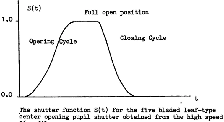
The opening sequence of the shutter was not digitized as the

shutter function shown in figure 18 would be assumed symmetrical

and with no

delay

in the full open position. The shutter _efficiency

of this model could be increased from

50% by including

a number of

full open circular shapes generated

by

program SHAPE.

Several transfer functions for various amounts of defocus and

spherical aberration were calculated for a single circular pupil

defined in a

33

X

33

array to establish the _accuracy of

0TF2D.

The

aberration-free time averaged OTF for the circular shutter model

was then calculated and compared to a second numerical solution to

establish the accuracy of the OTFBAR system.

Finally

time

independent

and time averaged transfer functions for various aberrarions were

calculated for both circular and leaf shutter models. The results are

30

i.o.

Full open position

Closing

Cycle

0.0

The shutter function

S(t)

for the five bladed leaf-type

center _opening pupil shutter obtained from the

high

speed

16mm film.

1.0

0.0

s(t)

A schematic representation of the discrete shutter function S(t.

)

created _{from the closing} cycle shown

above, and used to weight the time averaged OTF for the leaf-shutter model.

Figure

18.

[image:39.551.60.439.77.284.2]

IV. RESULTS

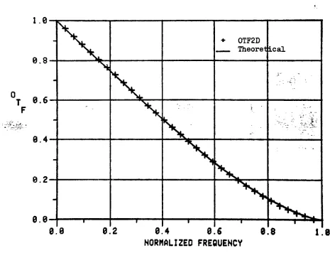
The _accuracy of the program 0TF2D for a

6a

point transform and

the case of a single circular exit pupil generated

by

the program

SHAPE is illustrated in figures

19

through 22. Because the

two-dimensional transfer function has rotational _symmetry about

the line 1/ a _V = _{0.0 for a circular exit}

pupil, any section in one

x _y

dimension

describes it completely.

1.0

0.8

6.2

0.4

e.e

NORMALIZED

FREQUENCY

0.8

1.8

Figure

19.

The OTF for a diffraction limited optical system as calculated

[image:40.551.46.511.255.611.2]

32

In figures one and two the 32 values returned

by

0TF2D for

0C20"oCao"oC60

s _{' ^} compared to the values given

by

the equation* :

OTF(y)

-A(y-Cosy

Sin

y)

y-

Cos"1(t-7i)

which describes the diffraction limited OTF exactly. Figure two

indicates an _accuracy of

-.005 OTF units for this particular set

of aberration coefficients.

(30)

X18

-2

9.4

8.2

Q

w

8.8

Eh

i

CO

9

-8.2

-8.4-

-0.6-+ -0.6-+ -0.6-+

'

^t'^v-0.0

0.2

++

0.4

+

+

+

0.6

.. -"; JrJ.f

0.8

1.0

Normalized Spatial

Frequency

Figure 20.

Absolute error in the diffraction limited OTF using the

theoretical results as reference.

Because the shape of the spread function changes with the

aberration _{coefficients, the} amount of error due to truncation in

image space changes also. In figures 16 and

17

the 0TF2D values

for one wave of defocus and ./fT waves of defocus are compared to

those published

by

Barakat and

Houston(21),

and Steel(22).

Only

a few of the numerical values in figures 16 and

17

can be compared

directly,

as the values in the literature are not computed at

normalized

frequency

increments of

1/32.

However,

"a comparison of

those points which do coincide indicate agreement within + _.005

3a

1.25

1.00

8.75-r

%

8.50-8.25

0.00

-0.25

iL

X

--*.

0.0

ma>o<

0.2

^>oo^oc:ooo

X Barakat

0 0TF2D

I

|

I

0.4

0.6

NORMALIZED

FREQUENCY

0.8

"r

1.8

Figure 21.

[image:43.551.25.480.232.573.2]

1.0

0.8

T

8.6

F

0.4

0.2

0.0

3l

x

*

0.0

0.2

a

x

a

FFT

Steel

*b

I

8.'4

0.6

NORMALIZED

FREQUENCY

0.8

1.8

Figure

22.

[image:44.551.33.465.238.599.2]

36

To test the entire OTFBAR system a sequence of 36 circular

exit pupils were generated

by

SHAPE which would simulate a circular

center _opening pupil shutter with a symmetrical shutter function

and a shutter _efficiency of

50

percent. The diffraction limited

time-averaged OTF values for this model are compared in figure

six to those given

by

the analytical function :

Y(U)

--T^

TTT'

y(u,t)-Cosy(u,t)

Siny(u,t)

dt

Where,

"X(u,t)

= _Cos-1 u/(2t/T)'

(3D

Figure

2a

indicates that the OTFBAR system values are con

sistently less than those given

by

equation 31 with a maximum

absolute difference of .005 OTF units.

X18

-2

0.0

0.2

0.4

0.6

NORMALIZED FREQUENCY

8.8

1.8

Figure 2a.

[image:46.551.41.464.228.579.2]

38

The effects of a leaf-type center _opening pupil shutter on the

two-dimensional

time-averaged OTF as predicted

by

the OTFBAR system are

illustrated

in figures

25

through

30.

The diffraction limited OTF

for a circular exit pupil shown in figure

25

may be compared to

figure 21_, the diffraction limited transfer function produced at

one instant in time

by

the _partly open leaf shutter. The

time-averaged sequence of 36 shutter frames produced the OTF shown in

figure

27,

a

smoothed,

symmetrical surface which does not exhibit

the vane-like structure shown in figure 26. Figures 26-30 show

the effects of

introducing

one wave of defocus. As would be pre

dicted

by

an _elementary geometrical model the time-averaged transfer

function surface retains vane-like structure when the aberrations

are large

(

> _{1 wave). In all cases investigated the magnitude}

of this irregular structure is on the order of +

.005 OTF units.

Consequently

a one-dimensional OTF curve _{corresponding} to a

section _{along the} 1/ axis is a _satisfactory representation of

OPTICAL

TRANSFER FUNCTION

FRAME

ID*

23

0C20-.088

[image:48.551.25.460.207.605.2]

0C40'

888

0C60- .008

SCTW.800

Figure 25.

The two-dimensional diffraction limited OTF for a circular exit

ao

OPTICAL

TRANSFER

FUNCTION

FRAME

ID

7

0C20* .008 0C40'

000

0C60-

888

S<T> .315

Figure

26.

[image:49.551.38.488.186.632.2]

OPTICAL

TRANSFER FUNCTION

FRAME

10=999

0C20

.800 0C40-

008

0C60- .000 8<T) .890

Figure 27.

The time-averaged two-dimensional diffraction limited OTF for

[image:50.551.20.503.208.607.2]

a2

OPTICAL

TRANSFER

FUNCTION

FRAME

IO*

25

0C20

1.088

0C40 .088 0C6Q" .888

S<T)1.809

Figure 28.

The two-dimensional OTF for a circular exit pupil and one wave

[image:51.551.34.480.181.569.2]

OPTICAL

TRANSFER FUNCTION

FRAME

10=

7

0C20

1.000

0C40*

000

0C60-

008

S(T) .315

Figure

29.

The two-dimensional OTF for one frame of the leaf shutter

[image:52.551.33.466.199.566.2]

aa

OPTICAL

TRANSFER

FUNCTION

FRAME

10=999

0C20*

1.000

0C40= .000 0C60 .000 8<T>* .099

Figure

30.

The two-dimensional time-averaged OTF for the leaf shutter

[image:53.551.15.465.203.566.2]

The effects of shutter motion on the time-averaged OTF as pre

dicted

by

the circular and leaf shutter models for various values of

the aberration coefficients are shown in figures 31-ao. As indicated

in figures

35

and 36 the difference between the values predicted

by

the two models varies with

frequency

but lies within + .06 OTF units

when _{the only} aberration present is defocus. Both of the models

indicate an increase of ten percent in the low

frequency

region of the

OTF for the largest

(one

wave) amount of defocus when compared to

a system with the shutter removed. The effect of _varying the

defocus coefficient

QC?n with and without a leaf type shutter in

the optical system is indicated

by

figure

37

at a normalized

frequency

of .25 The value of the transfer function is reduced in the

presence of the shutter as much as ten percent for small values of

0^20

(0-0-0.3)

and then increased to as much as ten percent for the

larger values of

a6

1.0

o

No Shutter

Circular

Leaf Shutter

Shxtter

I

|

l

1

1

|

I

e'e

0.2

0.4

0.6

0

NORMALIZED FREQUENCY

[image:55.551.29.476.242.591.2]

8

1.8

Figure 31 .

8.4

8.6

NORMALIZED

FREQUENCY

1.8

Figure

32.

[image:56.551.35.464.206.612.2]

as

i

1

i

|

r

8.4

8.6

NORMALIZED FREQUENCY

Figure 33.

[image:57.551.24.468.243.569.2]

1.25

1.80

0.75

0.50

0.25

0.00

-0.25

0.0

0.2

T

J

1

j

I

0.4

0.6

0.8

1.0

NORMALIZED FREQUENCY

Figure

3a.

[image:58.551.36.478.236.563.2]

50

9.84

0.02

Ert

O

<

-0.02

-9.04

0.00-O

0.0

0.2

0.4

0.6

NORMALIZED FREQUENCY

8.8

1.8

Figure 35.

The difference between the values predicted

by

the leaf [image:59.551.37.465.245.569.2]

E-i

O

<

8.88

0.86

0

04

0.02

0.00H

-0.82|

1

1

1

j

1 1 1

j

r

0.0

0.2

0.4

0.6

0.8

1.8

NORMALIZED FREQUENCY

Figare-36.

The difference between the values predicted

by

the leaf

52

0.8

0.6

T

0.4

F

0.2

-v

0.0

-0.2

No Shutter

Leaf Shutte:

X X

...A.

. :>m

-. z-<

'mm-'"-yzz?^

-'-'.

"

^

^

1 .. ,,

t ....

0.0

0.2

0.4

0.6

0C20

0.8

1.8

Figure 37.

The time averaged OTF at

V/v

[image:61.551.25.469.248.608.2]

Figure 38 indicates a much greater effect on the time averaged

OTF when _{the only} aberration present is one wave of third order

spherical. The OTF is increased as much as .15 OTF units according

to the leaf shutter model and.20 OTF units according to the circular

shutter model. The increased difference between values predicted

by

the two models for spherical aberration is shown in figure 39. A

maximum difference of .09 OTF units occurs at the normalized spatial

frequency

.125

If in

designing

or _constructing an optical system the coefficients

for third and fifth order spherical aberration are such

that,

0Cao/oC60

a _-3/2

the wave front is shaped so that the marginal rays converge at the

paraxial focus position as shown in figure

ao,

and the system is said

to be

fully

corrected.

Following

the notation in

0*Neill(23)

the

aberration polynominal _may be written _as,

A(p)

_0C60 (p6 - 3/2p^ +

3/a^.p2)

(32)

where/1, in terms of the residual maximum longitudinal spherical

aberration

&

L and the displacement of the _receiving plane from

HiL&

the paraxial focus position df is given

by,

max

Ad indicated in figure

ai

the two shutter models agree

within + _.005 OTF units when

qC^q

=

a.O

_{in equation}

(32)

and the

system is focused at the _normally optimum position given

by

fj. = _0.8

The effects of varying the focus parameterfj,on the time averaged

5a

1.25

1.00

0.75

0.50

0.25

0.00

-9.25 1

j

r

0.0

0.2

0.4

0.6

8.8

NORMALIZED FREQUENCY

Figure 38.

The time-averaged OTF for one wave of third order spherical

[image:63.551.39.465.234.570.2]

8.19

0.0

0.2

0.4

0.6

NORMALIZED FREQUENCY

8.8

1.8

Figure 39.

The difference between the values predicted

by

the leaf

shutter and circular shutter models for one wave of third order

[image:64.551.35.468.241.566.2]

56

I

Receiving

plane

Paraxial focus

Optical axis

Figure

ao.

The _{relationship between the wave-front,}

Sl

, and

Sf.

[image:65.551.53.506.69.324.2]

1.8

T

1

1

1

1

0.0

0.2

0.4

0.6

0.8

NORMALIZED

FREQUENCY

Figure

ai

.

The time averaged OTF at the optimum focus position

(JLl^.S)

for an optical system with both third and fifth order spherical

[image:66.551.35.464.239.627.2]

58

Figures

a2(a).

-

a2(i).

The effect of

defocusing

a fully-corrected optical system

on the time-averaged OTF for the leaf shutter

(+)

and on the

1.25

1.08

0

75

0.50

0.25

0.00

-0.25

0.4

0.6

NORMALIZED

FREQUENCY

60

0

1.25

1.80

0.75

9

50

8.25

0.00

-0.25

0.0

^

. . .

r

0.4

0.6

NORMALIZED

FREQUENCY

8.8

1.8

0

1.25

1.00

0.75

0.50

8.25

0.00

0.25

0.0

0.2

t

1

1

j

r

0.4

0.6

NORMALIZED

FREQUENCY

8.8

1.0

62

0

1.25

1.00

8.75

0.50

0.25

0.00

-0.25

M- = _0.6

-Yf

+ .

-

<^

",'-:K+-4-+-*

^4^^,

1 1 1 1

0.0

0.4

0.6

NORMALIZED FREQUENCY

0.8

1.8

1

0

0.0

0.2

0.4

0.6

8.8

NORMALIZED FREQUENCY

1.0

6a

1.25

1.00

0.75

8.50

0.25

0.08

-0.25

"*

/< = i-o

-r "" "

r i t

0.0

0.4

0.6

NORMALIZED FREQUENCY

8.8

1.0

0

1.25

1.80

0

75

0.50

0.25

0.00

-8.25 > p

0.4

0.6

NORMALIZED FREQUENCY

1.0

66

0

1.25

1.80

8.75

0.50

9.25

8.00

0.25

y***^;*-*!

lllllll

|if.|

|

/t = iy

,

|

1

1

r

|

1 i

0.0

0.2

0.4

0.6

0.8

1.8

NORMALIZED FREQUENCY

0

1.25

1

00--0.75

0.50

0.25

0.00

-8.25

0.0

ihd-h*

0.2

M-M

t

H

^

= _lr6

r

0.4

o.'e

NORMALIZED FREQUENCY

0.8

1.8

68

V. SUMMARI

Comparison of the values generated

by

the program 0TF2D and the

OTFBAR

system with literature and theoretical values indicate an

accuracy of + _.005 OTF units with the pupil defined in a

33

X

33

array and transformed with the FFT in a

6a

X

6a

working array. The

rapid oscillations of magnitude .001 OTF units illustrated in figures

20 and

2a

may be attributed to

leakage,

the picket, fence effect, and

machine round off.

Collectively

the errors could be reduced to give

an over all _accuracy of

+_

.001 OTF units

by

increasing

the working

array size to 128 X 128 elements.

However,

an overall _accuracy of

+_

.005

is _{judged satisfactory for the} purpose of

identifying

the effects of

shutter motion on the time averaged OTF.

The two-dimensional graphs created with the program PL0T3D

clearly indicate the dependence of the transfer function on pupil

shape. Figures 26 and

29

indicate the contribution of an individual

shutter frame while figure 30 and the numerical data indicate that the

time-averaged OTF is smooth enough to be characterized

by

a single

section _along one dimension. Attempts to plot _{corresponding} spread

functions in three dimensions indicated that a _{larger array} and a

plotting instrument with high resolution would be required to delineate

the small minima or side lobes. The three-dimensional plots proved

valuable in presenting a _complete, qualitative representation of the

two-dimensional transfer function.

The circular and leaf shutter models were in close agreement.

OTF than the leaf shutter model in the low

frequency

region.

This might be attributed to the difference in shutter functions

as

illustrated

in figure

a3

. Frames 1-1

3

used in _generating the

circular model transfer

functions,

were weighted from

2%

to

8%

more than the frames for the leaf shutter model.

Similarly

frames 19-32 for the leaf model were weighted

2%

to

5%

more than

the circular shutter model and the OTF predicted

by

the leaf shutter

model is higher than the OTF for the circular _{modql in} the high

frequency

range. This suggests that agreement between the two

models would improve if the shutter functions were identical.

In that case the effects predicted

by

the circular model would

be _{satisfactory in predicting the} effect of a semi-circular

center _opening pupil shutter on image quality.

In _obtaining the leaf shutter data it was assumed for con

venience that the

boundary

of the exit pupil did not lie on a

single sampling point. The assumption is valid in view of the

accuracy of the subjective method used in

digitizing

the exit

pupil. To eliminate the subjective analysis and in order to

process a large number of frames the OTFBAR system could be

interfaced with a computer controlled image _{scanning device.}

In addition to

identifying boundary

points an estimated reduction

in the amount of time required to digitize the exit _pupil, from

seven hours of operator time to one hour of machine

time,

would

be expected.

If we assume that detail corresponding to a given spatial

the effect of shutter motion on resolution in the exposure image

may be

determined

from figures

a2(a)~a2(I)

for the case of a

well-corrected optical system.

Figure

a2(e)

indicates a re

duction

in resolution due to the presence of the shutter when

the receiving plane is located at the position of best focus

(

/1=

.8).

Shifting

the _receiving plane toward the paraxial

focus

(

/_L =

.6) produces a very slight increase in resolution as

shown in

a2(d),

while further amounts of _{defocus corresponding}

to values of (J, less than .6 or greater than .8 does not produce

a recognizable effect on resolution.

An indication of the depth of focus in an optical system

is given

by

the amount of defocus required to reduce the value

of the OTF to 0.10 at a given spatial frequency.

Hence,

the

effect of shutter motion on depth of focus _{may be} obtained

from figures

37

and

a

a

which indicate the value of the time

averaged OTF as a function of the aberration coefficient

0C20,

and LLat

VAy

=0.25. In the presence of shutter motion

c

figure

37

indicates an increase in depth of focus* on the order

of + .2\n when the system is diffraction limited and focused

at infinity. This is a negligible increase in depth of focus in view of the Rayleigh quarter wave rule which indicates that

a difference in focus position of + wovld require a

considerable amount of effort to detect in terms of performance.

Applying

the same criteria to figure

a3

indicates that there is

also a negligible increase in depth of focus when the system is

72

Figure

aa..

The effect of

defocusing

a

fully

corrected optical system on the OTF at

Wt/C

[image:81.551.42.471.238.585.2]

The OTFBAR system has been used to investigate the effects

of a center

opening

pupil shutter on the time-averaged optical

transfer

function in the presence of defocus and spherical

aberration. The over-all effect of the shutter is to degrade

the OTF in the presence of small aberrations

(A

_=0.5), and

in well-corrected optical _systems, while _creating a slight

inqprovement

for larger

(A

1

.0) aberrations. In view of the

fact that the effects are small and will decrease with

increasing

shutter _{efficiency it is unlikely} that

they

are significant in

routine pictorial photography.

*The longitudinal displacement of _{the receiving} plane is given

by

L =

2qC2qR

/a

where R is the radius of the reference sphere and a is the diameter

7a

REFERENCES

1 . M. E.

Bechtel,

Cornell Aeronautical

Laboratory,

Rept. No.

VF-1260-P2,

Contract No.

AF33(6l6)-8870,

1959.

2. R. V.

Shack,

"The Influence of Image Motion and Shutter

Operation on the Photographic Transfer Function," _Applied Optics

(Oct.

196a),

Vol.

3,

No.

10,

pp. 117-1181.

"

3. J.W.

Cooley

and _{J. W.}

Tukey,

"An Algorithm for the Machine

Calculation of Complex Fourier Series," _Mathematics

of

Computation

(1965)

Vol.

19,

No.

90,

pp. 297-301.

a.

S. H.

Lerman,

"Application of the Fast Fourier Transform

to the Calculation of the Optical Transfer

Function,

"

SPIE MTF Seminar

Proceedings,

Rochester,

New

York,

(1968),

pp. 51-70..

5.

W. A. Minnick and J. D.

Rancourt,

"Transfer Function

Techniques for Real Optical Systems," _{SPIE MTF Seminar}

Proceedings,

Rochester,

New

York,

(196b),

pp.

87-103.

6.

R. C.

Baum,

Optical Transfer Function Calculation

by

the

Cooley

-Tukey Algorithm,

M. S.

Thesis,