The Optimisation of Bayesian Classifier in Predictive Spatial Modelling for Secondary Mineral Deposits

Procedia Computer Science 61 ( 2015 ) 478 – 485

1877-0509 © 2015 The Authors. Published by Elsevier B.V. This is an open access article under the CC BY-NC-ND license (http://creativecommons.org/licenses/by-nc-nd/4.0/).

Peer-review under responsibility of scientific committee of Missouri University of Science and Technology doi: 10.1016/j.procs.2015.09.194

ScienceDirect

Complex Adaptive Systems, Publication 5

Cihan H. Dagli, Editor in Chief

Conference Organized by Missouri University of Science and Technology

2015-San Jose, CA

The Optimisation of Bayesian Classifier in Predictive Spatial

Modelling for Secondary Mineral Deposits

Adamu M Ibrahim, Brandon Bennett, Fatima Isiaka *

Department of Computing, Sheffield Hallam University, United Kingdom

Abstract

This paper discusses the general concept of Bayesian Network classifier and the optimisation of a predictive spatial model using Naive Bayes (NB) on secondary mineral deposit data. A different NB modelling approaches to mineral distribution data was used to predict the occurrence of a particular mineral deposit in a given area, which include; predictive attributes sub-selection, normalised attributes selection, NB dependent attributes and the strictness to NB model assumptions of attributes independence selection. The performance of the model was determined by selecting a model with the best predictive accuracy. The NB classifier that violates assumptions of attributes independence was used to compare with other forms of NB. The aim is to improve the general performance of the model through the best selection of predictive attribute data. The paper elaborates the workings of a Bayesian Network learning model, the concept of NB and its application to predicting mineral deposit potentials. The result of the optimised NB model based on predictive accuracies and the Receivr Operating Characteristics (ROC) value is also determined.

© 2015 The Authors. Published by Elsevier B.V.

Peer-review under responsibility of scientific committee of Missouri University of Science and Technology.

.Keywords: Bayesian Network, Naive Bayes, Direct Acyclic Graph (DAG), Predictive Attributes, Cassiterite, ROC.

1. Introduction

Bayesian Networks (BN) also referred to as belief network is a probabilistic graphical model. Knowledge about vagueness domains are represented in a structural graph called the directed acyclic graph (DAG) [1]. Each graphical node is a representation of knowledge about an uncertain domain or a random variable, while the edges between two node represent probabilistic dependencies. The conditional independence described by graphs can be estimated using some known empirical methods. BN is a mixture of study probability, computer science, statistics and graphs [1]. DAG is commonly used by statisticians, machine learning experts or within Artificial Intelligence (AI) societies, it also enables the representation and computation of the joint probability distribution over a set of variables [1][17]. Two segments define the DAG structure; the nodes (vertices) and the directed edges also referred to as arcs. While

* Corresponding author. Tel.: +447841421372 E-mail address: [email protected]

© 2015 The Authors. Published by Elsevier B.V. This is an open access article under the CC BY-NC-ND license (http://creativecommons.org/licenses/by-nc-nd/4.0/).

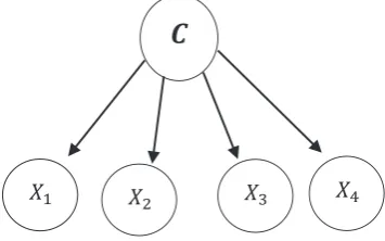
the nodes represent random variables and are labelled by the variable name, the edges represent the direct dependence among variables, using a drawn arrow between cyclic nodes as shown in Figure 1 [1].

The Figure I show direct dependence of value taken from ݔ௝ onݔ௜ or rather ݔ௜ has influence onݔ௝. Here, the ݔ௜node

was considered the parent and ݔ௝ the offspring to ݔ௜ [1]. The structure of the DAG ensures that no node can be its

ancestor or descendant, and this condition is vital for the factorization of the joint probability of sets of nodes. The reasoning process in BN transferred information from any direction and the causal effects are determined by the direction of the arrows [1] [18]. A more formal definition of Bayesian Network is represented by the pair [6];

ܤ ൌ ۦܩȁߠۧ

Where;ܩis the DAG, and ߠ represents the set of parameters of the network.

The structure as shown in Figure 1 representing the qualitative and quantitative parameters will need to be determined by probability values. The parameter is in tandem with the Markovian property where parent’s node indicates the

conditional probability distribution. The conditional independence statement which implies that each attribute (variable) is independent of any children in the graph given the state of its parent. Situation in which certain conditions are used in a joint probability distribution that minimises a number of efficient ways to compute the posterior probabilities. In a discrete random variable, a constructed table of local conditional probability was used to calculate the joint probability of the variables [1].

2. Bayesian Network Learning

Practically, BN settings are mostly unfamiliar as learning settings are learned from datasets called BN learning problems. The learning difficulties are stated as having a training data and a prior information (e.g., expert knowledge and causal relationship). The BN assessed the graph network arrangement and parameters of the joint probability distribution in the BN as indicated in Figure 2. Both BN graphical structures and parameters learning are of major concern in learning BN [3]. However, there are two ways of viewing a BN as an approach to learning; first is learning the variable arrangement that includes the joint distribution of the variables that best fit the data and leads to scoring--based learning algorithms. The network arrangement seeks to maximise the Bayesian or entropy scoring function [3]. The second is where the BN arrangement that includes the conditional independence relationship among the nodes (attributes) represented in the DAG nodes according to the concept of d-separation [17]. Learning the structure arrangements involves identifying the conditional independence relationships among the attributes. Some statistical test such as chi-square test, the correlation coefficient (covariance) among the attributes and the mutual information test were used to determine the conditional independent relationships among attribute nodes. The conditional independent relationships found in these attributes was used as constraints for designing a BN. The BN algorithm is also known as the constrained-based algorithms or CI-based algorithms [2, 19].

2.1 General Bayesian Network (GBN)

GBN deals with classification attributes cyclic nodes as regular nodes. It takes training and feature sets (along with nodes ordering) as input, determines the Markov blankets of classification node, delete all the nodes that are outside the Markov blanket, learn the parameters and returned the GBN as shown in Figure 2. The Bayesian Network considers the estimation of parameters and the directed acyclic graph from the training data using the score-based or dependency-based approach for posterior and prior probability values. The trained data may avoid the cause dimensionality problem by adopting n-1 fold since it is not possible to find an equal number of sets for the different data class. The idea of BN is concept-based from inception, but the advancement of AI led to the development of intelligent Bayesian called Naive Bayes (NB) capable of inductive learning and generalization [2,3,7,20]. It is also very tractable to statistical computation because the conditional probabilities are a measure of parameters of the inter-variable dependencies.

ݔ_݅ ݔ݆

3. Naive Bayes (NB) Network

Naive Bayes is a simple structure algorithm that has its parent node as its class and no further links is required in the NB structure [4]. It has an advantage over other classifiers because; it is easy to construct with a given priori as the structure of NB so that no structure learning procedure is required. The process of classification using NB is very efficient with both advantages assuming all features are independent of each other. The NB has performed better than so many classifiers in so many datasets, especially where the attribute’s datasets are less correlated (i.e., independent of features) [11]. Although BN is very effective for knowledge representation and inference under uncertainty, the BN was not regarded as a classifier until the discovery of the NB [17]. An ordinary constructed NB as indicated in Figure 3 adopts independence attributes, have shown greater performance than most classifiers [11]. According to Friedman et al.; "other forms of NB structure include Tree Augmented Naive Bayes (TAN), a situation where the algorithm first learns a tree structure over variable nodes X over class C i.e., ࢄȀሼ࡯ሽusing the mutual information test condition on C. [6].

Another form of NB is the BN Augmented Naive-Bayes (BAN); this is similar to TAN but extended the attribute that produced a random graph instead of tree structures [6].

4. The Proposed Improved Naive-Bayes Model

Optimising the algorithm may vary depending on the task the model intends to accomplish. In this classification modelling, the trade-off is between predictive accuracy, task execution speed, the simplicity of the algorithm and model generalisation. The purpose is to critically evaluate the NB modelling capability with a view to improve its predictive accuracy, reduce complexity of the model (i.e. easy to manage) by having less attribute’s data and reduce task execution time. This paper attempts to improve the performance of NB classifier. This attempt was based on feature subset selection and a relaxing independence assumption of the algorithm. Another approach was adapted to the feature selection and model assumption principle to optimise the NB model performance and conduct the best approach to model selection. The optimisation procedures employed includes:

x Feature subsets selection: Forward feature selection was used to obtain a good subset of attributes and construct the NB classifier with the selective attribute []. The data feature selection used the best-first search procedure based on attribute accuracy estimates to find sets of final attributes to include in the classifier [10,11]. The algorithm will select attributes with the least of error during model fitting.

x Attributes independence assumption: The NB assumption of independence allows the selection of attributes that are not strongly correlated, this can be achieved by determining the general covariance or correlation among the predictive attributes. The coefficient of all the attributes was presented as a correlation heat map as indicated in Figures 7 drawn to visualised correlation among attributes dataset. Only the uncorrelated attributes were selected, which satisfy the independently identical data assumption that allows independently, and less correlated attributes to build the model [14,12,13]. However, the assumption of attributes independence are often violated in a typical NB classification this is because, it is very difficult to achieve such in real life.

x Model simplification and task execution time: A simple algorithm is very easy to manage. The simplification could be in terms of the number of predictive attributes used in the model design. The attribute’s subsets are

ܺ_{ଵ ܺଶ} ܺଷ ܺସ

࡯

selected based on their importance to the prediction in determining the predictive accuracy of the model. Fewer attributes subsets selected may maintain the predictive accuracy or even outperformed the model built with a larger number of predictive attributes. In this case, the model becomes simpler with fewer attributes occupying less. The classification modelling has been known to accommodate very large datasets and this in turn takes time to execute in a computer program. In reality, the time taken task by a computer to execute a task depends on the volume of task or amount of data to be processed, which may be termed to be linear. Therefore, a reduction in the sets of the attribute without losing predictive accuracy or violating any model assumption or even making the model complex will certainly reduce the task execution time. The task execution time is very important for quick decision making as well as model implementation in s model deployment situation (embedded system).

5. Application of Naive Bayes to Mineral Potential Mapping

The application of NB algorithm to mineral potential mapping of mineral deposits, considers the composition of natural attributes describing the knowledge domain of the area as captured in the DAG represented in Figure 5. NB classifier is the simplest Bayesian Classifier used for mineral potential prediction [4, 11]. Even though the NB assumes total independence of predictive attributes, a very rare phenomenon in a real life situation, the NB still performs well when violated in several experiments. The performance of the NB models is further improved by relaxing some of the strict assumptions [16, 5, 6]. Six nodes simple Bayesian Network in Figure 5 represents the DAG consisting of directed edgesshowing conditional dependencies based on qualitative knowledge of the domain, i.e., from expert opinion on the formation of mineral deposit. The DAG suggests that topological and spatial configuration of nodes which shows causal relationships among attributes. The NB considers all the predictive attributes as independent of each other with the parents represented as the class as seen in Figure 5.

6. Data Selection and Attributes Extraction

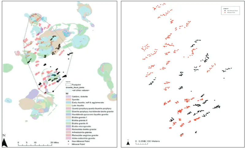
Data sets obtained from the field survey of an existing mining site representing an area where mineral deposits of a particular type have been found at the same time where the particular mineral have not been found. The surveyed mining sites contain a total number of 749 mining points, out of which about 463 have cassiterite mineral presence while 286 have no presence of cassiterite mineral. The survey was done in the Plateau Younger Granite Region of Nigeria (PYGR) with an area size of approximately 16,650 km2_{. In this area, several past and current mining sites}

were visited, and their accurate position measured (latitude, longitude and elevation). The survey team divides the mining district into eight discovered mining regions to ease the survey of mining sites within the study region. Each of this region contains lots of mining site. The team visited all past and current mining sites during the fieldwork and captured the relevant geological and geophysical data for all the observed mining points. The mineral points were selected according to the density of mineral occurrence such that places with high density are given fewer points and vice versa. Attributes such as the elevation of each point above sea level measured in meters and map of PYGR consisting of 204 digitised rock layers as polygons are the natural predictive attributes of the mineral deposit points. Other spatial and statistical attributes or parameters added to the datasets made a total of 21 predictive attributes. Binary classes of 0 and 1 were assigned to indicate absence and presence of mineral (in this case cassiterite) respectively.

The NB algorithm uses the domain data for training and developing a set of rules that will replicate the mapping between the features and class or between parent and dependants. NB algorithm do not require the study of the structural procedure, the applied structure for mineral potential mapping of the PYGR is as shown in Figure 5. The predictive attributes representing the knowledge domain of the PYGR mineral data potential distribution that includes:

15 G ranite and Non-G ranite R ock represented as R T ypes, C losest G ranite R ocks P erimeter size represented as R T ypes, 15 S patial attributes of distance from an observed mining point to the nearest 15 rock units represented as – S A, shortest nearest distance among the observed mining point to the nearest 15 rock units represented as – NND to R ock, L atitude represented as – L at, L ongitude represented as –

A total number of 21 features were extracted from the research area represented in Figure 4 to form the predictive attributes used for this experiment. Among the 21 attributes, all but except two are completely spatial attributes. The two non-spatial attributes are the rock type (size) and the probability weight of the closest rock to the point. However, attributes such as Latitude and Longitude and UTMs are not included in the final modelling selection or experiment because they represent spurious predictors that may mislead the predictor since attributes such as position on the earth surface are not transferable.

7. NB Optimisation and Result Presentation

The optimisation of the NB algorithm involves the evaluation of the model performance results using the standard method of Machine Learning Design Architecture [8] [9]. The model performance score is required to select the best model that fits the data and the performance is often data dependent. Therefore, the fitting patterns can provide the foundation in search for optimality [15]. Evaluating the predictive model’s performance is a process where results of

a model’s predictive accuracy produced is subjected to some quality test and making some few adjustments to improve

(optimise) its performance by producing improved predictive performance accuracy. The level of predictive accuracies obtained in the predictive model is data dependent as well as algorithm dependent. Hence, model optimisation starts from the level of data pre-processing by selecting the best predictive attribute and adjusting (relaxing or enforcing) some algorithm assumptions.

7.1 Attribute Independent Assumptions

The NB classifier was implemented by relaxing the basic assumption associated with the NB algorithm. In ordinary NB, the strict assumption rules are often violated [16][5][6]. By selecting all of the attributes describing the domain and excluding the latitude and longitude and Utmx and Utmy. The latitude and longitude were isolated from the final attribute selection to prevent error due to clustering and select only attributes that are transferable i.e., model attribute generalisation.

7.2. Selection of Predictive Attributes Important Subset

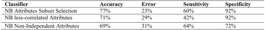
The most important attributes subset selection has reduces twenty-one (21) predictive attributes used initially for building a model down to four (4). Selection indicates that only four attributes are most important to predicting mineral occurrence with less error in modelling mineral occurrence using NB classifier. Indication of the slight improvement in the model accuracy performance is noticed when using the four sub-selected attributes as seen in the result of model performance given in the Table I. The model was simplified by using the few (selected) attributes to achieve higher predictive accuracies. The four attributes selected for optimisation include; the size of the rock in terms of area denoted as attribute – AreaR, the spatial distances (ND Rock) between mineral points (observation) to the three nearest granite rocks R15, R6 and R3, represented as attributes DR15, DR6 and DR3 respectively.

7.3. Restrictiveness to Model Assumption

Another set of data exploration analysis was the test of data independence. Since the NB algorithm assumes data independence as shown in the Figure 3, where all attributes are children of one parent ``C '' representing the class. A correlation of the entire datasets was conducted using correlation heat map to determine attribute’s independent. The heat map diagram, as shown in Figure 7 determines the correlation coefficient values and plot of covariance among predictive attributes. The heat-map was visualised to select attributes that are less correlated to use in the learning algorithm. Although a correlation may not necessarily mean causation, it still implies the existence of a relationship among predictive attributes. Therefore, care must be taken when selecting highly correlated attribute data so that the assumption of attribute independence is not violated. The value of correlation coefficient indicates the level of covariation among the attributes and as such may compromise data independence when the effect is very high. The highly correlated attributes are identified and removed from the training and testing data of the model. The results are as indicated in the Table I.

Classifier Accuracy Error Sensitivity Specificity

NB Attributes Subset Selection 77% 23% 60% 92% NB less-correlated Attributes 71% 29% 42% 92% NB Non-Independent Attributes 69% 31% 64% 72%

Table ITable I. Model performance table for all the NB classification approach.formance t bl f l it di l h l lit

8. Results

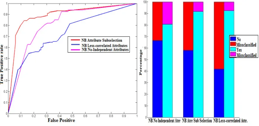
Based on the result of predictive model performance in the Table I, it is clear that the result of NB attributes subset selected design algorithm performed best with the lowest error rate and the highest predictive accuracy rate. An indication of overall model performance was presented by the area under the receiver operating characteristics (AU-ROC) curve plot shown in Figure 8; a trade-off between the true class and the false class (i.e., sensitivity against specificity). The performance of the NB attributes selected was further justified in Figures 9 which shows the percentage rate of model misclassification of the true and false classes. The least performing algorithm among the three NB algorithms used in the proposed optimised classifiers is the ordinary NB. The ordinary NB does violates the assumption of attribute’s independent and retains spatial autocorrelation among the predictive attribute’s data that causes the model to perform lower than the rest that have less correlated attributes in their models.

9. Conclusion

In this paper, the direct application of learning unrestricted Bayesian Networks for classification tasks using NB classifier has been analysed. We showed that, although the violation of the NB algorithm method presents strong, good predictive accuracy, it does not optimize the classifier of the learned networks. The results obtained in Figures 8, and 9 suggest a rather more simplified NB sub-selected attributes algorithm with fewer predictive attributes that

performs a similar task and improved predictive accuracy. The improvement in predictive accuracy score, task execution time, and simplicity with fewer attribute data shows some form of model optimisation of the NB modeling approach to mineral data prediction from the data perspective. The findings of this research also indicated that despite violating the NB model assumption of independence using ordinary NB algorithm approach, the model performs well having the highest sensitivity score, i.e., ability to predict not mineralised point better than the rest of the algorithms with a sensitivity score of 64%. The major contribution of this paper is the experimental evaluation of the NB classifier

and the attribute’s subset selection in the classifier. It is clear that the lack of conducting some exploratory data analysis many a time leads to the application of wrong algorithms to modelling distribution data. The situation made classification algorithms to perform poorly. Therefore, it is necessary to conduct the test of attribute independence when using NB classifier because of its strict assumptions to attribute data independence. Such concept will ensure the use of the right algorithm when faced with a classification problem. Still, both augmented NB and attribute subset selection NB techniques embody a good trade-off between the higher predictive accuracy and simplicity (non-complexity). The learning procedures are guaranteed to find optimal patterns, and, as the predictive performance results show, they performed well in practice with very fewer attributes. The optimisation process has shown an overall improvement in the NB attributes selection approach. Among the 3 NB approaches with highest Specificity score of 92% (i.e., ability to identify mineralised class) using only four (4) attributes from the initial twenty (21). The NB attributes selection approach also recorded to lowest misclassification rate as seen in Figure 9 and highest area under the ROC indicated in Figure 8. The overall predictive model performance was optimised using the NB attributes selection approach and is, therefore, proposed for implementation in an embedded working system.

References

1. Ben-Galand I, Ruggeri F, Faltin F, and Kenett R. Bayesian networks, encyclopedia of statistics in quality and reliability. Wiley & Sons, 2007. 2. Jie Cheng and Russell Greiner. Comparing bayesian network classifiers. In Proceedings of the Fifteenth conference on Uncertainty in artificial

intelligence, pages 101–108. Morgan Kaufmann Publishers Inc., 1999.

3. Gregory F Cooper and Edward Herskovits. A bayesian method for the induction of probabilistic networks from data. Machine learning, 9(4):309–347, 1992.

4. Richard O Duda, Peter E Hart, and David G Stork. Pattern classification and scene analysis 2nd ed. 1995

5. Nir Friedman. Inferring cellular networks using probabilistic graphical models. Science Signalling, 303(5659):799, 2004. 6. Nir Friedman, Dan Geiger, and Moises Goldszmidt. Bayesian network classifiers. Machine learning, 29(2):131–163, 1997.

7. Jeffrey A Hepinstall and Steven A Sader. Using bayesian statistics, thematic mapper satellite imagery, and breeding bird survey data to model bird species probability of occurrence in Maine. Photogrammetric Engineering and Remote Sensing, 63(10):1231–1236, 1997.

8. Adamu M. Ibrahim and Brandon Bennett. The assessment of machine learning model performance for predicting alluvial deposits distribution. Procedia Computer Science, 36(0):637 – 642, 2014. Complex Adaptive Systems Philadelphia, fPAg November 3-5, 2014.

9. Adamu M. Ibrahim and Brandon Bennett. Point-based model for predicting mineral deposit using GIS and machine learning. In Proceedings

of the 2014 First International Conference on Systems Informatics, Modelling and Simulation, SIMS ’14, pages 83–88, Washington, DC, USA, 2014. IEEE Computer Society.

10. Ron Kohavi and George H John. Wrappers for feature subset selection.Artificial intelligence, 97(1):273–324, 1997.

11. Pat Langley, Wayne Iba, and Kevin Thompson. An analysis of Bayesian classifiers. In Proceedings of the National Conference on Artificial Intelligence, pages 223–223. JOHN WILEY & SONS LTD, 1992.

12. Pierre Legendre. Spatial autocorrelation: trouble or new paradigm? Ecology, 74(6):1659–1673, 1993.

13. Pierre Legendre, Mark RT Dale, Marie-Jos´ee Fortin, Jessica Gurevitch, Michael Hohn, and Donald Myers. The consequences of spatial structure for the design and analysis of ecological field surveys. Ecography, 25(5):601–615, 2002.

14. Jack J Lennon. Red-shifts and red herrings in geographical ecology. Ecography, 23(1):101–113, 2000.

15. Mwitondi KS, Moustafa RE and Hadi AS. A data-driven method for selecting optimal models based on graphical visualisation of differences in sequentially fitted roc model parameters. Data Science Journal, 12(0):WDS247–WDS253, 2013.

16. Michael J Pazzani. Searching for dependencies in bayesian classifiers. LECTURE NOTES IN STATISTICS-NEW YORK-SPRINGER VERLAG-, pages 239–248, 1996.

17. Judea Pearl. Probabilistic reasoning in intelligent systems: networks of plausible inference. Morgan Kaufmann, 1988. 18. Judea Pearl. Bayesian networks. 2011.

19. Peter Spirtes, Clark Glymour, and Richard Scheines. Causation, prediction, and search, volume 81. MIT press, 2001.