Working Paper - Exploring changing social structures and health using the Health Survey for England: a technical note on the creation and analysis of a time-series dataset in SPSS

(1)

White Rose Research Online

[email protected]

Universities of Leeds, Sheffield and York

http://eprints.whiterose.ac.uk/

White Rose Research Online URL for this paper:

http://eprints.whiterose.ac.uk/77494/

Working Paper:

(2)

1

Exploring changing social structures and health using the Health Survey for England: a

technical note on the creation and analysis of a time-series dataset in SPSS

Abstract

This technical note will discuss the processes involved in creating a time-series dataset for the Health

Survey for England (HSE) from 1998 to 2011. This dataset has been used to explore the changing

structure and composition of England’s society over time, and then to consider what implications this

has for inequalities in health. The HSE, an annual nationwide household survey which is

geographically, socially and demographically representative of the England’s residential population

is an ideal data source for analyses such as this. Despite the richness of the HSE a lack of variable

consistency between survey years hampers analysis of change over time. To successfully explore

change, variables of interest must be either derived or recoded before a new, harmonised dataset can

be created for analysis. This report will outline the methods required to extract variables of interest

and then harmonise inconsistent variables. Some discussion will also be presented on the main

statistical methods used within the final analysis as this influences some of the choices made in data

preparation.

Introduction

This technical note will provide an account of the methods used to create and analyse a time-series

dataset drawn from the Health Survey for England (HSE). Similar to other technical notes reporting

on the creation of a time-series dataset using the HSE, an executive summary will be included which

summarises the steps used (see figure 1). Any prospective user of either the HSE or another similar

source who wishes to create a time-series dataset can then follow these generic steps without

reference to the specific details. Those interested in working with time-series datasets should refer to

other comparable work from Vanessa Higgins and Alan Marshall (2012) who also used the HSE to

create a time-series dataset to analyse trends in obesity. Although this report will provide a linear

account of the main steps taken to create the final dataset, the actual process itself is more iterative

whereby variables may be dropped or further amended to suit the needs of the statistical analysis.

For this research, the dataset created has been used to explore what implications the changing

structure and composition of England’s society has had for population health. Whilst a full discussion

of the analysis will not be presented here, the following section will briefly set out the background to

this research. This should give the reader sufficient information to understand the decisions made

regarding the chosen dataset, variables of interest and statistical methods. Theoretical justifications for

these choices will not, however, be discussed. Having set the context within which this dataset was

created, the HSE itself will be briefly introduced. More extensive reviews of the HSE can be found

(3)

2

This will be followed by the executive summary noted above. The remaining sections first discuss in

detail how each variable of interest has been harmonised before briefly discussing some of the

statistical tests used to analyse the data. Tables for each harmonised variable are included clearly

illustrating how the original variable categories have been manipulated to create the final harmonised

version. The final section acts as an illustrative example of the kind of the steps a researcher might

take to analyse trends over time using, in this instance, binary logistic regression. Within the report,

example lines of syntax are presented where required with the full syntax used included in Appendix

A.

Background: why explore change and what implications for health?

The structure and composition of England’s society is dynamic. Whilst England may arguably remain the most ‘class-ridden country under the sun’ this is not to suggest that this class structure has

remained static since Orwell’s damning account (Orwell, 1984: 29). The de-industrialisation of the

workforce which led to an increasing shift from manual to non-manual occupations has altered the

class structure of society. As the labour or class structure of society varies, so too do other

socioeconomic structural features. For example, England’s society may be increasingly educated yet

this is not necessarily equitable across population subgroups defined by anything from class to

geographic location (ONS, 2013). Structural changes to society are also accompanied by

compositional changes: England’s population is increasingly ethnically diverse (ONS, 2012) and also

ageing (Jowit, 2013). Any analysis of structural change should concurrently consider compositional

change as the two are inter-related. For example, an ageing population will inevitably influence the

distribution of the population by economic activity status. Exploring structural and/or compositional

change in society over time may provide insight into a whole range of sociological, economic and

political phenomena. Crucially for this analysis, however, it may also be revealing with respect to

changing inequalities in health.

Inequalities in health are widely observed and there is convincing evidence to suggest that, for some,

these gradients are widening (Norman et al., 2011; Shaw et al., 2004; Thomas et al., 2010). These

socioeconomic and spatial inequalities in health stem from the social and spatial gradients health

follows (Chandola, 2012). It is therefore likely that structural and compositional changes to England’s

society may influence health gradients. Furthermore, as inequalities in health are also found by

ethnicity (Nazroo, 2006), it is important to explore whether different ethnic groups have experienced

different structural changes which may affect health inequalities.

If we assume that societal change does indeed have implications for population health, it is then

important to select a dataset which is rich enough to concurrently explore structural, compositional

and health change in the population over time. Whilst a variety of potential sources exist, the research

(4)

3

The Data

Since 1991, the HSE, an annual household nationwide survey, has been collected with the intent of

providing public health professionals and academics with information about the health of the

population and to reveal trends in health-related behaviours. Each year, the survey focusses on

different population subgroups (such as the elderly) or specific morbidities (such as cardiovascular

disease) alongside a set of core questions covering socioeconomic, demographic and general health

variables. Stratified random sampling of individuals from a sample of postcode sectors each year

ensures that the survey sample is representative of the England’s population both in terms of their

socioeconomic composition and geographic distribution. The potential for analysing structural,

composition and health change is clear. However, despite the richness of this particular dataset, any

analysis concerned with change may be hampered by the potential inconsistency of the variables

between survey years. Consequently, before any analysis can be completed, selected variables must

(5)

4

1. Download Health Survey for England (HSE) datasets:

1998; 1999; 2000; 2001; 2002; 2003; 2004; 2005; 2006; 2007; 2008; 2009;

2010; 2011

2. Identify variables of interest relating to:

Health; demographics (e.g. age, gender, ethnicity); socioeconomic circumstances (e.g. social class, household tenure, education) [see

table 1 for full variable list]

NB: Each file downloaded contains two datasets, the household and the individual denoted by either ‘ah’ or ‘ai’ within the filename. All variables should be taken from the individual dataset. For 1999 and 2004, the ethnic boost years, three datasets are provided. As one of

the principle interests for this analysis was to explore ethnic inequalities in health, using a boost sample where minority ethnic groups were oversampled may skew the results. Consequently, the boost sample should not be used. 2000 and 2005 were also boost years but for older people and no separate datasets were provided.

These were therefore included within the analysis but necessary caution should be taken when interpreting results from these years.

3. Harmonising and recoding variables:

Variables which are either not consistent over time (either in the

variable name or variable categories), need manipulating to meet the needs of the statistical tests

used or where new variables are derived from existing ones should be

harmonised and recoded according to the syntax described below.

4. Extracting relevant variables into new datasets:

Variables should then be extracted, either in their existing state or as

newly harmonised or derived variables into a series of new datasets. Syntax described below.

5. Creating a time-series dataset and considerations:

Combine all new datasets into a single time-series. Determine whether survey weights should be used and check dataset

for any problems which may arise from variations in sample sizes, e.g. boost years.

6. Analysis:

Analyse the data using various statistical tests including binary logistic regression. To improve the statistical power of analysis

and smooth out random fluctuation, trends should can be explored across pooled rolling three-year averages of groups of

[image:5.842.31.777.71.478.2]

(6)

5

1. Downloading the data

All data can be accessed and downloaded from the Economic and Social Research Council’s (ESRC)

UK Data Service following registration with the site. Once registered, each survey year of interest can

be downloaded (in a variety of file formats including SPSS). Choice of study period depends on the

availability of variables of interest and the possibility of creating consistent variables for time-series

analysis. For this analysis, whilst the HSE began in 1991 the appropriate time-frame was from 1998 to

2011 owing to the availability or detail provided within key variables such as ethnicity.

2. Identify variables of interest

Variables of interest will differ according to the nature of the study. Furthermore, variables which

may initially be considered important may be subsequently dropped depending on the results of

statistical analysis. Thus, although the broad categories of interest for this analysis were health (the

dependent variables), demographics and socioeconomic status, some variables initially identified

within these themes were not included in the final analysis. For brevity, the following section will

only outline the re-coding, deriving or manipulation of variables which were actually used within the

analysis. However, as discussed in the introduction, once the analysis began further manipulation of

some of the variables was required. Thus, the variable format presented here may not match the

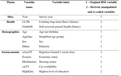
variable format of all the variables used within the final analysis.Table 1 lists these variables

according to their theme, and distinguishes between those which have been manipulated and those

which were used in their original format as supplied in the file.

When identifying variables of interest these should all be taken from the HSE file relating to

individuals (denoted by ‘ai’ in the file name), rather than households (denoted by ‘ah’). For 1999 and

2004, the surveys focussed on the health of minority ethnic groups (MEGs) and therefore provided a

third dataset where MEGs were oversampled. Ethnicity was a key variable for this work and much

may be gleaned from a standalone analysis of either the boost sample for 1999 or 2004. However,

including the oversampled data within the final time-series may bias the results. Consequently, these

boost files were discarded for 1999 and 2004, and the standard individual files used instead.

Although 2000 and 2005 were also boost years with people aged over 65 being oversampled separate

boost files were not provided. As it is assumed that all survey years available within the study

time-frame will be used these should be extracted as normal. The effect of these boosted samples on the

final results can be considered once the time-series dataset has been created and this is discussed

(7)

6

GET FILE='F:\Data\HSE\HSE

[image:7.595.65.537.100.398.2]

2011\UKDA-7260-spss\spss\spss14\hse2011ai.sav'.

Table 1: Variables in the dataset

Theme Variable

name

Variable label 1 – Original HSE variable

2 – Derived, manipulated

and re-coded variables

Misc. Year Survey year 2

Health LLTIb

Genhelfb

Limiting long-term illness (binary)

Self-assessed general health (binary)

2

Demographics Age

AgeGrps

Sex

Ethnic

Age last birthday

Simplified age groups

Sex

Ethnicity

1

2

1

2

Socioeconomic sclassTT

Econact

Hholdtenure

carTT

HighEduc

Registrar General’s social class

Economic status

Housing tenure

Car availability

Highest level of education

2

1

2

1

2

In SPSS, users are provided with the option of either working with dialogue boxes or using SPSS

syntax to complete tasks. Using SPSS syntax is a much more efficient way of working with large

datasets as syntax can be copied, pasted and re-used quickly without having to work through the

multiple options available in the dialogue boxes. For those unfamiliar with SPSS syntax, a number of

reference books are available (for example see Collier, 2010), as well as a wealth of freely available

information on forums and other internet sites. For clarity, all syntax presented in this document are

enclosed in a text box and, if the file paths and variable labels are correct, can be copied and pasted

for re-use.

Syntax can be used to open each survey year file. The ‘Get file’

command opens up any file on a computer directory so long as the

file path and file name are correct, this can be copied and pasted for

each survey year, amending the name as required.

3. Harmonising and recoding variables

Where required, manipulation of all variables of interest took place within the existing downloaded

dataset. To ensure that variables could be extracted and then combined to create a new time-series

(8)

7

Compute ‘Year’ = 2011. either the ‘Recode’ or ‘Compute’ function, depending on the nature of the existing variables. The

following section will be divided into subsections detailing how each manipulated or derived variable

was created. Due to the amount of syntax required for this step of the process, all syntax is provided

(appendix A). Tables illustrating how existing variable categories were either combined or

harmonised to create the new variables: For clarity, the number assigned to each variable category

within the original and newly created formats are listed first in the tables. Newly derived/harmonised

variables are always those in the far right hand column of the table whereas all variables to the left are

those in the original HSE files. Within the original SPSS files, all non-response variables are coded

with a negative number. Preliminary descriptive statistics applied to the extracted and harmonised

variables led to the decision to exclude all non-responses from independent variables and re-code all

non-responses for dependent variables. Consequently, the following section delineating the process of

harmonising each variable will not cover re-coding of non-responses for independent variables

(although relevant syntax can be found in the appendix). Justification for these different exclusions

will be provided in section 5.

a) Year

To explore trends over time it must be possible to cross-tabulate the variables by year in the new

time-series dataset. Consequently a survey year identifier must be created.

This line can be copied and pasted for each dataset, changing the year

as required.

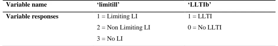
b) Limiting long-term illness (LLTI)

LLTI was re-coded to create a binary outcome whereby respondents either had a LLTI or did not. As

a binary outcome, this variable can be used in binary logistic regression. It was assumed that all

non-responses were respondents without LLTI. The original HSE variable was consistent over time so the

[image:8.595.62.533.602.680.2]

syntax to recode LLTI can be repeated for each survey year.

Table 2: Creating the ‘LLTI’ variable

Variable name ‘limitill’ ‘LLTIb’

Variable responses 1 = Limiting LI

2 = Non Limiting LI

3 = No LI

1 = LLTI

(9)

8

c) Self-assessed general health

Similar to the LLTI variable, self-assessed general health was simplified into a binary format which is

suitable for binary logistic regression. This variable was also consistent over time so the syntax used

[image:9.595.60.536.191.273.2]

can be repeated each year. As with LLTI, non-responses were assumed to be in good health.

Table 3: Creating the ‘genhelfb’ variable

Variable name ‘genhelf2’ ‘genhelfb’

Variable responses 1 = Very good/good

2 = Fair

3 = Bad/very bad

0 = Good/Very good

1 = Less than good

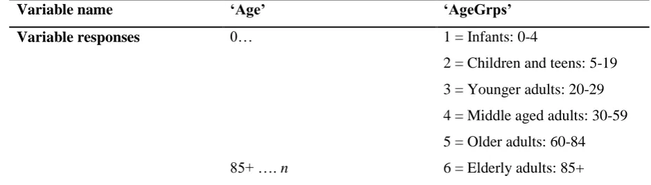
d) Age Groups

A numerical value was listed for each respondent across all survey years. This was simplified into age

groups. Boundaries for the age groups are designed to reflect natural breaks in the life course. While

arbitrary, similar groupings can be found elsewhere and these categories are suitable for the purposes

of this analysis. The syntax used can be repeated for each survey year.

Table 4: Creating Age Groups

Variable name ‘Age’ ‘AgeGrps’

Variable responses 0…

85+ …. n

1 = Infants: 0-4

2 = Children and teens: 5-19

3 = Younger adults: 20-29

4 = Middle aged adults: 30-59

5 = Older adults: 60-84

6 = Elderly adults: 85+

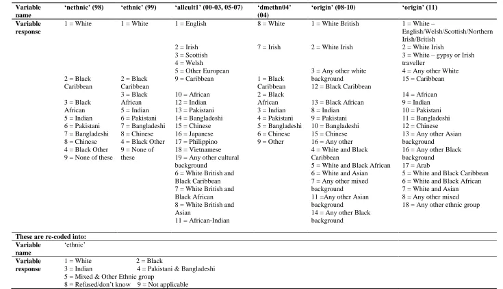
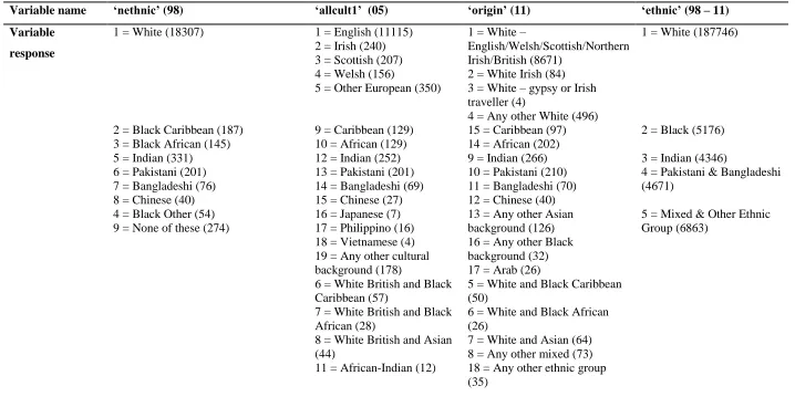
e) Ethnicity

The categorisation of ethnicity varies substantially from year to year with some years explicitly

questioning respondents about their ethnicity whilst other years chose to derive ethnicity from

respondents’ culture. Typically, those survey years which derived ethnicity from a respondent’s

culture created simplistic ethnic categories only distinguishing between White, Mixed, Black or Black

British, Asian or Asian British, and other. This is not detailed enough for the purposes of this analysis

so the original responses to the cultural questions were used to derive more detailed ethnic

[image:9.595.60.530.425.559.2]

(10)

9

Those survey years which had detailed ethnic classifications, however, also had smaller category

sample sizes which are not always suitable for statistical analysis. These were aggregated to create

larger sample sizes without becoming too heterogeneous. This is particularly important for ethnicity

as typical aggregations, such as Black and Minority Ethnic groups (BME), a commonly used ethnic

classification in health research, masks significant variation between those minority groups which

may be important for any social, economic, political or health-related analysis. Consequently,

re-coding of the ethnicity variables was based on:

a) the need to retain sufficient ethnic detail to return theoretically meaningful results;

b) the statistical necessity of large enough category sample sizes; and finally,

c) the ability to create ethnic groupings which both satisfy a) and b), but also are possible within

the constraints of the varied categorisation of ethnicity over time.

To create a harmonised ethnic variable which met the conditions described above, a number of

compromises were necessary. Firstly, it was not possible to create a ‘White British’ or even ‘White English’ grouping and aggregate all other ‘White’ in ‘Other’. This was because:

d) it was not possible to distinguish between Irish in Northern Ireland and Irish in the Republic

of Ireland even if other possible ‘ethnicity’ variables were used to cross-tabulate against. For

example, this was a problem in 2000 to 2003;

e) some survey years included a response for those who are ‘Other European’ i.e., ‘White

Other’, yet this was not consistent over time; and finally,

f) from 2008 onwards, it was not possible to distinguish between respondents who were either

‘English’, ‘Scottish’, ‘Welsh’ or ‘Northern Irish’, only those who were ‘White British’, ‘White Irish’, or ‘Any other White background’.

Secondly, due to the small numbers involved some ethnicities were combined to increase the

statistical power of the analysis:

g) ‘Black African’ and ‘Black Caribbean’ were combined to create ‘Black’; and,

h) ‘Pakistani’ and ‘Bangladeshi’ were also combined to create ‘Pakistani and Bangladeshi’.

Finally, a large heterogeneous group of ‘Mixed and Other Ethnic group’ was created to catch all of

the remaining ethnicities. These remaining categorisations were too varied year on year to create

anything more meaningful. Non-responses categorisations, as with other variables, varied between

years. Although these were ultimately excluded from the final analysis along with the mixed category,

these were initially collapsed to create two categories of either ‘Refused or don’t know’, or ‘Not

applicable’. Table 5 details the ethnicity variables used from each survey year as well as the newly

(11)

10

selects a couple of the survey years and illustrates how the categories were aggregated upwards to

give the final harmonised variable. This demonstrates the importance of collapsing some of the

categories due to the small numbers involved. For clarity, table 6 selects two of the survey years and

illustrates how the categories were aggregated to give the final harmonised variable. The final values

for the newly created ethnicity variable reflect the totals for all years and are not the sum of those

(12)

[image:12.842.50.785.98.520.2]

11

Table 5: Creating the Ethnicity variable

Variable name

‘nethnic’ (98) ‘ethnic’ (99) ‘allcult1’ (00-03, 05-07) ‘dmethn04’ (04)

‘origin’ (08-10) ‘origin’ (11)

Variable response

1 = White

2 = Black Caribbean

3 = Black African 5 = Indian 6 = Pakistani 7 = Bangladeshi 8 = Chinese 4 = Black Other 9 = None of these

1 = White

2 = Black Caribbean 3 = Black African 5 = Indian 6 = Pakistani 7 = Bangladeshi 8 = Chinese 4 = Black Other 9 = None of these

1 = English

2 = Irish 3 = Scottish 4 = Welsh

5 = Other European 9 = Caribbean

10 = African 12 = Indian 13 = Pakistani 14 = Bangladeshi 15 = Chinese 16 = Japanese 17 = Philippino 18 = Vietnamese 19 = Any other cultural background

6 = White British and Black Caribbean 7 = White British and Black African 8 = White British and Asian

11 = African-Indian

8 = White

7 = Irish

1 = Black Caribbean 2 = Black African 3 = Indian 4 = Pakistani 5 = Bangladeshi 6 = Chinese 9 = Other

1 = White British

2 = White Irish

3 = Any other white background

12 = Black Caribbean

13 = Black African 8 = Indian

9 = Pakistani 10 = Bangladeshi 15 = Chinese 16 = Any other 4 = White and Black Caribbean

5 = White and Black African 6 = White and Asian 7 = Any other mixed background

11 =Any other Asian background

14 = Any other Black background

1 = White –

English/Welsh/Scottish/Northern Irish/British

2 = White Irish

3 = White – gypsy or Irish traveller

4 = Any other White 15 = Caribbean

14 = African 9 = Indian 10 = Pakistani 11 = Bangladeshi 12 = Chinese

13 = Any other Asian background

16 = Any other Black background

17 = Arab

5 = White and Black Caribbean 6 = White and Black African 7 = White and Asian 8 = Any other mixed 18 = Any other ethnic group

These are re-coded into: Variable

name

‘ethnic’

Variable response

1 = White 2 = Black

3 = Indian 4 = Pakistani & Bangladeshi 5 = Mixed & Other Ethnic group

(13)

[image:13.842.64.782.100.468.2]

12

Table 6: Aggregating the ethnic variables

Variable name ‘nethnic’ (98) ‘allcult1’ (05) ‘origin’ (11) ‘ethnic’ (98 – 11)

Variable

response

1 = White (18307)

2 = Black Caribbean (187) 3 = Black African (145) 5 = Indian (331)

6 = Pakistani (201) 7 = Bangladeshi (76) 8 = Chinese (40) 4 = Black Other (54) 9 = None of these (274)

1 = English (11115) 2 = Irish (240) 3 = Scottish (207) 4 = Welsh (156)

5 = Other European (350)

9 = Caribbean (129) 10 = African (129) 12 = Indian (252) 13 = Pakistani (201) 14 = Bangladeshi (69) 15 = Chinese (27) 16 = Japanese (7) 17 = Philippino (16) 18 = Vietnamese (4) 19 = Any other cultural background (178)

6 = White British and Black Caribbean (57)

7 = White British and Black African (28)

8 = White British and Asian (44)

11 = African-Indian (12)

1 = White –

English/Welsh/Scottish/Northern Irish/British (8671)

2 = White Irish (84) 3 = White – gypsy or Irish traveller (4)

4 = Any other White (496) 15 = Caribbean (97) 14 = African (202) 9 = Indian (266) 10 = Pakistani (210) 11 = Bangladeshi (70) 12 = Chinese (40) 13 = Any other Asian background (126) 16 = Any other Black background (32) 17 = Arab (26)

5 = White and Black Caribbean (50)

6 = White and Black African (26)

7 = White and Asian (64) 8 = Any other mixed (73) 18 = Any other ethnic group (35)

1 = White (187746)

2 = Black (5176)

3 = Indian (4346)

4 = Pakistani & Bangladeshi (4671)

5 = Mixed & Other Ethnic Group (6863)

Note: Numbers preceding category names are the numerical values for those categories within the SPSS datasets. Numbers in brackets are the total respondents in that

(14)

13

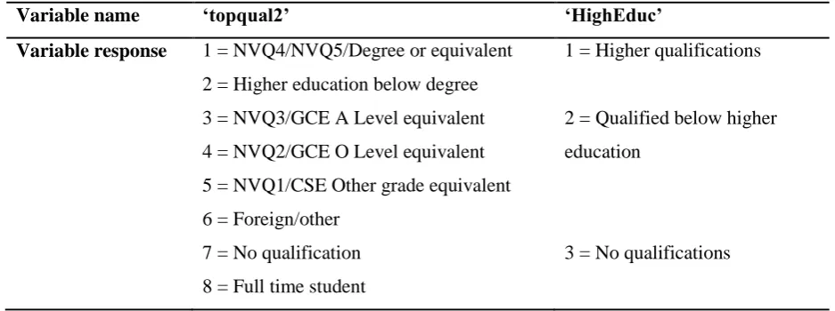
f) Educational attainment

The existing categories within the original variables covering educational attainment were collapsed

to increase the statistical power of the analysis and lead to meaningful results. ‘Foreign/Other’

qualifications are classified as below higher education as it is not possible to determine what level

[image:14.595.63.532.215.390.2]

they are equivalent to. The syntax can be repeated for each year.

Table 6: Creating the Education variable

Variable name ‘topqual2’ ‘HighEduc’

Variable response 1 = NVQ4/NVQ5/Degree or equivalent

2 = Higher education below degree

3 = NVQ3/GCE A Level equivalent

4 = NVQ2/GCE O Level equivalent

5 = NVQ1/CSE Other grade equivalent

6 = Foreign/other

7 = No qualification

8 = Full time student

1 = Higher qualifications

2 = Qualified below higher

education

3 = No qualifications

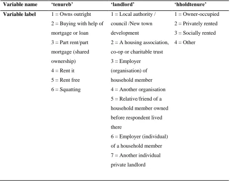
g) Household tenure

Two different variables were used to create a simplified and consistent household tenure variable.

This separately covered the nature of the tenure (tenureb) e.g. whether respondents lived in rented

accommodation, owner-occupied or lived rent free with friends, or for those who rented, who their

landlord was (landlord). The information provided in these two variables was combined to distinguish

between owner-occupied, privately rented and socially rented. To combine two separate variables, the

‘compute’ rather than the ‘recode’ function was used. The same syntax can be repeated for each

(15)

[image:15.595.66.535.100.465.2]

14

Table 7: Creating the Household tenure variable (tenureb and landlord are combined)

Variable name ‘tenureb’ ‘landlord’ ‘hholdtenure’

Variable label 1 = Owns outright

2 = Buying with help of

mortgage or loan

3 = Part rent/part

mortgage (shared

ownership)

4 = Rent it

5 = Rent free

6 = Squatting

1 = Local authority /

council /New town

development

2 = A housing association,

co-op or charitable trust

3 = Employer

(organisation) of

household member

4 = Another organisation

5 = Relative/friend of a

household member owned

before respondent lived

there

6 = Employer (individual)

of a household member

7 = Another individual

private landlord

1 = Owner-occupied

2 = Privately rented

3 = Socially rented

4 = Other

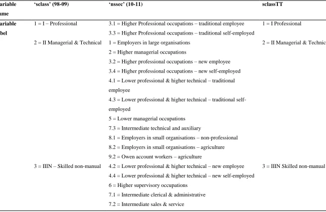
h) Social Class

Prior to 2001, the principle measure of social status or social class was the Registrar General’s Social

Class scheme. However, following calls for improvements to the theory and methods underpinning

this classification, the National Statistics Socio-economic Classification (NS-SEC) was developed.

Whilst each has their relative merits, this analysis used the RGs social class scheme. To convert the

new NS-SEC back to the RGs social class, a look-up table was used (CeLSIUS at University College

London). This was only required from 2010 onwards as up until 2009, the RGs social class was still

provided within the dataset alongside the newly established NS-SEC (which was included from

2001). All respondents who could not be classified within any one of the six social classes was

defined as ‘unclassifiable’; this also included the varying non-response categories. Table 8 details the

original social class variables, the NS-SEC variables from 2010 onwards, and the new harmonised

social class variable for the time-trend dataset. For clarity, NS-SEC categories are ordered according

(16)

15

based on the class of the head of household. Two sets of syntax were required depending on whether

(17)

[image:17.842.81.731.101.524.2]

16

Table 8: Old and New Social Class variables

Variable

name

‘sclass’ (98-09) ‘nssec’ (10-11) sclassTT

Variable

label

1 = I – Professional

2 = II Managerial & Technical

3 = IIIN – Skilled non-manual

3.1 = Higher Professional occupations – traditional employee

3.3 = Higher Professional occupations – traditional self-employed

1 = Employers in large organisations

2 = Higher managerial occupations

3.2 = Higher professional occupations – new employee

3.4 = Higher professional occupations – new self-employed

4.1 = Lower professional & higher technical – traditional

employee

4.3 = Lower professional & higher technical – traditional

self-employed

5 = Lower managerial occupations

7.3 = Intermediate technical and auxiliary

8.1 = Employers in small organisations – non-professional

8.2 = Employers in small organisations – agriculture

9.2 = Owen account workers – agriculture

4.2 = Lower professional & higher technical – new employee

4.4 = Lower professional & higher technical – new self-employed

6 = Higher supervisory occupations

7.1 = Intermediate clerical & administrative

7.2 = Intermediate sales & service

1 = I Professional

2 = II Managerial & Technical

(18)

17 4 = IIIM – Skilled Manual

5 = IV – Semi-skilled Manual

6 = V – Unskilled

7 = Armed Forces

8 = Not fully described

12.1 = Semi-routine sales

12.6 = Semi-routine clerical

7.4 = Intermediate engineering

9.1 = Own account workers – non-professional

10 = Lower supervisory occupations

11.1 = Lower technical craft

12.3 = Semi-routine technical

13.3 = Routine technical

11.2 = Lower technical process operative

12.2 = Semi-routine service

12.4 = Semi-routine operative

12.5 = Semi-routine agricultural

12.7 = Semi-routine childcare

13.1 = Routine sales & service

13.2 = Routine production

13.5 = Routine agricultural

13.4 = Routine operative

14 = Never worked & long-term unemployed

15 = Full time students

16 = Occupations not stated/inadequately described

17 = Not classifiable for other reasons

4 = IIIM Skilled manual

5 = IV Semi-skilled manual

6 = Unskilled

7 = NA/Unclassifiable (includes

armed forces, students, all who have

never worked and other

(19)

18

Save outfile =

'F:\Data\HSE\HSE_recode_FD2011. sav'

/Keep= Year age … sclassTT econact hholdtenure topqual2 carTT.

Get file = 'F:\Data\HSE\HSE_time-series.sav'. ADD FILES /FILE=*

/FILE='F:\Data\HSE\HSE_recode_2010.sav'. ADD FILES /FILE=*

/FILE='F:\Data\HSE\HSE_recode_2009.sav'. …

ADD FILES /FILE=*

/FILE='F:\Data\HSE\HSE_recode_1998.sav'. EXECUTE.

4. Extraction

Once the current survey year has been opened and the

relevant syntax to harmonise the original variables within

that year has been run, the newly created variables as well

as any to be used in their original state should be extracted

and saved into a new compressed file. This is done for each

survey year. An example of the syntax required is listed

below, to run for alternative survey years it is just necessary

to amend the output file name.

5. Creating the time-series dataset and considerations

To combine the newly created compressed

datasets, first save the most recent file as

‘HSE_time-series.sav’. Then use both the ‘Get File’ and ‘Add Files’ functions to open and then

append the remaining datasets.

Having created the time-series dataset it is

necessary to establish whether the combined

cross-sectional data are appropriate for use as a time-series. Here, considerations of the influence of

sample size in boost years as well as non-responses and survey weights are important as each may

have different implications for the final results.

a) Boost years

Boost years within the HSE oversample different population subgroups such as minority ethnic

groups or older members of the population. These larger sample sizes can distort or skew the results.

For the minority ethnic group boost years, this is avoided as the boost data is provided in separate

files. However, the boosted elderly groups in 2000 and 2005 are not separated from the main data. In

2000, the boost sample (n = ~ 2500) can be identified by cross-tabulating those living in an institution

by age but this is not possible in 2005. Thus, it is important to establish the extent of the influence of

the increased sample size on the overall results. No notable affect was found for 2000 but a clearly

discernible and consistent spike emerges for 2005 in rates of poor health. This may lead some to

exclude these two survey years, as authors of the obesity study in Manchester chose to (Higgins and

Marshall, 2012). However, as the spike in poor health rates disappears when excluding people aged

65 and over, it can reasonably be attributed to the boosted sample rather than unique socioeconomic

conditions of that year. Consequently, the files are maintained within the time-series dataset and

(20)

19

influence on population health rates of an older population is interesting in light of England’s ageing

population.

b) Non-response

Reasons for non-response varied between the survey years ranging from refused to don’t know to not

applicable. For all variables, less than 0.5% of non-responses were categorised as either ‘don’t know’

or ‘refused’. These non-responses have minimal effect on the results of the analysis and are therefore

excluded. Where non-response rates within variables were high, this was due to the inapplicability of

the variable in question. For example, they were high for the social class variable as not all

respondents could be assigned a class. Excluding the non-applicable non-responses is therefore

justified as the research is only interested in the influence of known socioeconomic attributes on

population health.

For the dependent variables, however, non-responses were included but not as non-responses. As the

dataset is based on a health survey it is likely that respondents would be predisposed to affirm if they

suffered poor health. Consequently, it is assumed that any non-response meant that the respondent

was not in poor health. Such assumptions cannot be readily made about the independent variables.

c) Survey weights

When analysing social survey data, operational decisions must be made regarding the use of weights

and choices are generally study dependent. Weights are introduced into survey data to either enhance

the representativeness of a sample (design weights), account for atypical non-respondents which can

bias an otherwise representative sample (non-response weights), or to produce results which mimic

those which would be achieved if the sample size was the same size of the total population (grossing).

Prior to 2003, the only weights within the HSE were design weights used to account for

under-sampled children aged 2 – 15 years. However, from 2003 onwards the HSE introduced non-response

weights to match developments in other large-scale datasets and try and reduce possible non-response

bias (for further information, see the 2003 HSE User Guide available in the documentation folder for

this dataset).

To test whether including weights was advisable, data were extracted and harmonised for the years

2003 and 2011, first with weights and then without. The statistical tests to be used within the

subsequent analysis were then run on each extract. Across each of the datasets, cross-tabulations by

the dependent variables and ethnicity and the remaining independent variables revealed similar

patterns. Weighting the data did not influence the conclusions drawn regarding the associations

between the variables. Similarly, four regression models were run for 2003 and 2011 with the

(21)

20 USE ALL.

COMPUTE filter_$=(Year > 1997) AND (Year < 2001).

VARIABLE LABELS filter_$ 'Year = 1996-98 (FILTER)'.

VALUE LABELS filter_$ 0 'Not Selected' 1 'Selected'.

FORMATS filter_$ (f1.0). FILTER BY filter_$. EXECUTE.

LOGISTIC REGRESSION VARIABLES LLTIb /METHOD=ENTER sex AgeGrps ethnic /Contrast (sex) = Indicator(1)

/Contrast (AgeGrps) = Indicator(1) /Contrast (ethnic) = Indicator(1) /PRINT=CI(95)

/CRITERIA=PIN(0.05) POUT(0.10) ITERATE(20) CUT(0.5).

demographic and socioeconomic attributes. The direction and size of the effects across the models are

such that you would make the same conclusions about the variable and the gradients and relationships

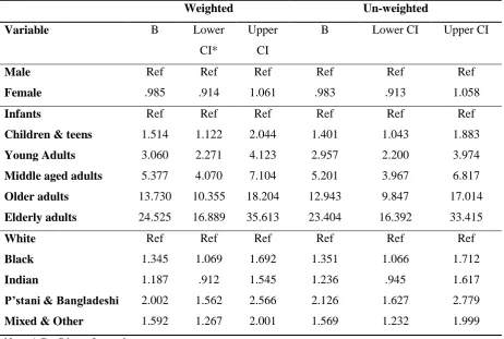
between them. This is illustrated in table 9 which shows the beta coefficients and confidence intervals

(CI) for each variable using weighted and un-weighted data using the model for less than good health

[image:21.595.68.531.225.536.2]

controlling for demographic attributes in 2003.

Table 9: Binary Logistic Regression Model for 2003, comparing weighted and un-weighted

results.

Weighted Un-weighted

Variable B Lower

CI*

Upper

CI

B Lower CI Upper CI

Male Female Ref .985 Ref .914 Ref 1.061 Ref .983 Ref .913 Ref 1.058 Infants

Children & teens

Young Adults

Middle aged adults

Older adults Elderly adults Ref 1.514 3.060 5.377 13.730 24.525 Ref 1.122 2.271 4.070 10.355 16.889 Ref 2.044 4.123 7.104 18.204 35.613 Ref 1.401 2.957 5.201 12.943 23.404 Ref 1.043 2.200 3.967 9.847 16.392 Ref 1.883 3.974 6.817 17.014 33.415 White Black Indian

P’stani & Bangladeshi

Mixed & Other

Ref 1.345 1.187 2.002 1.592 Ref 1.069 .912 1.562 1.267 Ref 1.692 1.545 2.566 2.001 Ref 1.351 1.236 2.126 1.569 Ref 1.066 .945 1.627 1.232 Ref 1.712 1.617 2.779 1.999

Note: * Confidence Interval.

6. Analysis

The time-series dataset is now ready for

analysis. Trends were explored using

rolling-three year pooled figures. Pooling the data

for each variable across rolling three-yearly

time points increases the sample sizes

involved. Filters applied to the dataset select

the required variables from the appropriate

years before each test is run, whether these

(22)

21

distributions (e.g. the count and proportion of respondents in poor health or belonging to different

social classes over time), cross-tabulations (e.g. the proportion of respondents in poor health by social

class over time) and finally, binary logistic regression models to assess how the socioeconomic and

demographic variables differently explain poor health (whether in terms of LLTI or less than good

health) over time. For clarity, this is exemplified below for binary logistic models estimating the

likelihood of LLTI in 1998 to 2000. This model only controls for the demographic variables, i.e.

ethnicity, age and gender.

The ‘Use All’ function clears any existing filters and should be run before any new filter is applied.

Filters are then computed: in the above example the syntax is commanding SPSS to only use data

from years which are greater than 1997 and less than 2001, i.e. the three year period 1998 to 2000.

The second section of the syntax commands SPSS to run a binary logistic regression model whereby

the outcome is the presence of LLTI and the demographic variables are the explanatory variables.

‘Indicator(1)’ informs SPSS that the variables are categorical and that the first category should be

used as the reference. For gender, males are the first category in the sex variable so this is the

reference. Similarly, for ethnicity, White is the first and therefore reference category. Results

presented will therefore always be illustrating what the odds of developing a LLTI in 1998 to 2000 are

for the different demographic groups compared to the relevant reference category, e.g. what are the

odds of females reporting LLTI compared to males? This example of syntax can be amended, altering

either the years, the outcome (e.g. it could be the probability of reporting less than good health), or the

explanatory variables (e.g. different combinations of demographic and/or socioeconomic variables). It

should be noted that if using SPSS to run binary logistic regression models, SPSS can only select

either the first or last variable category as the reference category. If a different category was more

appropriate to use as the reference, the variable would need to be re-coded such that this category

(such as the mode) was either the first or last.

Conclusion

This document can be read in two ways. On the one hand, it is a technical note detailing some of the

key methodological steps taken to create a time-series dataset from the HSE for the analysis of change

in the composition and structure of England’s society. On the other hand, it could be used as a general

technical guide on the steps needed to create a time-series dataset from a repeated annual survey using

SPSS. In both cases, however, the reader should remember a few caveats. Many of the steps taken,

particularly in terms of the harmonising of variables, must be understood within the context of the

research that this dataset was created for. This is important when thinking about variables which differ

substantially year on year or those where the number of variable categories leads to small sample

sizes. Additionally, the types of statistical tests to be run will also have an impact on how variables

(23)

22

requiring a binary coded format for the dependent variables, this may not be necessary for alternative

forms of analysis. These caveats hopefully remind the reader that this document is not strictly

prescriptive of what one must do to create a time-series dataset; rather it is illustrative of the kind of

steps which could be undertaken and demonstrates how these steps are carried out in SPSS using

(24)

23

Bibliography

CeLSIUS, ‘Mapping NS-SEC to Social Class’ http://celsius.lshtm.ac.uk/modules/socio/se040302.html [Accessed June 2013].

Chandola, T., (2012) ‘Spatial and social determinants of urban health in low-, middle- and high-income countries’, Public Health, 126 (3): 259-261.

Collier, J., (2010) Using SPSS Syntax: A Beginner’s Guide. Sage Publications: London.

Erens, P. and Primatesta, P., (eds) (1999) The Health Survey for England 1998: Cardiovascular Disease 1998. The Stationary Office: London.

Higgins, V. & Marhsall, A., Health Survey for England Time Series Dataset, 1991 – 2009 [computer

file]. Colechester, Essex: UK Data Archive [distributor], July 2020. SN: 7025.

Jowit, J., (2013) ‘Britain’s ageing population: the impact on families and services’ The Guardian:

http://www.theguardian.com/society/2013/feb/24/ageing-population-impact-families-services

[accessed October 2013].

Nazroo, J., (2006) ‘Ethnic Inequalities in Health’, eLS. DOI: 10.1002/9780470015902.a0005858

National Centre for Social Research and University College London. Department of Epidemiology and Public Health, Health Survey for England, 2003 [computer file]. 2nd edition. Colchester, Essex: UK Data Archive [distributor], April 2010. SN: 5098. DOI:10.5255/UKDA-SN-5098-1

Norman, P., Boyle, P., Exeter, D., Feng, Z. & Popham, F., (2011) ‘Rising premature mortality in the UK’s persistently deprived areas: Only a Scottish phenomenon?’, Social Science & Medicine, 73: 1575-1584.

Office for National Statistics, (2012) ‘Ethnicity and National Identify in England and Wales 2011’,

http://www.ons.gov.uk/ons/dcp171776_290558.pdf [accessed January 2013].

Office for National Statistics (2013) ‘Full report – Graduates in the UK Labour market 2013’,

http://www.ons.gov.uk/ons/dcp171776_337841.pdf [accessed November 2013].

Orwell, G., (1984) Why I Write. Penguin Books: London.

Shaw, M., Dorling, D., Gordon, D. & Davey Smith, G. (2004), ‘The widening gap: health inequalities and policy in Britain’, in P Boyle, S Curtis, E Graham & E Moore (Eds), The geography of health inequalities in the developed world (pp. 77-100). Aldershot: Ashgate.

Sproston, K. and Mindell, J., (2006) Health Survey for England 2004: The Health of Minority Ethnic Groups. The Information Centre: London.

(25)

24

Appendix A: Syntax

The syntax presented is primarily for the extraction, harmonisation and creation of the new time-series

dataset. It is presented in a linear format and can therefore be copied, pasted and ran if the file names

and pathways used are the same as those shown here. It should be noted that due to the coding of

ethnicity between 2005 and 2007, additional syntax was needed to create the final harmonised

variable - this is documented below. For illustrative purposes, an example of the syntax used to run

one set of binary logistic regression models for the study period is also provided. For clarity, each line

is broken up with a starred comment briefly describing what follows. This can be copied into the

syntax editor as SPSS recognises anything prefixed with a * as a line of comments.

1. Opening dataset, harmonising appropriate variables, extracting all variables of interest to new compacted dataset.

*open file.

GET FILE='F:\Data\HSE\HSE 1998\UKDA-4150-spss\spss\spss12\hse98ai.sav'.

*survey year.

COMPUTE Year = 1998.

VARIABLE LABELS Year 'Survey Year'.

EXECUTE.

*age groups

RECODE age (0 thru 4 = 1) (5 thru 19 = 2) (20 thru 29 = 3) (30 thru 59 = 4) (60 thru 84 = 5) (ELSE = 6) INTO AgeGrps.

VARIABLE LABELS AgeGrps 'simplified '.

add value labels AgeGrps

1 "Infants: 0-4"

2 "Children and teens: 5-19"

3 "Younger adults: 20-29"

4 "Middle aged adults: 30-59"

5 "Older adults: 60-84"

6 "Elderly adults: 85+".

*ethnicity.

RECODE nethnic (1=1) (2 thru 3 = 2) (5=3) (6 thru 7 = 4) (8 thru 9= 5) (4 = 5) (-6 = 9) (-9 thru -7=8) (-6 = 9) (-2 thru -1= 9) INTO ethnic.

VARIABLE LABELS ethnic 'harmonised ethnicity'.

add value labels ethnic

1 "White"

2 "Black"

3 "Indian"

4 "Pakistani and Bangladeshi"

5 "Mixed and Other ethnic group"

8 "Refused dont know"

9 "Not applicable".

*binary LLTI.

RECODE limitill (1=1) (ELSE = 0) INTO LLTIb.

VARIABLE LABELS LLTIb 'harmonised binary LLTI'.

(26)

25 1 "LLTI"

0 "no LLTI".

*binary general health.

RECODE genhelf2 (1 = 0) (ELSE = 1) into genhelfb.

VARIABLE LABELS genhelfb 'binary simplified general health'.

add value labels genhelfb

1 "Less than good"

0 "Good / Very good".

*social class.

RECODE sclass (1=1) (2=2) (3=3) (4=4) (5=5) (6=6) (ELSE = 7) into sclassTT.

VARIABLE LABELS sclassTT 'harmonised individual sclass'.

add value labels sclassTT

1 "I Professional"

2 "II Managerial and technical"

3 "IIIN Skilled non-manual"

4 "IIIM Skilled manual"

5 "IV Partly skilled"

6 "V Unskilled"

7 "NA/Unclassifiable".

*household tenure.

COMPUTE hholdtenure = 4.

if (tenureb > 0) and (tenureb < 4) hholdtenure = 1.

if (landlord > 2) and (landlord < 8) hholdtenure = 2.

VARIABLE LABELS hholdtenure 'simplified housing tenure'.

add value labels hholdtenure

1 "owner-occupied"

2 "privately rented"

3 "socially rented"

4 "other".

*car.

recode car (1 = 1) (2 = 2) (ELSE = 0) INTO carTT.

VARIABLE LABELS carTT 'harmonised car availability'.

add value labels carTT

1 "yes car available"

2 "not available"

0 “refused dont know”.

*education.

RECODE topqual2 (1 thru 2 = 1) (3 thru 6 = 2) (ELSE = 3) into HighEduc.

VARIABLE LABELS HighEduc 'simplified education: higher or not'.

add value labels HighEduc

1 "Higher qualifications"

2 "Qualified below higher education"

3 "No qualifications".

*extraction.

SAVE OUTFILE =

'F:\Data\HSE\HSE_recode_FD1998.sav'

/Keep=

(27)

26 age

AgeGrps

sex

ethnic

LLTIb

limitill

genhelf

genhelfb

sclassTT

econact

hholdtenure

HighEduc

carTT.

*open file.

GET FILE='F:\Data\HSE\HSE 1999\UKDA-4365-spss\spss\spss12\hse99gp3.sav'.

*survey year.

EXECUTE.

*age groups.

VARIABLE LABELS AgeGrps 'simplified age groups'.

1 "Infants: 0-4"

*ethnic.

RECODE ethnich (1 = 1) (2 thru 3 = 2) (5 = 3) (6 thru 7 = 4) (8 thru 9 = 5) (4 = 5) (-6 = 9) (-9 thru -7=8) (-6 = 9) (-2 thru -1= 9) INTO ethnic.

1 "White"

2 "Black"

3 "Indian"

9 "Not applicable".

*binary LLTI.

add value labels LLTIb

1 "LLTI"

0 "no LLTI".

(28)

27 VARIABLE LABELS genhelfb 'binary

simplified general health'.

1 "Less than good"

*social class.

RECODE sclass (1=1) (2=2) (3=3) (4=4) (5=5) (6=6) (ELSE = 7) into sclassTT.

1 "I Professional"

6 "V Unskilled"

*tenure.

1 "owner-occupied"

3 "socially rented"

4 "other".

*car.

RECODE car (1 = 1) (2 = 2) (ELSE = 0) INTO carTT.

2 "not available"

*education.

*extraction.

SAVE OUTFILE =

'F:\Data\HSE\HSE_recode_FD1999gp3.sav'

/Keep=

Year

age

AgeGrps

sex

ethnic

LLTIb

(29)

28 genhelf

genhelfb

sclassTT

econact

hholdtenure

HighEduc

carTT.

*open file.

*survey year.

EXECUTE.

*age groups.

1 "Infants: 0-4"

*ethnicity.

RECODE allcult1 (1 thru 5 = 1) (9 thru 10 = 2) (12 = 3) (13 thru 14 = 4) (6 thru 8 = 5) (11 = 5) (15 thru 19 = 5) (-6 = 9) (-9 thru -7 = 8) (-6 = 9) (-2 thru -1 = 9) INTO ethnic.

1 "White"

2 "Black"

3 "Indian"

9 "Not applicable".

*binary LLTI.

1 "LLTI"

0 "no LLTI".

1 "Less than good"

(30)

29 RECODE sclass (1 = 1) (2 = 2) (3 = 3) (4 = 4) (5 = 5) (6 = 6) (Else = 7) into sclassTT.

1 "I Professional"

6 "V Unskilled"

*tenure.

1 "owner-occupied"

3 "socially rented"

4 "other".

*car.

2 "not available"

*education.

*extraction.

SAVE OUTFILE =

/Keep=

Year

age

AgeGrps

sex

ethnic

LLTIb

limitill

genhelf

genhelfb

sclassTT

econact

(31)

30 HighEduc

carTT.

*open file.

*survey year.

EXECUTE.

*age groups.

1 "Infants: 0-4"

*ethnicity.

1 "White"

2 "Black"

3 "Indian"

9 "Not applicable".

*binary LLTI.

1 "LLTI"

0 "no LLTI".

1 "Less than good"

*social class.

RECODE sclass (1= 1) (2 = 2) (3 = 3) (4 = 4) (5 = 5) (6 = 6) (ELSE = 7) into sclassTT.

(32)

31 add value labels sclassTT

1 "I Professional"

6 "V Unskilled"

*tenure.

1 "owner-occupied"

3 "socially rented"

4 "other".

*car.

2 "not available"

*education.

*extraction.

SAVE OUTFILE =

/Keep=

Year

age

AgeGrps

sex

ethnic

LLTIb

limitill

genhelf

genhelfb

sclassTT

econact

hholdtenure

HighEduc

carTT.

(33)

32 GET FILE='F:\Data\HSE\HSE

2002\UKDA-4912-spss\spss\spss12\hse02ai.sav'.

*survey year.

EXECUTE.

*age groups.

1 "Infants: 0-4"

*ethnicity.

1 "White"

2 "Black"

3 "Indian"

9 "Not applicable".

*LLTI recode.

1 "LLTI"

0 "no LLTI".

1 "Less than good"

*social class.

RECODE sclass (1 = 1) (2=2) (3=3) (4=4) (5=5) (6=6) (ELSE = 7) into sclassTT.

1 "I Professional"

(34)

33 6 "V Unskilled"

*tenure.

1 "owner-occupied"

3 "socially rented"

4 "other".

*car.

2 "not available"

*education.

*extraction.

SAVE OUTFILE =

/Keep=

Year

age

AgeGrps

sex

ethnic

LLTIb

limitill

genhelf

genhelfb

sclassTT

econact

hholdtenure

HighEduc

carTT.

*open file.

*survey year.

(35)

34 *age groups.

1 "Infants: 0-4"

*ethnicity.

1 "White"

2 "Black"

3 "Indian"

9 "Not applicable".

*binary LLTI.

1 "LLTI"

0 "no LLTI".

1 "Less than good"

*social class.

recode sclass (1 = 1) (2 = 2) (3 = 3) (4 = 4) (5 = 5) (6 = 6) (ELSE =7) into sclassTT.

1 "I Professional"

6 "V Unskilled"

*tenure.

(36)

35 if (landlord > 2) and (landlord < 8)

hholdtenure = 2.

1 "owner-occupied"

3 "socially rented"

4 "other".

*car.

2 "not available"

0 "refused dont know".

*education.

*extraction.

SAVE OUTFILE =

/Keep=

Year

age

AgeGrps

sex

ethnic

LLTIb

limitill

genhelf

genhelfb

sclassTT

econact

hholdtenure

HighEduc

carTT.

*open file.

GET FILE='F:\Data\HSE\HSE 2004\UKDA-5439-spss\spss\spss14\hse04gpa.sav'.

*survey year.

EXECUTE.

*age groups.