Coupling stochastic methods and detailed dynamic simulation programs for model calibration : two preliminary case studies

COUPLING STOCHASTIC METHODS AND DETAILED DYNAMIC SIMULATION

PROGRAMS FOR MODEL CALIBRATION: TWO PRELIMINARY CASE STUDIES

Filippo Monari, Paul Strachan

ESRU, University of Strathclyde, Glasgow, UK

ABSTRACT

Dynamic simulation programs for energy modelling have reached a high level of detail and accuracy in representing the main phenomena that determine energy performances of buildings. Many of these programs have been subjected to numerous validation studies which have demonstrated their capability of representing reality adequately if the correct inputs are available. However, that is rarely the case and often many input variables are unknown or subject to high uncertainty making predictions quite different from reality.

To overcome this issue, probabilistic models can be used, in order to learn from field data and use such updated knowledge to improve physical models. This work proposes a framework to apply such concept and shows some interesting and promising results for two simple preliminary case studies.

INTRODUCTION

In the last few years, several studies have underlined the existing gap between predictions and reality, largely due to incorrect initial knowledge upon which models are built. Increased monitoring and post-occupancy evaluation can provide data to investigate the cause of this performance gap. Two steps are needed to improve modelling reliability. The first is to consider the different kinds of uncertainties involved and to provide reasonable bounds for the predictions. The second is to update the model when new information becomes available.

To address these steps the deterministic approach used by dynamic simulation tools needs to be augmented with the use of stochastic methods. One possible solution, described in this paper, is to couple detailed physical models with supportive probabilistic models in order to have the physical and statistical point of view complementing each other. In particular, Gaussian Process Regression (GPR) (Rasmussen and Williams, 2006) is used in a quasi-Bayesian framework in combination with the dynamic simulation program ESP-r (Clarke, 2001), to calibrate building models.

GPR has been used successfully for similar purposes mainly in other fields (Kennedy and O'Hagan, 2001, Higdon et al., 2008, Bayarri et al., 2007) and it has

been shown to be a convenient and capable method for integration with detailed physical models. In the field of building energy modelling such techniques have been applied in Heo et al., 2012 and Heo et al. 2013, where models were calibrated employing monthly data.

The objective of this paper is to demonstrate the integration of deterministic and stochastic methods to the problem of improving detailed models with the use of detailed measurement data. The proposed framework is presented through two preliminary case studies. The first investigates the heat flux through a multilayer wall. The second, studies the evolution of the inside conditions of an outdoor test box during co-heating and free-float set-ups.

METHODOLOGY

The proposed methodology follows the framework depicted in Higdon et al., 2008 and Bayarri et al., 2007. These works extend the previous formulation in Kennedy and O'Hagan, 2001, in order to treat output of high dimensionality. In particular, basis expansion is employed to project the data in a space of lower dimension, so reducing the computational effort necessary. In this work, Principal Component Analysis (PCA) (Ramsay and Silverman, 2005) is used for this purpose.

simplification is necessary in order to correctly perform the basis expansion and is acceptable if n is large enough. Let the n×m matrix Y, denote the simulation data and the n×m* matrix Y*_{, indicate} the measurement data.

To facilitate the calculations it is useful to scale and centre Y and Y*_{, in order to have a point-wise mean of} 0 and a point-wise standard deviation of 1. PCA is then applied on Y, Y* _{and eventually on} multidimensional input variables. In particular the weights calculated from the latter are used as inputs for the GPR model.

For each simulation period, yi, the resulting basis

expansion is indicated in the following equation :

y

_i

=

∑

j=1

p

k

_j

w

_{i , j}

=

K

w

_i (1) where kj is the j-th basis vector, column of the

n×p _{matrix K, p indicates the number of basis} vectors considered, wi,jis the weight relative to the

j-th basis vector for the i-th period and wi is the relative vector. It is advised to consider the principal components explaining at least 90% of the variance relative to the simulations. It is important to notice that each period depends only on the p weights in wi

and they are the real targets of the Gaussian Process Regression. In particular GPR is performed for each

m vector wj (j = 1, …, p). Similar result and

conclusions can be achieved for multidimensional inputs and observations.

To simplify the calculations, each input is normalized between [0,1]. Let the m×r _{matrix Z and the}

m*

×r _{matrix Z}* _{denote the input set respectively} for the simulations and for the observations:

Z

=

[

θ

T_i

x

_iT

⋮

⋮

θ

_mT

x

m T

]

;Z

*

=

[

θ

*T

x

_iT

⋮

⋮

θ

*T

x

_m* T

]

(2)

where xi is the vector of weights and values relative

to the s variable conditions, θi contains the t known

values of the calibration parameters as defined by the Latin Hypercube Design, θ*_{collects the t unknown} calibration parameters conditioning the real experiment and r is equal to the sum between s and t. The analysis continues following the three steps: training, calibration and inference of the difference process. In particular three models of increasing complexity are fitted to the data. The posterior knowledge gained from one step is always used as prior knowledge in performing the next one. In the following, I indicates an identity matrix of suitable order and diag(·) is the diagonal matrix operator (i.e. it represent a diagonal matrix with the given diagonal elements).

Training

This phase aims to train a GPR model over the simulations, in order to adequately emulate the physical model. That is achieved by finding the maximum a posteriori estimates (MAP), of the hyper parameters (HP) of the covariance function, as means of their posterior distributions.

The assumed model for each simulation period is:

y

i

=

f

(

z

i

)+ ϵ

(3)

Where f(zi) indicates the physical model emulator and

є is normal independent and identically distributed (i.i.d.) noise with zero mean and constant precision (i.e. inverse of the variance) λ.

A Normal-Gamma model is used to depict the likelihood of Y according to equation (3). By considering eq. (1), it results in equation (4):

p

(

Y

∣λ )∝

∏

_im₌₁

λ

n

2

_×

exp

{−λ

2

(

y

i

−

K

w

i

)

T

(

y

i

−

K

w

i

)}

(4)

Since the initial normalization of the data it seems appropriate to take a Gamma distribution with shape and rate equal to 5 (Γ(shape = 5, rate = 5)) as prior distribution for λ.

By algebraic manipulations, and assuming a Gaussian Process prior with 0 mean (since previous normalization) and covariance matrix Σj for the

weights, it is possible to integrate out such variables (Bishop, 2006). The result expressed basis-wise is eq. (5).

p

(

Y

∣λ )∝

p

( ̂

W

∣λ

,

Ρ

,

τ )∝

∏

j=1

p

∣( λ

k

T_j

_k

j

)

−1

_I

+ Σ

_j

∣

−0.5

×

exp

{−

1

2

̂

w

T_j

[( λ

k

T_j

_k

j

)

−1

_I

+ Σ

_j

]

−1

w

̂

_j

}

(5)

where Ŵ is the m×p matrix:

̂

W

=[(

K

T

_K

)

−1

K

T

_Y

]

T (6)

and ŵj is a column of Ŵ .

The parameters of the prior distribution over λ

become:

shape

=

5

+

0.5

m

(

n

−

p

)

rate

=

5

+

0.5

∑

_im₌₁

y

_iT

(

I

−

K

(

K

T

K

)

−1

K

T

)

y

_i

(7)

The m×m matrix Σjis defined by the following covariance function:

Σ

_{j ,i ,k}

=τ

−_j1

∏

_lr₌₁

ρ

_{l , j}4(zi ,l−zk , l)

2

The p marginal variances, τj, and the rp correlation parameters ρj,l(contained in the r×p matrix P), are the hyper parameters. Particularly interesting are the latter since their values can be interpreted as measure of sensitivity of the model to the relative inputs. Such HP are defined between [0, 1] and the influence of a parameter is higher for values close to 0.

To complete the formulation, it is necessary to set prior distributions for the HP. Since the initial standardization of the data, for each τi can be taken a

Γ(shape = 5, rate = 5) again, and for each ρi,l it has been decided to assume a beta distribution Β(1, 0.1) in order to encourage Automatic Relevance Determination (ARD) (Neal 1996). In particular such distribution encourages values for ρi,l close to 1 making inactive the inputs having a low influence on the output.

The joint posterior distribution for the hyper parameters and the precision is then given by :

p

(λ

,

Ρ

,

τ∣ ̂

W

)∝

∏

j=1

p

∣( λ

k

T_j

_k

j

)

−1

_I

+ Σ

_j

∣

−0.5

∗

exp

{−

1

2

̂

w

T_j

[(λ

k

T_j

_k

j

)

−1

_I

+ Σ

_j

]

−1

w

̂

_j

}×

∏

r , p_{l , j=1}

p

(ρ

_{l , j}

)×

∏

p_j=1

p

(τ

_j

)×

p

(λ)

(9)

where the last three terms are the prior probability distributions for λ and the HP.

The posterior distributions and the MAP estimates for these factors can be calculated by exploring the distribution depicted by eq. (8) with Markov Chain Monte Carlo (MCMC) algorithms. In this context the Metropolis within Gibbs algorithm (Rosenthal, 2007) has been used because of its robustness in high dimensional spaces.

For each ŵ_{j the sampling model is:}

̂

w

j

∼

N

(

0,

[(λ

k

Tj

k

j

)

−1

I

+ Σ

j

])

(10)

Once the HP have been tuned it is possible to sample form eq. (10) or predict the output of the physical model for new zi using GPR.

In the following two phases of the analysis the HP are kept fixed at their estimates and only λ is left free to vary, following the advice in Bayarri et al. (2007).

Calibration

The previously built probabilistic model is augmented with the field observations. The model used to represent each period is the same as indicated by equation (3):

y

i

*

=

f

(

z

i

*

)+ϵ

* (11)

where є* _{is normal i.i.d noise with precision λ}*_. Again, a Normal-Gamma model is employed to represent the probability of the field observations. Through similar steps as those followed in the

training phase it is possible to achieve the following expression for the likelihood:

p

( ̂

V

∣λ

,

λ

*

,

θ

*

)∝

∏

_jp₌₁

∣Ω

_i

∣

−0.5

×

exp

{−

1

2

v

̂

j T

Ω

−_j1

v

̂

_j

}

(12)

where:

̂

V

=

[

W

̂

_̂

W

*

]

;

̂

W

*

=[(

K

T

K

)

−1

K

T

Y

*

]

T (13)

Ω

_j

=

[

(λ

k

j T

_k

j

)

−1

_I

₀

0

(λ

*

k

T_j

_k

j

)

−1

_I

]

+

[

Σ

_j

Σ

*_j

Σ

*_jT

Σ

**_j

]

(14)

The m+m* _vector v̂_{j is a column of V . Σ}̂ j**and

Σj* are respectively the m

*

×m* _{covariance matrix} for the observations and the m×m* cross-covariance matrix between simulations and observations:

Σ

**_{j ,i ,k}

=τ

−_j1

∏

l=1

r

ρ

4_{j ,l}(zi ,l

* −zk , l

* )2

Σ

*_{j ,i ,k}

=τ

−_j1

∏

l=1

r

ρ

4_{j ,l}(zi ,l−zk , l

*

)2 (15)

As done in the training step, it is possible to sample from the distribution obtained by multiplying eq. (12) by the prior distributions for θ*_{, λ, λ}*_{, in order to} estimate these parameters:

p

(λ

,

λ

*

,

θ

*

∣ ̂

V

)∝

∏

_jp₌₁

∣Ω

_i

∣

−0.5

×

exp

{−

1

2

v

̂

j T

Ω

−_j1

v

̂

_j

}×

∏

_it₌₁

p

(θ

_i*

)×

p

(λ)×

p

(λ

*

)

(16)

Usually it is common choice to use a uniform prior between 0 and 1 for the parameters in θ* _(since previous normalization) and a Γ(shape, rate) distribution can be specified for λ*_{, in a similar way} as explained in eq. (7). The sampling model for

̂

v_{j is (where ŵ}*_j

is a column of Ŵj

*

):

(

w

̂

j

̂

w

j*

)

∼

N

(

(

0

0

)

,

Ω

j

)

(17)

Difference process

these aspects are represented with an additional term to the model expressed by eq. (11):

y

i*

=

f

(

z

*i

)+Δ(

x

i

)+ϵ

* (18)

Δ(xi), is the difference process and it depends only on the variable inputs xi. In particular it is represented as

multivariate Gaussian, with zero mean and n×n covariance matrix Di.. Under the assumption of eq. (18) the matrix Ωj and the definition of ŵi

* (rows of _Ŵ * _{) are modified as indicated in eq. (19) and} (20). The likelihood of the observations Y* _{is then} defined as the product of the right side of eq. (12) and the term depicted in eq. (23). It results:

Ω

_j

=

[

(λ

k

j T

k

j

)

−1

I

0

0

B

j

]

+

[

Σ

j

Σ

j

*

Σ

*_jT

Σ

**_j

]

(19)

̂

w

i*

=[(

K

T

A

i−1

K

)

−1

K

T

A

−i1

y

i*

]

T (20)

where:

B

j

=

diag

((

k

Tj

A

−i1

k

j

)

−1

;i

=

1,. ..

, m

*

)

(21)

A

i

=λ

*−1

I

+

D

i (22)

p

(

Y

*

∣λ

*

, D

)∝

∏

i=1

m*

∣

A

_i

∣

−0.5

×

exp

{

y

_iT

C

_i

y

_i

}

(23)

C

i

=

A

−i1

−

A

i−1

K

(

K

T

A

−i1

K

)

−1

K

T

A

−i1 (24)

Therefore Δ(xi) influences Ŵ* and is defined by its covariance matrix, Di, and conditional mean, Δi,

relative to the experiment and period. These elements and the matrices Ai can be calculated empirically by difference between the observations y*

i and

realizations drawn from the calibration model:

Δ

_i

=

1

b

∑

k=1

b

(

f

*_{i ,k}

−

y

_i*

)

A

_i

=

1

b

∑

i=1

b

(

f

_{i , k}*

−

y

_i*

)(

f

_{i , k}*

−

y

_i*

)

T

(25)

where f*

i,k are posterior realizations of the calibration

model, built by drawing b weights from eq. (17) and then applying eq. (1).

Equations (25) are recursively evaluated, after a certain number of iterations, inside the MCMC algorithm, by adding an additional step to the chain, and the Ŵ* conveniently updated. During such simulation only the calibration parameters are left free to change; HP and precisions are kept equal to their estimates.

It is possible that during the MCMC simulation the covariance structure of Δ(xi) grows too much, interfering with the calibration model. This can lead to multiple modes or to cancel out information gained in the former steps. To avoid this it is advised

to set as prior distributions for θ*_{, those inferred}

previously at least for the better identified parameters. For parameters whose probability mass is close to the boundaries of their intervals, less informative prior distributions can be set in order to verify if their values actually lie in those regions or if they were the results of an over-fitting of the calibration model to the data.

Finally a GPR model can be fitted to the resulting

Δi*. It could also can be useful to train a GPR model

over the marginal variances relative to the observations (diagonal elements of each Ai) in order to have more accurate characterization of the uncertainties. The resulting GPR model can then be used to produce confidence bands or eventually to improve predictions from the physical model.

EXPERIMENTS AND RESULTS

Wall

The first case study investigates the thermal properties of an external wall in a laboratory of an insulation plant production in the south of Sweden. The experiment was conducted for the EC Joint Research Centre, Institute for Energy and Transport in ISPRA, Italy, and consisted in monitoring the heat flux through a multilayer wall, as well as the external and internal temperatures conditioning the phenomenon, for one month.

The construction had three layers: a central core of gas concrete blocks (CB) of thickness 150 mm and two insulation glass fibre board (FB) of thickness 27 mm at both sides.

The room at the inside face of the wall was heated with an electric heater and a fan. Thermocouples and heat-flow meters were placed on both sides of the wall in order to measure the external and internal temperatures and the heat flux at the inside surface. The resulting dataset was composed by three time series of 1500 values with time step 0.5 hours. At the end of the experiment, samples were taken from the wall in order to determine the properties of each material. In particular, for the insulation boards were provided the data indicated in Table 1 and for the the concrete block only the density, equal to 552 ± 6 kg/m3_.

The problem involved inferring suitable values for glass fibre boards' specific heat (cpFB), gas concrete

blocks' conductivity (kCB) and gas concrete blocks' specific heat (cpcb), which could reproduce the measured heat flux through the wall.

[image:5.595.308.520.75.411.2]

Table 1

Wall - Properties for the glass fibre boards

EXTERNAL BOARD

INTERNAL BOARD

AVERAGE

Conductivity (mW/Km)

31.23±0.04 31.31±0.26 31.57±0.17 Density

(kg/m3₎

114.8±5.1 118.3±4.4 116.6±4.7

The result of the modelling process was a two zone model where the measured temperatures were imposed in the zones representing the relative environments and high convection coefficients have been set for the test wall surfaces in order to have the same temperatures for air and surface nodes. The starting values and prior distributions indicated in Table 2 have been assumed.

Table 2

Wall - Assumptions for calibration parameters

PARAMETER STARTING

VALUE

PRIOR DISTRIBUTION

kCB (W/mK) 0.12 U(0.08, 0.16)

cpCB (J/kgK) 800 U(640, 960)

cpFB (J/kgK) 840 U(672, 1008) A test set of 300 observations at the end of the dataset has been excluded from the calibration process in order to evaluate the calibrated model. Then, the steps depicted in the Methodology section have been followed.

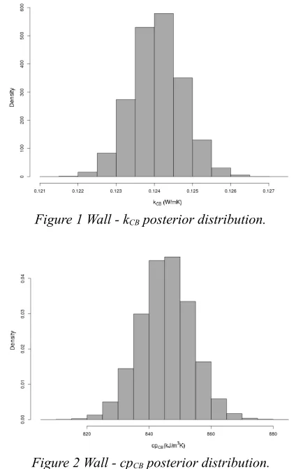
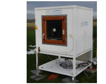
The estimates for the calibration parameters and the relative 95% confidence intervals are listed in Table 3. The empirical posterior distributions are depicted by figures 1, 2 and 3. Particularly well identified are

[image:5.595.72.289.85.179.2]

kCB and cpCB, whose posterior distributions are nicely bell shaped with low variances. The inferred distribution of cpFB, is spread all over the interval, indicating that this parameter has not been clearly identified. It is also interesting to say that at the end of the calibration step such distribution was placed against its lower bound. Considering the difference process and assuming a B(1, 2) prior for cpFB made its mean move towards the centre and the variance increase. This is reasonable considering that the sensitivity of the model to this parameter is very low and large changes in its values do not produce substantial variations in the model output.

Table 3

Wall - Calibration parameters estimates and 95% c.i.

PARAMETER ESTIMATE 95% C.I.

kCB (W/Km) 0.124 [0.123, 0.125]

cpCB (J/kgK) 845.41 [831.66, 859.07]

cpFB (J/kgK) 799.71 [731.44, 907.09] The match between the calibrated model and the observation for the test period is shown in Figure 6, while mean square errors (MSE) and the maximum

absolute errors (MAE) for training and test periods, are listed in Table 4. For this case it has been possible to achieve a particular good fit for both the training and the test data sets.

Table 4 Wall - MSE and MAE

TRAINING TEST

MSE MAE MSE MAE

ESP-r 0.007 0.29 0.017 0.36

ESP-r + Δ(x) 0.004 0.27 0.017 0.36

[image:5.595.319.516.421.570.2]

Figure 2 Wall - cpCB posterior distribution.

Figure 3 Wall - cpFB posterior distribution.

[image:5.595.307.525.644.751.2]

The difference process was very similar to an AR process with zero mean indicating that there was no significant bias in the physical model.

Test Box

The object of the second case study is a test box used in a Round Robin Experiment in the context of the International Energy Agency (IEA) Annex 58. It has cubic form with internal dimensions 96×96×96

cm3_{. The roof, floor and walls have all identical}

composition and thickness of 12 cm. One wall has a window of dimensions 60×60 cm2_{, wherein the}

glazed part has an area of 52×52 cm2_{. The whole}

structure is provided with a support which allows the influence of the ground to be neglected (Figure 5 ). The experiment, conducted at the Belgian Building Research Institute (BBRI) in Limelette, involved the monitoring of the internal conditions and the influencing weather factors for a period of 4 weeks. The experiment developed in two phases: two initial weeks where a co-heating test was performed with internal temperature of about 25 °C and a following period of two weeks in free-float set-up. For both of these tests the window was facing south.

All the data including the heat input during the co-heating phase were recorded every 5 minutes. Two comprehensive data sets were gathered comprising 31 measured variables, of 3826 and 4124 observations, for the co-heating (CH) and free-float (FF) phases respectively. For more detail the reader is referred to Jimenez et al. 2013.

The analysis has involved independent calibrations relatively to the two datasets. The first aimed to match the sensible heat load necessary to keep the inside temperature constant, and the second to reproduce the measured interior temperatures. The test set consisted in the last 800 observation of the FF data set. Two ESP-r models were built, corresponding to the two datasets. It was necessary to make assumptions about the materials' thermal properties since no information was available. Table 5 summarizes such assumptions and the prior distributions for the calibration parameters. The window was assumed to be a double glazed

construction. The thermal mass of the glass was neglected.

From each data set the following weather factors were imposed as boundary conditions on to the ESP-r models: external temperature, vertical solar radiation on the window plane, horizontal diffuse and global horizontal solar radiation, wind speed and direction, and relative humidity. In the CH model the internal temperature profile was imposed as well.

Table 5

Test box – Assumptions for the parameters

PARAMETER STARTING

VALUE

PRIOR DISTRIBUTION

Walls' conductivity (kwall ) (W/mK)

0.125 U(0.05, 0.2)

Walls' density (dwall)

(kg/m3₎

2250 U(1500, 3000)

Window's air-gap resistance (Rag)

(m2_{K/W )}

0.26 U(0.17, 0.35) Glass' normal optical

transmission (tw)

0.61 U(0.5, 0.72) Wall specific heat

(J/kgK)

800 constant

Wall emissivity 0.85 constant

Wall absorptivity 0.4 constant

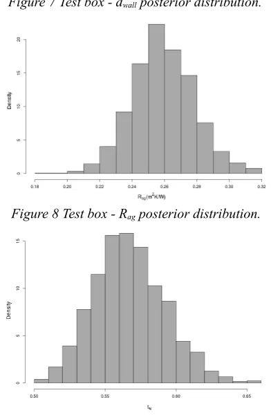
[image:6.595.315.490.70.210.2]

From the CH dataset it has been possible to infer clearly only kwall. It worth mentioning that the analysis done on the FF data returned an estimate and confidence intervals almost identical for this parameter. Table 6 summarises the main results, while figures 6, 7, 8, 9, depict the posterior distributions. All the calibration parameters are well identified with narrow confidence intervals (c.i.). Also in this case considering Δ(x) in the calibration process, changed the configuration of the predictive distributions. In particular at the end of the calibration phase, those relative to Rag and tw presented a probability mass concentrated near the lower bound of their intervals. Considering B(1, 2) prior distributions for such parameters and including the difference process in the calibration, returned

Figure 4 Wall - Comparison between test data set and calibrated model.

[image:6.595.73.287.72.219.2]

[image:7.595.320.516.38.723.2]

nicely bell shaped distributions (figures 8 and 9), actually providing a better identification for these two variables.

Table 6

Test box - Calibration parameters estimates and 95% c.i.

ESTIMATE 95% C.I.

kwall (W/Km) 0.126 [0.122, 0.130]

dwall (kg/m3) 1937 [1898.0, 1978.4]

Rag (m2K/W) 0.26 [0.23, 0.29]

tw 0.57 [0.53, 0.61]

The comparison between the prediction from the calibrated model and the data during the training and test periods are shown in figures 11 and 10. The ESP-r model seems to ESP-respond in a veESP-ry similaESP-r way to the real test box. Differences of relative significance occur in the middle of the training period and at the end of the test period. By analyzing correlations between weather factors and the difference process, it has been possible to determine that the probable causes of such differences are inadequacies in the ESP-r model in exactly representing the phenomena induced by horizontal long wave radiation. Because of this lack of the physical model, Δ(x) was not centred around zero as for the wall case, but it presented a mean of 0.46 °C. Despite this inaccuracy the calibrated ESP-r model can be considered quite accurate as indicated by its MSE and MAE (Table 7). To improve the model would be necessary to infer the sky temperature, automatically calculated in ESP-r, from the data and to consider the emissivity of the walls in the calibration.

[image:7.595.321.515.71.215.2]

Adding the difference process results in a significant better match for the training data, while relatively to the test set, it produces a lower MSE but, it does not always improves the ESP-r predictions as indicated by a relatively higher MAE (Table 7).

Table 7

Test box – MSE and MAE

TRAINING TEST

MSE MAE MSE MAE

ESP-r 0.36 0.62 0.52 1.13

ESP-r + Δ(x) 0.01 0.29 0.46 1.29

CONCLUSIONS

A framework to include field measurements in the modelling process which couples deterministic and stochastic models has been presented. According to the preliminary results the method is able to identify calibration parameters and to consider different kinds of uncertainties that lie in in both measured data and the modelling process. Although the case studies are relatively simple, nevertheless the second, is realistic

in terms of its inclusion of most of the processes determining the energy performance of the building envelope.

[image:7.595.318.515.77.378.2]

To consider the difference process in the analysis, changes the posterior distribution, especially for non dominant parameters. Its analysis can also offer

Figure 9 Test box - tw posterior distribution.

[image:7.595.70.290.119.232.2]

Figure 8 Test box - Rag posterior distribution.

Figure 6 Test box - kwall posterior distribution.

[image:7.595.318.514.374.674.2] [image:7.595.72.289.547.674.2]

insights regarding the goodness of the physical model itself, and provide information about possible improvements. At the current stage of the research it is suggested that the physical model is relied on for predictions and to use Δ(x) only for the calculation of confidence bounds. However it is believed that a full integration between the two could produce better forecasts. It is recognized that its inclusion into the MCMC algorithm might compromise the continuity of the sampling method and improving the formulation of the difference process will be the object of future research.

The true parameter values for the two cases have not been disclosed yet, but it is believed that they will be included in the inferred distributions. This statement is supported by the two good matches achieved between simulation results and metered data. ESP-r is a detailed physically-based simulation program which has been subject to extensive validation tests (Strachan et al 2007) so it is expected to be reliable for the simple cases modelled here. It is believed that using detailed simulation programs based on high quality physical models is preferable to using simplified models. In particular, it can limit, or possibly avoid, the risk of over-fitting, making the estimates dependent only on the phenomena each parameter represents. That could be very important in

future developments when will be necessary to treat more complicated models, with several parameters wherein sequential calibrations will make the analysis more feasible.

ACKNOWLEDGEMENTS

Knauf Insulation are thanked for financially supporting the construction of the IEA EBC Annex 58 round robin test box. BRE Trust are thanked for supporting the PhD research reported in this paper.

REFERENCES

Bayarri M.J., Berger J.O., Cafeo J., Garcia-Donato G., Liu F., Palomo J., Parthasarrathy R.J., Paulo R., Sacks J. and Welsh D., 2007. Computer Model Validation with Functional Output. The Annals of Statistics, 35, 1874-1906.

Bishop C.M., 2006. Pattern Recognition and Machine Learning. Springer.

Clarke J., 2001. Energy Simulation in Building Design. Butterworth-Heinemann, ISBN 978-075-065-0823.

Heo Y., Choudhary R. and Augenbroe G., 2012. Calibration of Building Energy Models for Retrofit Analysis under Uncertainty. Energy and Buildings, 47, 550-560.

Heo Y., Augenbroe G. and Choudhary R., 2013. Quantitative Risk Management for Energy Retrofit Projects. Journal of Building Performance Simulation, 6(4), 257-268.

Higdon D., Gattiker J., Williams B. and Rightley M., 2008. Computer Model Calibration Using Multidimensional Output. Journal of the American Statistical Association, 103(482), 570-583.

Jimenez M.J., Madsen H., Flamant G., Lethe G., Bauwens G., and Roels S., 2013. IEA EBC Annex 58, Subtask 3, 3rd Common Exercise on Data Analysis. Instruction Document. IEA EBC Annex 58 internal report.

Kennedy M. and O'Hagan A., 2001. Bayesian Calibration of Computer Models. Journal of Royal Statistical Society, Series B 63, 425-464. Neal, R. M., 1996. Bayesian Learning for Neural

Networks. Springer, New York. Lecture Notes in Statistics 118.

Ramsay J. and Silverman B., 2005. Functional Data Analysis. Springer

Rasmussen C. and Williams C., 2006. Gaussian Processes for Machine Learning. The MIT press. Rosenthal J.S., 2007. AMCMC: An R interface for

adaptive MCMC. Comp. Stat. & Data Anal., 51,

5467-5470.

[image:8.595.76.283.68.211.2]

Strachan P., Kokogiannakis G. and Macdonald I., 2007. History and Development of Validation with the ESP-r Simulation Program, Building and Environment (43), 601-609.

[image:8.595.72.285.251.399.2]

Figure 11 Test box – Comparison between test data set and calibrated model.