Robust control of room temperature and relative humidity using advanced nonlinear inverse dynamics and evolutionary optimisation

© CIRA, Capua, Italy 2011

ROBUST CONTROL OF ROOM TEMPERATURE AND

RELATIVE HUMIDITY USING ADVANCED NONLINEAR

INVERSE DYNAMICS AND EVOLUTIONARY OPTIMISATION

Obadah S. Zaher

Dept. of Mechanical Engineering University of Strathclyde 75 Montrose Street, Glasgow United Kingdom, G1 1XJ

Email: [email protected]

John Counsell

Dept. of Mechanical Engineering University of Strathclyde 75 Montrose Street, Glasgow United Kingdom, G1 1XJ

Email: [email protected]

Joseph Brindley

Dept. of Mechanical Engineering University of Strathclyde 75 Montrose Street, Glasgow United Kingdom, G1 1XJ

Email: [email protected]

Abstract.A robust controller is developed, using advanced nonlinear inverse dynamics (NID) controller design and genetic algorithm optimisation, for room temperature control. The performance is evaluated through application to a single zone dynamic building model. The proposed controller produces superior performance when compared to the NID controller optimised with a simple optimisation algorithm, and classical PID control commonly used in the buildings industry. An improved level of thermal comfort is achieved, due to fast and accurate tracking of the setpoints, and energy consumption is shown to be reduced, which in turn means carbon emissions are reduced.

Key words: Temperature Control, Relative Humidity, MIMO, HVAC, BEMS, Genetic Algorithm, Inverse Dynamics, Robust Control

NOMENCLATURE

𝑄 _𝑅 = Heat Transfer through Roof (W)

𝑄 𝑊 = Heat Transfer through Windows (W)

𝑄 _𝐹 = Heat Transfer through Floor (W)

𝑄 𝑓𝑟𝑒𝑒 = Heat Transfer from Free Heats (W)

𝑄 _𝑠𝑖 = Heat Transfer through internal structure (W)

𝑄 𝑠𝑒 = Heat Transfer through external structure (W)

𝑄 _𝑓𝑡 = Heat Transfer from furniture (W)

𝑇_𝑜 = Outside Temperature (K)

𝑈𝑓𝑡 = Furniture Heat Transfer Coefficient (W/m2K)

𝐴𝑠 = Area (structure) (m2)

𝐴_𝑓𝑡 = Area (furniture) (m2)

𝑀_𝑎 = Mass (air) (Kg)

𝑀_𝑠𝑒 = Mass (external structure) (Kg)

𝑀_𝑓𝑡 = Mass (furniture) (Kg)

𝐶_𝑎 = Specific Heat Capacity (air) (J/KgK)

𝐶𝑠 = Specific Heat Capacity (structure) (J/KgK)

𝐶𝑓𝑡 = Specific Heat Capacity (furniture) (J/KgK)

𝑚 𝑐 = Mass flow rate (mechanical ventilation) (Kg/s)

𝑚 𝑛𝑣 = Mass flow rate (natural ventilation) (Kg/s)

𝐾_𝑠𝑖 = Thermal Conductivity (internal structure) (W/mK)

𝑇ℎ_{𝑤𝑎𝑙𝑙} = Wall Thickness (m)

𝜌_𝑎 = Density (air) (Kg/m3)

𝑛_𝑜𝑐𝑐 = Number of occupants

𝑃_𝑜𝑐𝑐 = Evaporation rate of occupants (Kg/h)

1 INTRODUCTION

In recent years the commitment to reducing carbon emissions has led to much interest in the development of energy efficient buildings designed with a climate adaptive philosophy. These buildings incorporate sophisticated designs, materials as well as advanced Heating, Ventilation and Air Conditioning (HVAC) systems. The dynamic and uncertain nature of buildings means that designing an effective Building Energy Management System (BEMS) to control these systems is by no means a trivial task. The control methods currently in use in the buildings industry are restricted in their design to Proportional-Integral-Derivative (PID) control, as in many other industrial applications. This strategy is commonly used in industry on account of its simplicity and ease of commissioning. Many variants of PID control have been applied to HVAC systems1,2. Generally an accurate model of the plant is required in the tuning process for a PID controller. HVAC systems however, are typically nonlinear time-variable multivariable systems which are subject to many disturbances and uncertainties. Consequently, obtaining an accurate model which is representative of the plant over a wide operating range is difficult3.The tuning process for traditional PID designs can be difficult, time consuming and consequently be an expensive process particularly if re-tuning is required, as is often the case in large HVAC systems2. Poorly tuned control systems can lead to poor energy management and consequently increased carbon emissions. They also result in poor thermal comfort and can even damage actuation systems. Many advanced self-tuning PID controllers have been proposed in attempts to alleviate the problems associated with tuning PID controllers4,5. These methods however, tend to require model identification as an initial step and model parameter identification in real time mode. Hence the methods are limited due to the difficulty involved in accurately identifying such a complex process which is subjected to disturbances3,6.

Some nonlinear controller designs have been developed for HVAC systems7-9. Serrano and Reyes7 have shown that the nonlinear disturbance rejection controller is more effective at maintaining good thermal comfort levels owing to its ability to diminish the effects of thermal disturbances on the system.

temperature with HVAC systems, the sensor placement in particular has been shown to have a major effect on the performance of the control system12,13.

This paper sets forth the development of a robust and high performance controller for room temperature control of a single zone with heating through mechanical ventilation. A state of the art NID control method using Robust Inverse Dynamics Estimation (RIDE)14, which has been successful in producing robust high performance control, is used as the foundation for the controller design described in this paper. A constrained optimisation scheme using a Genetic Algorithm (GA) is employed in order to further improve the robustness characteristics of the controller by finding a set of optimal nominal gains over a range of uncertainty. The NID-GA optimal control approach has the ability to achieve fast and accurate tracking without performance degradation over a range of parameter uncertainty.

2 BUILDING MODEL

The Building model used for controller analysis in this research is based on the dynamic model developed in15,16. The zone model consists of four state variables for temperature and two state variables for humidity. These are: zone air temperature (Ta), internal wall structure temperature (Tsi), external wall structure temperature (Tse), furniture temperature (Tft), zone humidity (Wa) and relative humidity (Wrel) . The zone air is assumed to be fully mixed meaning the temperature distribution across the zone is uniform. The air density is also assumed to be constant and unaffected by changes in temperature and humidity of the zone. The differential equations that govern the zone temperature and humidity9 are as follows:

𝑀𝑎𝐶𝑎

𝑑𝑇_𝑎

𝑑𝑡 = 𝑄 𝐻 + 𝑄 𝑓𝑟𝑒𝑒 − 𝑄 𝑠𝑖− 𝑄 𝐹− 𝑄 𝑅− 𝑄 𝑊 − 𝑚 𝑐𝐶𝑎 𝑇𝑎 − 𝑇𝑜

− 𝑚 _𝑛𝑣𝐶_𝑎 𝑇𝑎 − 𝑇𝑜 − 𝑄 𝑓𝑡 (1)

𝑀_𝑠𝑖𝐶_𝑠𝑑𝑇𝑠𝑖

𝑑𝑡 = 𝑄 𝑠𝑖 − 𝐾_𝑠𝑖

𝑇ℎ_{𝑤𝑎𝑙𝑙} 𝐴𝑠(𝑇𝑠𝑖 − 𝑇𝑠𝑒) (2)

𝑀𝑠𝑒𝐶𝑠

𝑑𝑇𝑠𝑒

𝑑𝑡 = 𝐾𝑠𝑖

𝑇ℎ𝑤𝑎𝑙𝑙 𝐴𝑠 𝑇𝑠𝑖− 𝑇𝑠𝑒 − 𝑄 𝑠𝑒 (3)

𝑀_𝑓𝑡𝐶_𝑓𝑡𝑑𝑇𝑓𝑡

𝑑𝑡 = 𝑈𝑓𝑡𝐴𝑓𝑡(𝑇𝑎 − 𝑇𝑓𝑡) (4) 𝑀_𝑎

𝜌_𝑎 𝑑𝑊_𝑎

𝑑𝑡 = 𝑚 _𝑐

𝜌_𝑎 𝑊𝑠− 𝑊𝑎 +

(𝑛_𝑜𝑐𝑐𝑃_𝑜𝑐𝑐) 𝜌_𝑎 −

𝑚 _𝑛𝑣

𝜌_𝑎 𝑊𝑎 − 𝑊𝑜 (5)

𝑑𝑊𝑟𝑒𝑙

𝑑𝑡 = 5000.0𝑊 𝑎− 1.388𝑇 𝑎 (6)

When the control system is applied, the comfort temperature (Tc) is tracked which is a combination of the air, internal structure and furniture temperatures. The comfort temperature is defined as follows:

𝑇_𝑐 = 0.33𝑇_𝑎 + 0.33𝑇_𝑠𝑖 + 0.33𝑇_𝑓𝑡 (7)

heater are characterised by a nonlinear first order transfer function which has a maximum heat output of 10kW. Mechanical ventilation is provided using a fan model which is also characterised by a nonlinear first order transfer function which can provide a maximum mass flow rate of 0.35kg/s.

3 CONTROLLER DESIGN

3.1 Proportional and Integral Control

The PI controller is very commonly used in building control systems as well as many other industrial applications due to its simplistic design. For this reason, a PI controller tuned with a Nelder-Mead Simplex optimisation algorithm17 is used in this paper as a representation of current best practice in industry. This serves as a reasonable benchmark against which the advanced control method presented in this research can be compared.

The PI control law is as follows:

𝑢𝑐 𝑡 = 𝐾𝑃𝑒 𝑡 + 𝐾𝐼 𝑒(𝑡) (8)

The proportional and integral gains, KP and KI respectively, can be tuned in order to attain the best performance according to the design specifications of the system. The objective function for optimisation is taken as the root mean square of the error between the setpoint and the system response. Since there are two outputs i.e. two channels, the error is taken as the sum of the error on both channels. The objective function calculation is shown below:

𝑜𝑏𝑗 = (𝐸1+ 𝐸2… . +𝐸𝑛)

𝑛 (9)

Where E is the sum of the error on both channels and n is length of the error vector.

3.2 RIDE Control

The RIDE controller design has proven to be highly effective when applied to nonlinear systems18. An overview of the algorithm is given in this section in order to clarify the tuning problem. The algorithm is described in greater detail in14. The buildings differential equations can be represented in generalised state space format as shown in (10):

𝑥 𝑡 = 𝐴𝑥 𝑡 + 𝐵𝑢 (𝑡) (10)

𝑦 𝑡 = 𝐶𝑥 (𝑡)

The RIDE control law is given by:

𝑢𝑐

(𝑡) = 𝑟 − 𝐾_𝑃𝑦 (𝑡) + 𝑢 _𝑒𝑞(𝑡) (11)

𝑟 = 𝐾_𝐼𝑒 (𝑡) (12)

Where KP and KI are the proportional and integrals gains (which require tuning) respectively. The 𝑢 _𝑒𝑞 term (13) is an estimate of the equivalent control which is required to set rate of change of the output to zero. The equivalent control estimate uses dynamic inverse to diminish disturbances, cross-coupling and nonlinear plant dynamics. A diagram of the RIDE controller structure is shown in Fig.1

Figure 1: RIDE Controller Structure

The closed loop transfer function of the plant and control system is given by

𝐺(𝑠) = [𝑠2_𝐼

𝑚 + 𝑠 𝐾𝑃𝐶𝐵 + 𝐾𝐼𝐶𝐵]−1𝐾𝐼𝐶𝐵 (14)

Where Im is an identity matrix. The proportional and integral gains can be selected such that they are expressed as follows:

𝐾𝑃 = [𝐶𝐵]−12𝑍𝑑Ωn (15)

𝐾_𝐼 = [𝐶𝐵]−1_𝛺

𝑛2 (16)

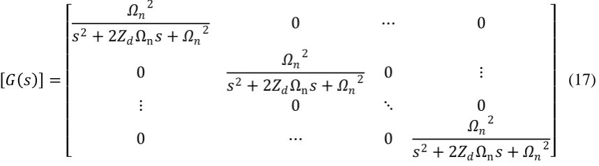
Where Zd and Ωn are the designed system damping ratio and natural frequency respectively. By setting KP and KI as in (15) and (16), the system transfer function can be expressed as a diagonal matrix of second order transfer functions in generalised form as shown below:

𝐺 𝑠 =

𝛺_𝑛2 𝑠2 _{+ 2𝑍}

𝑑Ωn𝑠 + 𝛺𝑛2

0 ⋯ 0

0 𝛺𝑛

2

𝑠2_{+ 2𝑍}

𝑑Ωn𝑠 + 𝛺𝑛2

0 ⋮

⋮ 0 ⋱ 0

0 ⋯ 0 𝛺𝑛

2

𝑠2_{+ 2𝑍}

𝑑Ωn𝑠 + 𝛺𝑛2

(17)

3.3 Genetic Algorithm Optimisation

The Genetic Algorithm is an evolutionary optimisation method based on Darwin's theory of evolution. The GA process is illustrated in the flowchart shown in Fig.2. A detailed explanation of Genetic Algorithms can be found in19.

Figure 2: GA Process20

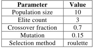
Genetic Operations:- These operations determine which individuals constitute the subsequent population. There are four operators used in the GA for this application; Elite Children, Selection, Crossover and Mutation. The settings for the GA used in the auto-tuning process are given in Table 1.

Parameter Value

Population size 10

Elite count 3

Crossover fraction 0.7

Mutation 0.15

Selection method roulette

Table 1: GA Parameters

3.3.1 Objective Function

range (Uft = 0.8W/m2K and Uft = 3.2W/m2K).

4 RESULTS

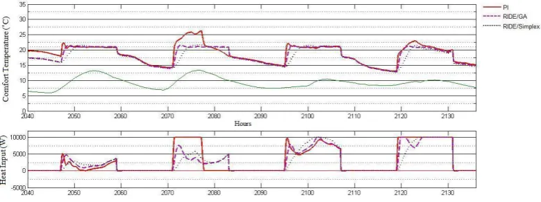
The control systems discussed above where all applied to the building model and simulated over a three month winter/spring period with weather data from January to March. Their performance was evaluated over three different operating conditions across the range of uncertainty in the heat transfer coefficient of the furniture. This was done in order to demonstrate each controller‟s ability to cope with parameter uncertainty which is very common in buildings. The different operating conditions were: Uft = 0.8W/m2K, Uft = 2.0W/m2K and Uft = 3.2W/m2K, where Uft = 2.0W/m2K is the „normal‟ operating condition.

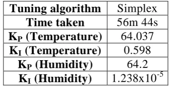
The PI controller was tuned using the aforementioned Nelder-Mead Simplex optimisation algorithm so as to provide a representation of the control systems currently in use in the buildings industry. The controller was tuned at the lower setting for the furniture heat transfer coefficient as achieving good control at this condition was found to be the most difficult. Simulation results for the RIDE controller tuned using both the simplex algorithm and the GA are also presented in order to provide a direct comparison of the efficacy of both methods. The objective function described in section 3.3.1 was used for both tuning algorithms when tuning the RIDE controller. The tuning results for all three controller setups are detailed below in Table 2 and Table 3.

Tuning algorithm Simplex

Time taken 56m 44s

KP (Temperature) 64.037

KI (Temperature) 0.598

KP (Humidity) 64.2

KI (Humidity) 1.238x10-5

Table 2: PI Auto-Tuning Results

Tuning algorithm

Simplex GA

Time taken 2h 14m 04s 42m 24s

ζ 0.7315 0.81

ω 0.000301 0.00062

Table 3: RIDE Auto-Tuning Results

Figure 3: Comfort temperature and heat input (Uft = 2.0W/m2K)

Figure 4: Relative humidity (Uft = 2.0W/m2K)

Fig. 4 shows that all three controllers track the relative humidity ratio setpoint (50%) accurately. The PI controller however can still be seen to produce some overshoot. The GA tuned RIDE controller again achieves a quick and accurate response whilst the simplex tuned RIDE controller shows a significantly slower response.

Figure 6: Relative humidity (Uft = 0.8W/m2K)

Fig.5 and Fig.6 show the response of the controllers at the lower extreme operating condition, Uft = 0.8W/m2K. The PI controller shows an improvement in tracking accuracy over the response shown in Fig.3 however, a significant level of overshoot still remains. This performance improvement can be partly attributed to the fact that the PI controller was tuned for optimum performance at this operating condition. The GA tuned RIDE controller shows a very similar response to that seen under the normal operating condition. The simplex tuned RIDE controller does however show significant performance degradation in the tracking of comfort temperature and relative humidity. This is clearly down to poor tuning on the simplex algorithms behalf since the performance of the GA tuned RIDE controller is unaffected. This highlights the efficacy of the GA for auto-tuning as well as elucidating the benefit of auto-tuning over a range of parameter uncertainty.

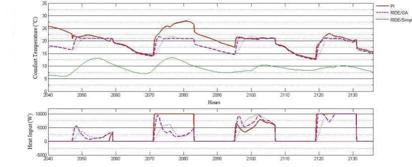
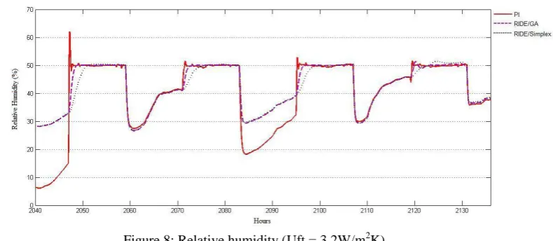
Figure 8: Relative humidity (Uft = 3.2W/m2K)

Fig.7 and Fig.8 corroborate the results observed above. The PI controller shows a severe performance degradation with very large overshoots occurring in the comfort temperature. The GA tuned RIDE controller again shows quick and accurate tracking of the setpoint in both cases whilst the simplex tuned RIDE controller has a significantly slower response time.

The total energy usage over three months under all three operating conditions for the controller setups is shown in Table 4.

Uft

(W/m2K)

RIDE/GA Energy used (W)

RIDE/Simplex Energy used

(W)

PI/Simplex Energy used

(W)

0.8 3.1368x108 2.7396x108 3.7125x108 2.0 3.1078x108 2.8915x108 3.5992x108 3.2 3.0663x108 2.8726x108 3.6397x108

Table 4: Total Energy Usage

The simplex tuned RIDE controller clearly uses less energy than the other two setups; however it produces an unsatisfactory system response. The PI controller uses substantially more energy than both RIDE controller setups. The GA tuned RIDE controller has substantially lower energy usage than the PI controller whilst maintaining very good performance under all three operating conditions.

9 CONCLUSION

It was shown in the simulation results that the RIDE control method with GA optimisation produced superior performance over the other methods tested. High performance control was achieved under all three operating conditions meaning that, in practice, a good level of thermal comfort for building occupants would be achieved as well as a reduced level of carbon emissions.

11 REFERENCES

[1] Ya-Gang Wang, Zhi-Gang Shi and Wen-Jian Cai, "PID autotuner and its application in HVAC systems", American Control Conference, vol.3, 2192-2196 (2001).

[3] H. Mirinejad, S. H. Sadati, M. Ghasemian and H. Torab, "Control Techniques in Heating, Ventilating and Air Conditioning (HVAC) Systems", J. Computer Sci., 4 (9), 777-783 (2008). [4] G. Cao, G. Tu, D. An and C. Lou, “Modeling and simulation of expert PID control for air

conditioning system based on MATLAB,” Heating Ventilating and Air Conditioning, vol.35, 111-114 (2005).

[5] Guang Qu and M. Zaheeruddin, "Real-time tuning of PI controllers in HVAC systems", Int. J. Energy Res., 28, 1313-1327 (2004).

[6] Piao Ying-Guo, Zhang Hua-Guang and Zeungnam Bien, "A simple fuzzy adaptive control method and application in HVAC," Fuzzy Systems Proceedings, IEEE World Congress on Computational Intelligence., vol.1, 528-532 (1998).

[7] B. Arguello-Serrano and M. Velez-Reyes, "Nonlinear control of a heating, ventilating, and air conditioning system with thermal load estimation," IEEE Transactions on Control Systems Technology, vol.7, 56-63 (1999).

[8] E. Semsar, M. J. Yazdanpanah and C. Lucas, "Nonlinear control and disturbance decoupling of an HVAC system via feedback linearization and back-stepping," IEEE Conference on Control Applications, vol.1, 646- 650 vol.1, 23-25 (2003).

[9] C. Rentel-Gomez and M. Velez-Reyes, "Decoupled Control of Temperature and Relative Humidity using a Variable-Air-Volume HVAC System and Non-interacting Control", IEEE Int. Conference on Control Applications, 1147-1151 (2001).

[10] L. Ding, A. Bradshaw, and C. J. Taylor, "Robustness Comparison of Control Systems for a Nuclear Power Plant", UKACC international conference on Control (2004).

[11] J. M. Counsell, J. Brindley and M. Macdonald, "Non-Linear Autopilot Design Using the Philosophy of Variable Transient Response", AIAA Guidance, Navigation and Control Conference (2009). [12] D. P. Bloomfield and D. J. Fisk, "Room thermal response and control stability", Building Serv Eng

Res Technol, vol. 2, 88-92 (1981).

[13] P. Riederer, D. Marchio, J. C. Visier, A. Husaunndee and R. Lahrech, "Influence of Sensor Position in Building Thermal Control: Development and Validation of and Adapted Zone Model", Int. IBPSA Conference, 449-456 (2001).

[14] Counsell J.M., “Optimum and Safe Control Algorithm for Modern Missile Autopilot Design”, PhD thesis, Lancaster University, 1992

[15] Murphy G B , Khalid Y , and Counsell J., “A SIMPLIFIED DYNAMIC SYSTEMS APPROACH FOR THE ENERGY RATING OF DWELLINGS”, Accepted Paper. Twelfth International IBPSA Conference, Sydney, Australia, (2011)

[16] J. M. Counsell, Y. A. Khalid and J. Brindley, "Controllability of Buildings: A input multi-output stability assessment method for buildings with slow acting heating systems", Simulation Modelling Practice and Theory, 1185-1200 (2011).

[17] MATLAB Documentation, "Optimisation ToolboxTM User's Guide", Copyright 1990 - 2009 by The MathWorks, Inc

[18] C. Fielding, A. Varga, S. Bennani and M. Selier, Advanced Techniques for Clearance of Flight Control Laws, Springer-Verlag, New York, (2002).

[19] Man K. F., Tang K. S. and Kwong S., "Genetic Algorithms: Concepts and Designs", Published by Springer-Verlag London Limited, 1999 Printed in Great Britain