Spacecraft formation flying using bifurcating potential fields

SPACECRAFT FORMATION FLYING USING BIFURCATING POTENTIAL FIELDS

Derek Bennet

Department of Mechanical Engineering, University of Strathclyde, Glasgow, Scotland

[email protected]

Colin McInnes

Department of Mechanical Engineering, University of Strathclyde, Glasgow, Scotland

[email protected]

Abstract— The distributed control of spacecraft flying in formation has been shown to have advantages over conventional single spacecraft systems. These include scalability, flexibility and robustness to failures. This paper considers the real problem of actuator saturation and shows how bound control laws can be developed that allow pattern formation and reconfigurability in a formation of spacecraft using bifurcating potential fields. In addition the stability of the system is ensured mathematically through dynamical systems theory.

I. INTRODUCTION

Recently formation flying has emerged as an enabling technology for future space systems that allows for a variety of new and exciting mission concepts. By distributing the functionality of the system over several spacecraft it has been shown that the performance can be significantly improved in comparison with a large single spacecraft[1]. At present there are several formation flying concepts currently being investigated, for example, for interferometric/sparse aperture missions. The Stellar Imager is an example of such a mission that consists of a UV/Optical deep-space telescope composed of approximately 30 one-meter array elements[2]. Another example is the DARWIN mission that will consist of6spacecraft equipped with optical telescopes in formation at the Sun-Earth L2 point[3].

Scharf et al.[4] and Lawton [5] define five formation control architectures for spacecraft formation flying; Multiple-Input, Multiple-Output (MIMO), Virtual Structure (VS), Leader/Follower (L/F), Cyclic and behavioral.

MIMO follows the multiple input, multiple output methodology, considering the relative states of the formations as a single plant[6]. The advantage of this system is that optimality can be guaranteed, however, the controller can become unstable with the failure of one spacecraft[4]. The VS system is a centralised control architecture where all spacecraft in the formation are part of a virtual rigid structure where changes in the position of each spacecraft are communicated with a formation controller and the appropriate alterations are made to the structure[7]. The system has the advantage of maintaining a formation well during manoeuvrers[8] , however, it does not perform well if the formation shape is time-varying and is also susceptible to failure as it is centralised control [9].

The L/F architecture is a centralised hierarchical control scheme where one spacecraft obtains information on a desired trajectory and follower spacecraft track the leader[10], [11]. The Landsat-7 and Earth Observing-1 (EO-1) satellites are examples of a real hierarchical L/F mission and is generally considered the first mission to demonstrate formation flying[1]. The two satellites in this formation do not communicate with each other directly. Instead a central controller determines Landsat-7’s position and sends this information to EO-1 determining the future orbits of both spacecraft[12]. The limitation of this system is that it is also dependent upon the central controller and is therefore susceptible to failure. In addition as the number of spacecraft increase, the workload required to maintain a formation discretely will increase significantly. Cyclic controller architectures are similar to the L/F however each spacecraft are connected in a non-hierarchical way[13].

A promising approach to overcome the limitations of the architectures discussed above is to develop behavioral control architectures in which all spacecraft interact producing an emergent global behaviour. One such method is the use of the artificial potential function method[14] that is used throughout this paper. This autonomous distributed system allows for agents to be driven to desired goal positions whilst ensuring collision avoidance and can be considered scalable, flexible and robust to individual spacecraft failures. It has been used successfully, for example, by Reif and Wang as a form of distributed behavioural control for autonomous robots[15], by McQuade[16] in formation flying and by Badaway and McInnes in autonomous structure assembly[17]. Related approaches have been developed by Izzo to form coherent spatial patterns in large spacecraft swarms[18].

proof. Bifurcation methods are employed to create a flexible system that can allow for different spacecraft configurations to be formed through a simple parameter changes to command the entire formation.

The paper proceeds as follows. In the next section we describe the formation model used and explain the artifi-cial potential field method and bifurcation theory. We then discuss the linear and non-linear stability of the models developed in Section III. Section Section IV shows the numerical results of simulations carried out and also control force experienced during simulation.

II. FORMATION MODEL

A. Model and Basic Formation Properties

We consider a swarm of homogeneous autonomous space-craft (1 ≤ i ≤ N) interacting via an artificial potential functionU. It is assumed that all spacecraft can communicate with each other and are fully actuated. The negative gradient of the artificial potential defines a virtual force acting on each spacecraft so that the dynamics of each spacecraft can be described by Eq. 1 and 2 with mass,m, position,xi, and velocity,vi;

dxi

dt =vi (1)

mdvi

dt =−∇iU

S_(xi)

− ∇iUR(xij)−σvi (2)

From Eq. 2 it can be seen that the virtual force experienced by each spacecraft is dependent upon the gradient of two different artificial potential functions and a dissipative term, where σ > 0 controls the amplitude of the dissipation. The first term in Eq. 2 is defined as thesteering potential,

US _{which will control the formation, whereas the second} term in Eq. 2 is the collision avoidance pairwise repulsive potential,UR_.

The repulsive potential is based on a generalized Morse potential [20] as shown in Eq. 3;

UijR=

X

j,j6=i

Crexp−|xij|/Lr (3)

where Cr and Lr represent the amplitude and length-scale of repulsive potential respectively and|xij|=|xi−xj|.

The total repulsive force on theith_{spacecraft is dependent} upon the position of all the other (N −1) spacecraft in the formation. The repulsive potential is therefore used to ensure that as the spacecraft are steered towards the goal state they do not collide with each other. Once all the spacecraft have been driven to the desired equilibrium state the repulsive potential also ensures that they are equally spaced for symmetric formations.

B. Artificial Steering Potential Function

The aim of the steering potential is to drive each spacecraft to a desired position in phase space with the repulsive potential ensuring collision avoidance and equally spaced symmetric formations. We have previously shown how this can be achieved through classical bifurcation methods in order to create a system that is capable of forming three different formations; ring, double ring and cluster through a simple parameter change assuming ideal spacecraft [21]. In order to ensure the stability of real, mission critical systems it is important to consider actuator saturation.

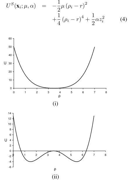
In [21] the steering potential was based on the classical pitchfork bifurcation as shown in Eq. 4 and Fig. 1 with xi = (ρi, zi)T and ρi = (x2+y2)0.5. As the gradient of this potential is unbound as the distanceρi from the origin increases the control force is also unbound and actuator saturation would occur in the system.

US(xi;µ, α) = −₂1µ(ρi−r)2

+1

4(ρi−r)

4

+1 2αz

2

i (4)

0 10 20 30 40 50 60

0 1 2 3 4 5 6 7 8

ρ U

(i)

-6 -4 -2 0 2 4 6 8 10 12 14

0 1 2 3 4 5 6 7 8

ρ U

[image:2.612.324.543.257.565.2]

(ii)

Fig. 1. Potential functions: (i)µ <0_{and (ii)µ >}0

a bound control force, where the constant Ch controls the amplitude of the function;

Uh(ρi) =Ch(ρi−r)2+ 1

0.5

(5)

0 1 2 3 4 5 6

0 1 2 3 4 5 6 7 8 9 10

ρi

[image:3.612.224.530.39.519.2]

Uh

Fig. 2. Hyperbolic Potential Function (Ch= 1,r= 5)

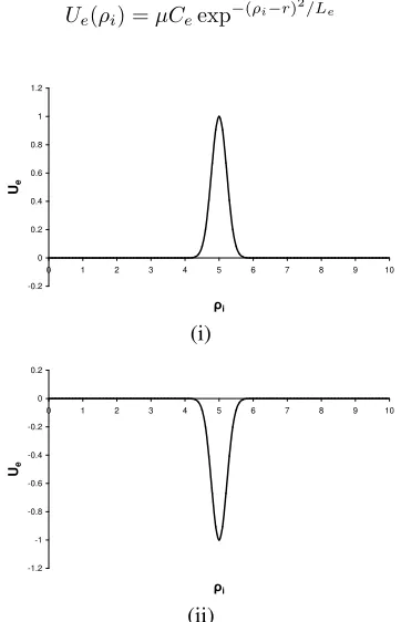
[image:3.612.58.246.44.200.2]

In order to make use of the principles demonstrated through the pitchfork bifurcation we can add an additional exponential potential function,Ue(ρi), shown in Eq. 6 and Fig. 3 that has amplitude Ce, range Le, and bifurcation parameterµ;

Ue(ρi) =µCeexp−(ρi−r)

2_/L

e ₍₆₎

-0.2 0 0.2 0.4 0.6 0.8 1 1.2

0 1 2 3 4 5 6 7 8 9 10

ρi

Ue

(i)

-1.2 -1 -0.8 -0.6 -0.4 -0.2 0 0.2

0 1 2 3 4 5 6 7 8 9 10

ρi

Ue

(ii)

Fig. 3. Exponential potential function (Ce = 1,Le = 1, r= 5): (i) µ >0_{(ii)µ <}0

Combining Eq. 5 and 6 together we achieve the bound steering potential given in Eq. 7 with Fig. 4 and Fig. 5 showing the bifurcation diagram and potential of this equation. The last term in Eq. 7 ensures that the formation is created in the x-y plane driving the z-position coordinate to zero.

US(xi) = Uh(ρi) +Ue(ρi)

= Ch(ρi−r)2+ 1

0.5

+µCeexp−(ρi−r) 2

/Le

+Cz

z2i + 1

0.5

(7)

0 1 2 3 4 5 6 7 8 9 10

-6 -4 -2 0 2 4 6 8

ρeq

µ

Stable Unstable

Stable

[image:3.612.302.507.235.480.2]

Stable

Fig. 4. Steering potential bifurcation diagram (Ch= 1,r= 5,Ce= 1, Le= 1)

0 1 2 3 4 5 6

0 1 2 3 4 5 6 7 8 9 10

ρi

U

s

(i)

0 1 2 3 4 5 6

0 1 2 3 4 5 6 7 8 9 10

ρi

U

s

(ii)

Fig. 5. Steering potential function (ρdirection): (i)US

h:µ≤0,Ch= 1, Ce = 1,Le = 1,r= 5(ii) UhS:µ >0,Ch= 1,Ce = 3,Le = 1, r= 5

III. STABILITY

A. Artificial Potential Function Scale Separation

As noted in the previous section the force experienced by each spacecraft is dependent upon the gradient of two different artificial potential functions both of which are dependent upon position;

US _{= C}

h(X−r)2+ 1

0.5

+µCeexp−(X−r) 2

/Le

(8)

[image:3.612.69.250.292.573.2]

For illustration we consider a simple 1-dimensional system with position coordinateX.

Defining an outer region dependent upon the steering potential only and an inner region dependent upon the repulsive potential only we can show that these two regions are separated so that the spacecraft move under the influence of the long-range steering potential, but with short range collisions (for Lr/R <<1) effectively creating a boundary layer between them. This can then be used to determine the non-linear stability of the formation using the steering potential only.

For 1D motion of a spacecraft of massmwe have;

mdV

dt = −

∂UR

∂X −

∂US

∂X −σV (10)

so that,

mV dV

dX =

Cr

Lr

exp−X/Lr₋ Ch(X−R)

[(X−R)2_{+ 1]}0.5

+2µCe

Le

(x−r) exp−(X−R)2/Le_−σV

(11)

ScalingX such thatS=X/Rthen;

1

RmV

dV

dS =

Cr

Lr

exp−

R

LrS

+R(S−1)

_2µC

e

Le

exp−(SR−R)2

Le

− Ch

[(SR−R)2_{+ 1]}0.5

#

−σV (12)

Now defineε=Lr

R <<1 so that;

mVdV

dS =

Cr

ε exp

−S

ε

+R 



R(S−1) 

 

2µCe

Le

exp−

(SR−R)2

Le

− Ch

[(SR−R)2_{+ 1]}0.5

!

−σV #

(13)

Letε→0in order to consider ‘far field’ dynamics which forms a singularly perturbed system and note that;

lim ε→0

1

εexp



−

S ε





= 0 (14)

Therefore at large separation distances the repulsive potential vanishes and we can consider the steering potential

only when considering the stability of analysis of the system.

Conversely if we define S = S

ε we find that the ‘near

field’ dynamics are defined by;

mVdV

dS = Crexp

−S

+ǫR

R(S−1)

_2µC

e

Le

exp−(SR−R)2

Le

− Ch

[(SR−R)2_{+ 1]}0.5

!

−σV #

(15)

and lettingε→0;

mVdV

dS =Crexp

−S ₍₁₆₎

Thus, at small separations the steering potential vanishes and we can treat the collisions separate in the subsequent stability analysis.

Also if we consider a spacecraft to be moving at its maximum speedVmtowards another spacecraft and assume that the spacecraft needs to brake toV = 0atS =Xmin/Lr we have;

m

Z 0

Vm

V dV = Cr

Z S

∞

exp−SdS (17)

so that,

−1₂mVm2 = −Crexp−S S

∞ (18)

The minimum separation is then estimated as;

Xmin = Lrln

2Cr

mV2

m

(19)

Therefore, we can assure collision avoidance with the condition that2Cr > mV2

m.

B. Linear Stability

In order to determine the linear stability of a system of spacecraft subject to such a1-parameter bifurcation steering potential we perform an eigenvalue analysis on the linearized equations of motion assuming that at large separation dis-tances the repulsive potential can be neglected through scale separation as explained in section II A. The linear stability analysis will be used to determine the local behaviour of the system by calculating its eigenvalue spectrum. Therefore, the equations of motion for the model are re-cast as;

˙

xi ˙

vi

=

vi

−σvi− ∇iUS(xi)

=

f(xi,vi)

g(xi,vi)

(20)

f(xo,vo) = 0 (21)

g(xo,vo) = 0 (22)

Defining δxi = xi−xo and δvi = vi−vo and Taylor Series expanding about the fixed points to linear order the eigenvalues of system can be found using;

δx˙i

δv˙i

=J

δxi

δvi

(23)

where,

J=

∂

∂xi(f(xi,vi))

∂

∂vi(f(xi,vi))

∂

∂xi(g(xi,vi))

∂

∂vi(g(xi,vi))

xo,vo

(24)

The Jacobian,J, is then a4x4 matrix given by;

J=     

0 0 1 0

0 0 0 1

−∂∂ρ2U2

i −

∂2_U

∂ρi∂zi −σ 0

−∂ρ∂2i∂zUi −

∂2_U ∂z2

i 0 −σ

     ˜

xo,vo

(25)

Substituting a trial exponential solution into Eq. 23 we find that;

δxi

δvi

=

δxo

δvo

eλt ₍₂₆₎

Therefore, the eigenvalues, λ, of the system are found fromdet(J₋λI) = 0.

For µ < 0 (Ch = 1, Ce = 1, Le = 1 and r = 5)

equilibrium of Eq. 20 occurs when ρeq = 5, zeq = 0 and

veq = 0. Evaluating the Jacobian matrix given in Eq. 25 with

µ=−2,σ= 2 we find that;

J=



  

0 0 1 0

0 0 0 1

−5 0 −2 0 0 −1 0 −2



  

(27)

The corresponding eigenvalue spectrum is then;

λ = −1 ± i,−1,−1. As the eigenvalues are either negative real or complex with negative real part the equilibrium position can be considered linearly stable.

For µ > 0 (Ch = 1, Ce = 1, Le = 1 and r = 5)

equilibrium occurs when; ρeq1 = 5, ρeq2 = 3.61, ρeq3 =

6.39,zeq= 0andveq = 0. The Jacobian matrix evaluated at the three different equilibrium positions is given by Eq. 28, 29 and 29.

J1=



  

0 0 1 0

0 0 0 1

3 0 −2 0 0 −1 0 −2



  

(28)

J2=



  

0 0 1 0

0 0 0 1

−1.86 0 −2 0 0 −1 0 −2



  

(29)

J3=



  

0 0 1 0

0 0 0 1

−1.86 0 −2 0 0 −1 0 −2



  

(30)

The eigenvalues for J1 are; λ = −3,−1,−1,1. As

atleast one eigenvalue is positive the equilibrium position in linearly unstable. The eigenvalues for J2 and J3 are;

λ=−1±i,−1,−1. Again as the eigenvalues are negative real or complex with negative real part the equilibrium positions can be considered as linearly stable.

C. Non-linear stability:1-parameter static bifurcation

To determine the non-linear stability of the dynamical system we consider Lyapunov’s Second Theorem as expressed by Kalman and Bertram[22], [23] ;

“If the rate of change ofdE(x_{)/dtof the energyE(}x_)of

an isolated physical system is negative for every possible state x_{, except for a single equilibrium state} x_{e, then the}

energy will continually decrease until it finally assumes its minimum valueE(x_e)”

The aim of thesteering potentialis to drive the spacecraft to the desired equilibrium position that corresponds to the minimum potential. Therefore, if Lyapunov’s method can be used for the system, as time evolves the system will relax into the minimum energy state.

Again using the scale separation, the Lyapunov function,

L, is defined as the total energy of the system, whereUS_(xi) is given in Eq. 4 so that for unit mass;

L=X

i

₁

2v

2

i +US(xi)

(31)

where,L >0 other than at the goal state whenL= 0.

The rate of change of the Lyapunov function can be expressed as;

dL

dt =

_∂L

∂xi

˙

xi+

_∂L

∂vi

˙

vi (32)

Then, substituting Eq. 20 into Eq. 32 it can be seen that;

dL

dt =−σ

X

i

v2_{i ≤}0 (33)

From Lyapunov’s Second Theorem [24] it states that ifL

This implies thatL˙ could equal zero in a position other than the goal minimum suggesting that the system may become trapped in a local minimum. In order to ensure that our system is asymptotically stable at the desired goal state the LaSalle principle [25] can be used. It extends the above constraints to state that if L(0) = ˙L(0) = 0 and the set {x_i|L˙ = 0}only occurs whenxi =xo, then the goal state is asymptotically stable. Therefore, for the quadratic potential considered in this paper the LaSalle principle is valid. As we have a smooth well defined symmetric potential field, equilibrium only occurs at the goal states so the local minima problem can be avoided and the system will relax into the desired goal position.

IV. RESULTS

A. Formations

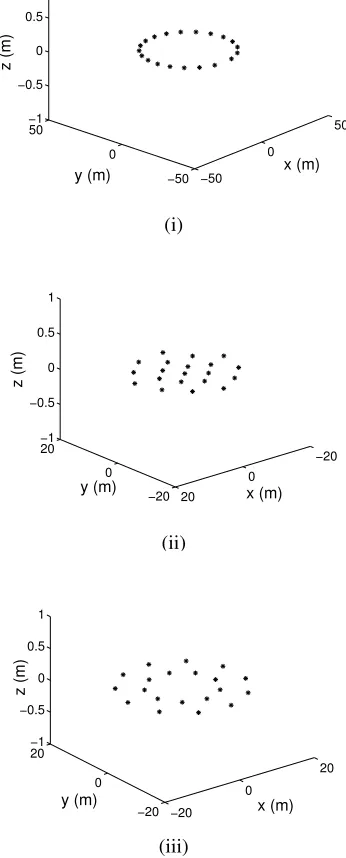
In order to test the control laws we consider a system of 20 spacecraft with mass 10 kg, required to form the three different formations; cluster, ring and double ring. Each spacecraft are given random initial positions on the x-y plane and an initial speed equal to0.1 ms−1. During the first time period (t= 0−8000s) the system of spacecraft are driven to a ring of diameter 50 m and then forced into a cluster state (t= 8000−16000 s) with diameter equal to 30 m. Once in this state a bifurcation is performed on the system and two rings are formed with the outer ring corresponding to a diameter of 30 m and an inner ring with diameter14 m (t= 16000−24000s). The results of the simulation are given in Fig. 6 with Table I noting the value of the parameters during each stage.

TABLE I

BOUND CONTROL FORMATION PATTERN CONSTANTS

Formation µ r Ch Ce Le Cz Cr Lr σ

Ring 0 25 0_.05 _{- -} 0_.01 1 1 0_.5

Cluster 0 0 0_.05 _{- -} 0_.01 1 2 2

Two rings 4 11 0.1 _{0.1 5} 0.01 1 2 5

B. Actuator Saturation

From Eq. 2 we can determine the control force acting on each spacecraft as shown in Eq. 34.

ui=uS+uR+ud (34)

where,





uS

uR

ud



=





−∇iUS(xi) −∇iUR(xij)

−σvi



 (35)

Through the triangle inequality [26] the maximum control force must be;

|ui|6|∇iUS(xi)|+|∇iUR(xij)|+|σvi| (36)

The maximum control force that the system is required to produce will therefore be dependent upon the sum of the

−50 0

50

−50 0

50 −1 −0.5 0 0.5 1

z (m)

y (m) x (m)

(i)

−20 0 20

−20 0

20 −1

−0.5 0 0.5 1

z (m)

x (m) y (m)

(ii)

−20 0

20

−20 0 20 −1 −0.5 0 0.5 1

x (m) y (m)

z (m)

[image:6.612.332.505.15.444.2]

(iii)

Fig. 6. Bound Control Pattern Transition: (i) ring (t= 8000s) (ii) cluster (t= 16000_{s) (iii) double ring (t}= 24000_s)

maximum gradient of the steering and repulsive potentials and the maximum speed that each spacecraft can move.

As the purpose of the new steering potential is to have a bound control force it is important to determine the maximum control force for the hyperbolic and exponential potential functions in order to place a bound on the steering potential. If we consider the hyperbolic function, the control force,uh, is shown in Eq. 37 and Fig. 7;

uh = −∇iUh(ρi, zi)

=

"

− Ch(ρi−r) [(ρi−r)2+ 1]0.5

,−_(z2Czzi

i + 1)0.5

#T

(37)

-1.5 -1 -0.5 0 0.5 1 1.5

0 2 4 6 8 10 12 14

ρi uh

Ch

-Ch

(i)

-1.2 -1 -0.8 -0.6 -0.4 -0.2 0

0 2 4 6 8 10 12 14

zi uz

-Cz

[image:7.612.75.249.10.259.2]

(ii)

Fig. 7. Hyperbolic Control Force: (i)ρidirection (Ch= 1) (ii)zidirection (Cz= 1)

and aszi→ ∞,uz→ −Cz as shown in Fig. 7.

If we now consider the exponential control force as shown in Eq. 38;

ue = −∇iUe(ρi, zi)

=

2µCe

Le(ρi−r) exp

−(ρi−r)2/Le_,0

T

(38)

The maximum exponential control forces occurs when

ρi=r±

q

Le

2 giving the maximum control force,ue, equal

to±√2µexp−0.5_√Ce

Le as shown in Fig. 8.

-1 -0.8 -0.6 -0.4 -0.2 0 0.2 0.4 0.6 0.8 1

0 2 4 6 8 10 12

ρi

ue

Ue maximum

[image:7.612.330.507.98.358.2]

Ue maximum

Fig. 8. Exponential Control Force (µ= 1_,Ce= 1_andLe= 1₎

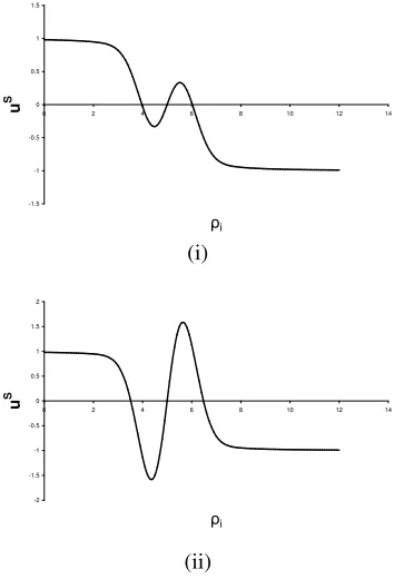
Therefore, depending upon the constants chosen in the equations the maximum bound control force in the ρi direction will either be controlled through the hyperbolic or exponential term in the steering potential equation. The equations have to be evaluated to determine if either the

hyperbolic or exponential term dominates as shown in Fig. 9 (i) and (ii). Considering the case whenµ >0with constants choosen so that the hyperbolic term dominates then, |∇iUS(ρi)|max = Ch. If, however, the exponential term dominates then|∇iUS_{(ρi)|maxcan be found numerically. In} the z direction,|∇iUS_(zi)|max=C

zas shown in Fig. 7 (ii).

-1.5 -1 -0.5 0 0.5 1 1.5

0 2 4 6 8 10 12 14

ρi

u

S

(i)

-2 -1.5 -1 -0.5 0 0.5 1 1.5 2

0 2 4 6 8 10 12 14

ρi

u

S

(ii)

Fig. 9. Steering Potential Control Force: (i) uh dominating (ii) ue dominating

The bound steering potential control force is then;

|uS_| = |∇iUS(xi)|max ≤ h ∇iUS_(ρi)max2

+ ∇iUS_(zi)max2i0.5

(39)

The repulsive potential is a bound force that has a maximum value equal to CR/LR that occurs when

xij = 0. This would, however, occur when two spacecraft are in the same position and therefore would have collided. The realistic maximum control force would therefore be (uR_i)max = CR/LRexp−(|xij|min/LR) where, |xij|min=|xi−xj|min, is the minimum separation distance between both spacecraft without colliding as shown in Fig. 10 (ii) for example.

The maximum control force is therefore;

|uR_|=|∇iUR(xij)|max=

Cr

Lr

exp−|xij|min/Lr ₍₄₀₎

where, |x_ij|min = Lrln

_2C

r

mV2

m

and Vm can assumed

[image:7.612.42.251.482.601.2]

0 0.2 0.4 0.6 0.8 1 1.2

0 1 2 3 4 5 6

|xij|

U

R

|xij|min

(i)

0 0.2 0.4 0.6 0.8 1 1.2

0 1 2 3 4 5 6

|xij|

u

R

ui

R max

[image:8.612.343.490.80.422.2]

(ii)

Fig. 10. Repulsive potential: (i) potential function (ii) control force

constantσis large as discussed insection II B.

The dissipative force,udis bound by the maximum speed,

Vm. Therefore;

|ud_|=|σvi|max≤σVm (41)

The maximum total force that the actuator will generate is therefore;

|ui|6|∇iUS(xi)|+|∇iUR(xij)|+|σvi| (42)

If the steering potential is dominated by the hyperbolic term, the maximum control force is;

|u_i| 6 _|∇iUS(xi)|+|∇iUR(xij)|+|σv_i|

6 q

C2

h+Cz2+

Cr

Lr

exp−|xij|min/Lr_+σV

m(43)

If, however, the steering potential is dominated by the exponential term,|∇iUS_{(xi)|will have to be evaluated with} |∇iUS_{(zi)max| = C}

z, |∇iUR(xij)| = _LCr_rexp−|xij|min/Lr and|σv_i|=σVm.

From the results it can be seen that the desired formations are formed during the simulation. From section II A

we know that the minimum separation distance between the spacecraft occurs when the spacecraft is traveling at its maximum speed equal to Lrln

2Cr

mV2 m

. During the formation of the first two stages the maximum bound control force acting is equal to that given in Eq. 43. Similarly in the formation of the double ring state when the steering potential is influenced by both the hyperbolic

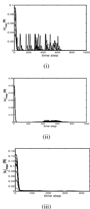
and exponential term, as the hyperbolic term dominates the maximum bound control force is also given by Eq. 43. The control force calculated from the simulation is given in Fig. 11 and summarised in Table II with a comparison to the upper bound estimated previously.

0 200 400 600 800 1000

0 0.02 0.04 0.06 0.08 0.1

time step |ui

|max

(N)

(i)

0 200 400 600 800 1000 0

0.01 0.02 0.03 0.04 0.05 0.06

time step |ui

|max

(N)

(ii)

0 100 200 300 400

0 0.02 0.04 0.06 0.08 0.1 0.12 0.14 0.16

time step

|ui |max

(N)

(iii)

Fig. 11. Numerical control force: (i) formation of ring (ii) formation of cluster (iii) formation of double ring

TABLE II

ANALYTICAL ANDCOMPUTATIONCONTROLFORCE

Formation Maximum Analytical Simulated Maximum Control Force (N) Control Force (N)

Ring 0.15 0.09

Cluster 0.27 0.05

Two rings 0.63 0.15

[image:8.612.314.523.501.554.2]

the maximum simulated control force during each formation is less than the maximum analytical bound control force. A real system could therefore be designed in such a way that the actuator saturation can be avoided so that the desired formation will form.

V. CONCLUSION

We have shown that the control of spacecraft flying in formation can be achieved through the use of the artificial potential function method. We have extended previous re-search in this area through the use of bifurcation theory to demonstrate that through a simple parameter change a for-mation of spacecraft can be made to alter their configuration. To ensure that desired behaviours always occur the stability of the system is proven mathematically through dynamical systems theory. In order to overcome the real problem of actuator saturation we have shown how a bound control force can be achieved through a hyperbolic/exponential function and demonstrated this for a system of20spacecraft of mass 10kg and maximum speed of 0.1ms−1. The control force achieved in simulation was found to be smaller than the analytical solution so that a real system could be designed in such a way that the real problem of actuator saturation can be avoided.

REFERENCES

[1] Roberts J. A.Satellite formation flying for an interferometry mission. PhD thesis, Cranfield University, 2005.

[2] Carpenter K. The stellar imager: a revolutionary large-baseline imaging interferometer at the sun-earth l2 point. InProceedings of the SPIE Conference on New Frontiers in Stellar Interferometry, Glasgow, June 25, 2004.

[3] Wallner O. Darwin system assessment study. Astrium Summary Report, Issue 1, pp. 1-30 (European Space Agency), 12 December, 2006.

[4] Scharf D.P., Ploen S.R., and Hadaegh F.Y. A survey of spacecraft formation flying guidance and control (part ii): Control. InAmerican Control Conference, Vol.4 p2976-2985, Colorado, June 4-6, 2003,. [5] Lawton J.R.T. A behavior-based approach to multiple spacecraft

formation flying. PhD thesis, Brigham Young University, 2000. [6] Scharf D.P., Hadaegh F.Y., and Ploen S.R. Precision formation

delta-v requirments for distributed platforms in earth orbit. Jet Propulsion Laboratory, National Aeronautics and Space Administration Technical Report, No. 13, November 9, 2004.

[7] Jones P.B., Blake M.A, and Archibald J.K. A real-time algorithm for task allocation. In International Symposium on Intelligent Control, p672-677, Vancouver, October 27-30, 2002.

[8] Ren W. and Beard R.W. A decentralized scheme for spacecraft formation flying via the virtual structure approach. In Proceedings of the American Control Conference, Colorado, June 4-6, 2003. [9] Do K.D. and Pan. J. Nonlinear formation control of unicycle-type

mobile robots.Robotics and Autonomous Systems, Vol. 55, No. 3:191– 204, March 2007.

[10] Wang P.K.C and Hadaegh F.Y. Coordination and control of multiple microspacecraft moving in formation. Journal of the Astronautical Sciences, Vol. 44, No. 3:315–355, 1996.

[11] Wong H. and Kapila V. Spacecraft formation flying near sun-earth l2lagrange point: Trajectory generation and adaptive output feedback control. InProceedings of the American Control Conference, p2411-2418, Portland, June 8-10, 2005.

[12] Bauer F., Bristow J., Folta D., Hartman K., Quinn D., and Howt J.P. Satellite formation flying using an innovative autonomous control system (autocon) environment. In AIAA Guidance, Navigation, and Control Conference, p657-666, New Orleans, August 11-13, 1997.

[13] Grøtli E.I.Modeling and Control of Formation Flying Satellites in 6 DOF. PhD thesis, Norwegian University of Science and Technology, 2005.

[14] C. R. McInnes. Autonomous ring formation for a planar constellation of satellites. Journal Guidance, Control and Dynamics, Vol. 18, No. 5:1215–1217, 1995.

[15] Reif J.H. and Wang H. Social potential fields: A distributed behavioral control for autonomous robots.Robots and Autonomous Systems, Vol. 27, No. 3:171–194, 1999.

[16] McQuade F, Ward R, and McInnes C.R. The autonomous configuration of satellite formations using generic potential functions. In Inter-national Symposium, Formation Flying, Missions and Technologies, Toulouse, October 29-31, 2002.

[17] A. Badawy and C.R. McInnes. On-orbit assembly using superquadric potential fields.Journal of Guidance, Control, and Dynamics, Vol. 31, No. 1:30–43, 2008.

[18] Izzo D. and Pettazi L. Autonomous and distributed motion planning for satellite swarm.Journal of Guidance, Control, and Dynamics, Vol. 30, No. 2:449–459, 2007.

[19] Winfield A, Harper C, and Nembrini J. Towards dependable swarms and a new discipline of swarm engineering. InSAB Swarm Robotics Workshop, Santa Monica, July 17, 2004.

[20] D’Orsogna M. R, Chuang Y. L, Bertozzi A. L, and Chayes S. The road to catastrophe: stability and collapse in2_{d driven particle systems.}

Physical Review Letters, Vol. 96, No. 10:14302–1, 2006.

[21] Bennet D.J. and McInnes C.R. Pattern transition in spacecraft formation flying via the artificial potential field method and bifurcation theory. In3rd International Symposium on Formation Flying, Missions and Technologies, Noordwijk, The Netherlands, April 23-25, 2008. [22] Kalman R. E. and Bertram R. E. Control system analysis and design

via the second method of lyapunov part i: Continuous systems.Trans. ASME, Vol. 82:371–393, 1960.

[23] Kalman R. E. and Bertram R. E. Control system analysis and design via the second method of lyapunov part ii: Discrete systems. Trans. ASME, Vol. 82:394–400, 1960.

[24] Jordon D.W. and Smith P.Nonlinear Ordinary Differential Equations: An Introduction to Dynamical Systems. Oxford University Press, p432, 1999.

[25] LaSalle J. P. The invariance principle in the theory of stability.Centre for Dynamical Systems, Brown University (NASA Technical Report), June 23, 1966.