1
Three-Dimensional Formation Flying
Using Bifurcating Potential Fields
Masayuki Suzuki1 and Kenji Uchiyama2 Nihon University, Chiba, 274-8501, Japan
and
Derek. J. Bennet 3 and Colin R. McInnes4 University of Strathclyde, Glasgow, G1 1XJ, UK
This paper describes the design of a three-dimensional formation flying guidance and control algorithm for a swarm of autonomous Unmanned Aerial Vehicles (UAVs), using the new approach of bifurcating artificial potential fields. We consider a decentralized control methodology that can create verifiable swarming patterns, which guarantee obstacle and vehicle collision avoidance. Based on a steering and repulsive potential field the algorithm supports flight that can transition between different formation patterns by way of a simple parameter change. The algorithm is applied to linear longitudinal and lateral models of a UAV. An experimental system to demonstrate formation flying is also developed to verify the validity of the proposed control system.
Nomenclature F = artificial potential function
FS = steering potential function FR = repulsive potential function
μ = bifurcation parameter
ρ = parameter of formation pattern
Ch = amplitude parameter of hyperbolic potential function
Cr = amplitude parameter of repulsive potential function
Lr = length parameter of repulsive potential function
Ce = amplitude parameter of exponential potential function
Le = length parameter of exponential potential function
r = UAV position vector
v = UAV velocity vector U = forward velocity V = side velocity W = vertical velocity
p = roll rate
q = pitch rate
r = yaw rate
φ = roll angle
θ = pitch angle
ψ = yaw angle
δe = elevator deflection from trim condition
δa = aileron deflection from trim condition
1
Graduate Student, Department of Aerospace Engineering, [email protected]. 2
Associate Professor, Department of Aerospace Engineering, [email protected], AIAA Senior Member.
3
Ph.D Student, Department of Mechanical Engineering, [email protected]. 4
δr = rudder deflection from trim condition
δt = thrust offset from trim condition
X, Y, Z = Forces of translational motion L, M, N = Moments of forces
Φ,Θ,Ψ = Euler angles
I. Introduction
NMANNED Aerial Vehicles (UAVs) have been applied to many applications such as scientific data gathering and reconnaissance for civil or military purposes. As the number of UAVs has increased decentralized control methods have been developed to overcome the complexity of a UAV system, as controlling the system in a centralized way becomes unrealistic. In the area of swarming systems some of the research is motivated by emergent and self-organizational behavior in nature. By using a concept of behavioral control architecture, taking inspiration from the natural world, we can design a control system that has the advantages of a being a scalable, robust, and flexible system.
U
Artificial potential fields are an example of a behavior based architecture applied to the design of controllers for swarming systems.1-7 The basic idea of the theory is to create a workspace where each UAV is attracted towards equilibrium states whose stability is generally guaranteed by the Lyapunov direct method. There is, however, a possibility that a control system becomes overly complex when the goal state varies during a mission.1 Bennet and McInnes have applied classical bifurcation theory to the potential field to overcome this problem.4, 5 The method, which is simple and fast to execute, can allow for different configurations to be formed through a simple parameter change of the potential function. In this paper, we expand the method so as to be able to form a three-dimensional flight configuration.
There has been considerable focus on theoretical studies in the area of multiple UAVs, 7-11 however, experimental results8 validating the design of a formation controller are still rare. In general, the workload required to maintain a formation and to complete any mission in real time will be proportional to the number of UAVs. The system must make progress towards a goal state while avoiding unexpected obstacles and vehicle collisions. Thus we have developed an experimental system for UAVs such that each is able to operate autonomously. The aim of this paper is to develop a control methodology for a mission such as three-dimensional formation flying of UAVs and to verify its validity through numerical simulation and experiments.
II. Formation Flying
[image:2.612.172.443.493.672.2]A. Guidance Law
Figure 1 shows inertial coordinate system o-xyz and position vectors of UAVs.
Figure 1. Definition of position vectors. ri
rj
rij
z
y o
ithUAV
jthUAV
We consider a swarm of homogeneous UAVs, which are treated as a particles, each of which interacts via an the velocity field vi(1 ≤ i ≤ n) using a steering potential F S and a repulsive potential F R governed by Eq. (1)
(1) ) r ( ) r (
vi =−∇iFS i −∇iFijR ij
The desired velocity acting on each UAV is defined inthe following equations.
( )
( )
c i ij R ij i i S i x u x x F x x F v + ∂ ∂ − ∂ ∂ − =, (2)
3
( )
( )
i ij ij i i i y y y F y y F v ∂ ∂ − ∂ ∂ − = , R S (3)where ucis the constant desired final speed.
The desired command speed and heading angle of each UAV are therefore 2
, 2
, ,i xi yi
d v v
v = + (4)
⎟ ⎟ ⎠ ⎜ ⎜ ⎝ = i x i y i d v v , , , arctan ⎞ ⎛
ψ
(5)The steering potential4F S is defined as shown in Eq. (6).
( )
(
)
(
)
⎟⎟ ⎠ ⎞ ⎜ ⎜ ⎝ ⎛− − + + − = e d i e d i h i S L C C F 2 2 exp1
μ
ρ
ρ
ρ
ρ
(6)where Chrepresents the amplitude of hyperbolic potential function, μ is the bifurcation parameter, Ce and Le
represent the amplitude and length scales, respectively, of the exponential potential function, ρis desired parameter of formation pattern and subscript d denotes desired value. We define ρi by the following equation
[ ]
T i i i =Tl,x′ρ
(7)where
2 2
i i
i x y
l = ′ + ′ ,
⎥ ⎥ ⎥ ⎦ ⎤ ⎢ ⎢ ⎢ ⎣ ⎡ = ⎥ ⎥ ⎥ ⎦ ⎤ ⎢ ⎢ ⎢ ⎣ ⎡ ′ ′ ′ i i i i i i z y x DCM z y x ⎥ ⎥ ⎥ ⎦ ⎤ ⎢ ⎢ ⎢ ⎣ ⎡ Θ Φ Ψ Φ − Ψ Θ Φ Ψ Φ + Ψ Θ Φ Θ Φ Ψ Φ − Ψ Θ Φ Ψ Φ − Ψ Θ Φ = cos cos ) cos sin sin sin (cos ) sin sin cos sin (cos cos sin ) cos cos sin sin (sin ) sin cos cos sin (sin DCM Θ − Ψ Θ Ψ
Θcos cos sin sin
cos
Three-dimensional formation flying can be achieved by manipulating the parameter matrixT
∈
R2and the Direction Cosine Matrix (DCM). If T is [1 0] the circle formation pattern is generated. In the case of [0 1] a straight formation pattern is generated .In addition we can change angle of the plane formation pattern formed using the Euler angles,Depending on the value of μ, the steering potential can change the number of stationary points and have various forms. Figures 2 and 3 show examples of the potential field when μ is negative and positive. In particular, the steering potential has one state of dynamical equilibrium at a desired distance r as shown in Figs. 2(a) and 3(a) when the parameter μ is negative. On the other hand, when μ is positive the steering potential has two stationary states as shown in Figs. 2(b) and 3(b). These results imply that the formation pattern can be changed easily through manipulation of the parameter μ , ρd, T, Φ, Θ and Ψ.
Stationary states Stationary state
[image:4.612.111.510.158.323.2](a) μ < 0 (b) μ > 0
Figure 2. Bifurcating potential field (T= [0 1], d =0, Ce=3, Le=3, Ch=3).
Figure 3. Bifurcating potential field (T= [1 0], , ρd =10, Ce=1.5, Le=5, Ch=0.2).
Stationary state
(b) μ > 0 Stationary states
(a) μ < 0
The repulsive potential12 is defined in the following equation
∑
≠ ⎟
⎟ ⎠ ⎞ ⎜ ⎜ ⎝ ⎛ − =
i j
j r
ij r
R ij
L C
F
,
exp r (8)
where Cr and Lr represent the amplitude and length scales of the repulsive potential function, respectively, and
| rij | = | ri – rj |. The total repulsive bound velocity on the ith UAV is dependent on the position of the other (n-1)
UAVs in the formation. The repulsive potential is therefore used to ensure that as the UAVs are steered towards the goal state they do not collide with each other.
[image:4.612.93.513.361.529.2]Lyapunov’s Second Theorem and an eigenvalue analysis of the linearized equations of motion.4,5 The results of this analysis indicate that the system can always be considered as stable.
B. Control Law
To achieve steady-state flight we use a robust controller for a linear time-invariant multi-variable system.13 We can express state and output equations for longitudinal and lateral motion which is linearized around the equilibrium point, as
5
) ( Bu ) ( Ax ) (
x& t = t + t (9)
) ( Cx ) (
y t = t (10)
Firstly we define the error e (t) between the output y and input yd as shown in Eq.(11) .
d
t) y y (
e = − (11)
We differentiate Eq. (9) obtaining
) ( ) ( )
(t t t
dt d
u B x A
x& = & + & (12)
Assuming yd=0, then
) ( x C ) (
et t
dt d
&
= (13)
Combining Eqs. (12) and (13) we have a system as follows;
) ( u 0 B ) ( e
) ( x 0 C
0 A ) ( e
) ( x
t t
t t
t dt
d
& &
&
⎥ ⎦ ⎤ ⎢ ⎣ ⎡ + ⎥ ⎦ ⎤ ⎢ ⎣ ⎡ ⎥ ⎦ ⎤ ⎢ ⎣ ⎡ = ⎥ ⎦ ⎤ ⎢ ⎣ ⎡
(14)
In order to make this system stable we should consider the rank of the following matrix derived from Eq. (14).
(15) p
n rank ⎥= +
⎦ ⎤ ⎢ ⎣ ⎡
0 C
B A
yd
+
-K
1B
+
+
K
2s
I
C
A
+
s I
+
uFi
x y
where n is the order of the matrix A and p is the number of outputs. Accordingly, we can control only two variables for both the longitudinal and lateral equations, and we choose U andθ for longitudinal motion, and φ and ψ for lateral motion to control speed and attitude. The input for longitudinal and lateral motions of this controller u is given by Eq. (16)
(16)
∫
− −
= t t t dt
t
0 2
1 ( ) ( )
)
( K x K e
u
where K1 and K2 are the feedback gains of this controller.
The system we developed to achieve formation flying is summarized in Fig.5.
III. Numerical Simulation
A. UAV Dynamics
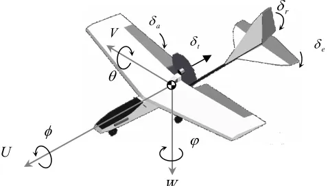
To simulate swarm control of the UAVs, we used a model14 for the UAV that is linearized about straight and level flight conditions with a forward speed of 12.5m/s and θ 0=-0.447deg. Figure 6 shows the definition of the state variables and control inputs.
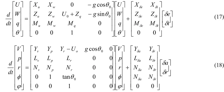
⎥ ⎦ ⎤ ⎢ ⎣ ⎡ ⎥ ⎥ ⎥ ⎥ ⎦ ⎤ ⎢ ⎢ ⎢ ⎢ ⎣ ⎡ + ⎥ ⎥ ⎥ ⎥ ⎦ ⎤ ⎢ ⎢ ⎢ ⎢ ⎣ ⎡ ⎥ ⎥ ⎥ ⎥ ⎦ ⎤ ⎢ ⎢ ⎢ ⎢ ⎣ ⎡ − + − = ⎥ ⎥ ⎥ ⎥ ⎦ ⎤ ⎢ ⎢ ⎢ ⎢ ⎣ ⎡ t e M M Z Z X X q W U M M M g Z U Z Z g X X q W U dt d t e t e t e q w u q w u w u
δ
δ
θ
θ
θ
θ
δ δ δ δ δ δ 0 0 0 1 0 0 0 sin cos 0 0 0 0 (17) ⎥ ⎦ ⎤ ⎢ ⎣ ⎡ ⎥ ⎥ ⎥ ⎥ ⎥ ⎥ ⎦ ⎢ ⎢ ⎢ ⎢ ⎢ ⎢ ⎣ + ⎥ ⎥ ⎥ ⎥ ⎥ ⎥ ⎦ ⎢ ⎢ ⎢ ⎢ ⎢ ⎢ ⎣ ⎥ ⎥ ⎥ ⎥ ⎥ ⎥ ⎦ ⎢ ⎢ ⎢ ⎢ ⎢ ⎢ ⎣ = ⎥ ⎥ ⎥ ⎥ ⎥ ⎥ ⎦ ⎢ ⎢ ⎢ ⎢ ⎢ ⎢ ⎣ r a N N N N L L r p N N N L L L r p dt d r a r a r a r a r p v r p v o r p vδ
δ
ϕ
φ
θ
ϕ
φ
δ δδ δ δ δ δ δ 0 0 0 0 1 0 0 0 0 tan 1 0 0 0 0 0 0
0 ⎤⎡ ⎤ ⎡ ⎤
⎡ −
⎤
⎡V Y Y Y U gcos
θ
0 V Y Y(18)
where U, V, W, p, q, r, φ, θ, ψ are variables and, δt, δa, δr, δe are deflections of moving surfaces from trim conditions. Tables 1 and 2 show the linearized parameters of longitudinal and lateral motions, respectively. Subscripts denote partial derivatives respect to the parameters.
+
φdθd
ψd
Ud
Guidance Law Control Law ith
UAV xj yj zj δe δt δa δr φ θ ψ U xi yi zi
jth UAVs
[image:6.612.151.540.446.606.2]μ , T, ρd
r
δ
aδ
V
t δ
e δ
7
B. Simulation Results
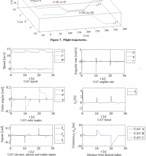
A numerical simulation was performed to verify the proposed control law. We were able to generate different formations, such as a ring or a cluster by using the potential functions. The ring formation places UAVs on a circle. They can be formed on concentric circles with different radii by changing parameters in the hyperbolic potential function. The cluster formation closes up UAVs equally with distances determined by parameters of the repulsive potential function.
Figure 7 shows the transition of a formation of 3 UAVs flying with no wind. The simulation parameters are set to μ=0, T= [1 0], Φ=0, Θ=0, Ψ=0, Cr=2, Lr=2, Ch=2. Poles of the controller are placed at -10. The formation pattern
changed from a small ring (ρd=5) to a cluster (ρd=0) to a large ring (ρd=20). As can be seen from the values of the
desired radius in Fig.8, the system changes from a small ring to a cluster to a large ring every 10 s and we can see that each UAV attained desired radius. This is achieved through a simple parameter change and is one of the advantages of using a bifurcation equation as the basis for the artificial potential functions, as we do not need to control each UAV individually. The other parts of Fig.8 show the UAVs speed, angular velocity, Euler angles and the control inputs. The saturation limits for the aircraft control surfaces are δe= ±0.35rad and δa, δr = ±0.79rad, thrust is−0.35<δt<5.45N and we can see that the controller is within its limits.
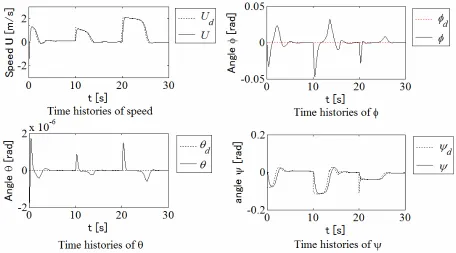
Figure 9 shows the time responses of the controlled variables of the UAV. From the results, it can be seen that each variable followed the commands satisfactory.
θ
φ
ϕ
U
[image:7.612.179.418.76.212.2]W
[image:7.612.104.513.254.449.2]Figure 6. Definitions of state variables and control inputs.
Table 2. Linearized parameters for lateral motion.
YU [s-1] -0.68
Yp [m s-1] -0.11
Yr [m s-1] -12.20
LV [m-1 s-1] -32.17
Lp [s-1] -56.38
Lr [s-1] 19.30
NV [m-1 s-1] 7.89
Np [s-1] -3.13
Nr [s-1] -4.00
Yδa [m s-2] -3.34
Yδr [m s-2] 22.99
Lδa [s-2] -26.88
Lδr [s-2] -6.80
Nδa [s-2] 58.46
Nδt [kg-1 m-1] -226.79
Table 1. Linearized parameters for longitudinal motion.
XU [s-1] -0.13
XW [s-1] 0.14
ZU [s-1] -3.17
ZW [s-1] -13.06
Zq [m s-1] 1.37
Uo [m] 12.5
MU [m-1 s-1] -1.95
MW [m-1 s-1] -17.41
Mq [s-1] -21.86
Xδe [m s-2] 0
Xδ t [kg-1] 2.32
Zδe [m s-2] -7.73
Zδ t [kg-1] 0
Mδe [s-2] -205.25
Mδt [s-2] 0
[image:7.612.323.506.262.446.2]Figure 7. Flight trajectories.
t=10, ρd=0
t=20, ρd=20
t=30 t=0,ρd=5
Figure 9. Time histories of speed and Euler angles(UAV A).
9 IV. Experiment
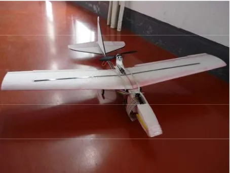
We developed an experimental system for formation flying of multiple UAVs to test the validity of the proposed formation controller. Each UAV, which is controlled by a throttle and control surfaces, the elevator, the ailerons, and rudder, needs absolute position, attitude, altitude and ground speed for formation flying using the law described in the preceding chapter. The avionics consists of a GPS module, which provides the ground speed, altitude and heading angle, a microcomputer, which controls a UAV autonomously, and an inertial measurement unit (IMU), which measures accelerations along 3axes and angular rates around 2axes. Attitude angles can be solved for using the measured acceleration. The system configuration for autonomous flying is illustrated in Fig.10. In order to cope with the emergency of a system malfunction during automatic control, a radio control transmitter can also operate the UAV. Figure 11 shows the method of communication between UAVs and a ground station. A ground station sends guidance commands U, φ, θ andψ to each UAV. Each UAV transmits its position to the ground station. We developed the UAVs as shown in Figs. 12 and 13.
Tables 3 to 6 show the specification of the avionics built into the UAV. Table 7 describes the specification of the UAV.
Ground station UAV A UAV B UAV C
Radio
communication
Figure 11. Overview of experimental system.
CPU
GPS receiver Radio
Radio Ground station UAV
Radio control transmitter Radio control receiver DC motor
DC servomotor×3 Three axis accelerometer
Switch
serial servo pulse 2.4GHz
analog
[image:9.612.349.516.541.681.2]Two axis angular rate sensor
Table 3. Microcomputer(SH7145F).
CPU HD64F7145F50 Operation clock [MHz] 49.152
SCI×4ch 10bit A/D converter×8ch Functions
16bit timer
Table 4. IMU (IDG-300).
Acceleration [g] -3~3
Sensitivity [mV/g] 300
Angular rate [deg/s] -500~500 Sensitivity [mV/deg/s] 2.0
Table 5. Radio communication module (MU-2-429).
V. Conclusion
In this paper, we have described how a guidance law with an artificial potential field and bifurcation theory can change formation patterns easily with a simple parameter change and we have extended this law to three-dimensional formation flying. The numerical results showed that a guidance law based on the potential function is a viable method to control formation flying of UAVs. We developed a UAV that has an inertial navigation system and a global positioning system. The UAV satisfied the specifications required to perform experiments in formation flying. A flight-testing program using the experimental system will be demonstrated to verify the proposed controller.
Acknowledgement
This work is supported by Japan Society for the Promotion of Science (No. 21560822). Reference
1
Shimada Y., Uchiyama K., et al, “Proximity Maneuver and Obstacle Avoidance Control Using Potential Function Guidance Method,” Proceedings of International Symposium on Space Technology and Science, 2006, pp.557-562
2
McInnes, C. R., “Potential Function Methods for Autonomous Spacecraft Guidance and Control,” Adv Astronaut Sci, Vol.90, No.Pt2, 1996, pp.2093-2109.
3 McInnes C. R., “Velocity field path-planning for single and multiple unmanned aerial vehicles, The Aeronautical
Journal, Vol. 107, No.1073, 2003, pp. 419-426.
Compatible specification ARIB STD- 67 Frequency range [MHz] 429.250 429.7375
Number of channels 40
Power [mW] 10
Modulation 2FSK,4,800bps
Table 6. GPS module (EB-85A).
Update rate [Hz] 5 Sensitivity [dBm] -158 Positional accuracy [m] 2.6
Table 7. Specification of UAV (Savanna).
Length [mm] 890
Span [mm] 930
Weight [g] 290
[image:10.612.71.298.89.260.2]Material Expanded polypropylene
Figure 12. Overview of developed UAV.
Radio
communication module
CPU Radio control receiver
IMU GPS
[image:10.612.71.545.108.485.2]module
[image:10.612.265.536.261.476.2] [image:10.612.73.302.285.460.2]11 4
Bennet D. and McInnes C. R., “SpaceCraft Formation Flying Using Bifurcating Potential Fields, International Astronautical Congress, IAC-08-C1.6.4, 2008.
5
Bennet D. and McInnes C. R., “Pattern Transition in SpaceCraft Formation Flying via The Artificial Potential Field Method and Bifurcation Theory,” 3rd International Symposium on Formation Flying, Missions and Technologies, 2008.
6
Huang W. H., Fajen B. R., Fink J. R., and Warren W. H., “Visual Navigation and Obstacle Avoidance Using a Steering Potential Function,” Robotics and Autonomous Systems, 54, 2006, pp.288-299
7
Paul T., Krogstad T. R., and Gravdahl J. T., ”Modeling of UAV Formation Flight Using 3D Potential Field,” Simulation Modeling Practice and Theory, Vol.16, Issue 9, 2008, pp.1453-1462.
8
Gu. Y. et al., “Design of Flight Testing Evaluation of Formation Control Laws”, IEEE Transaction on Control Systems Technology, Vol.14, No.6, 2006, pp.1105- 1112.
9
Ryoo C. K., Kim Y. H., and Tahk M. J., “Optimal UAV Formation Guidance Laws with Timing Constraint,” International Journal of Systems Science, Vol.37, No.6, 2006, pp.415 – 427.
10
Kim S. and Kim Y. , “Three Dimensional Optimum Controller for Multiple UAV Formation Flight Using Behavior-based Decentralized Approach,” International Conference on Control, Automation and Systems, 2007, pp.1387-1392.
11
Lee J. et al. “Formation Geometry Center based Formation Controller Design using Lyapunov Stability Theorem,” 2008 KSAS-JSASS Joint International Symposium, 2008, pp.614-618.
12
D'Orsogna M. R., Chuang Y. L., Bertozzi A. L., and Chayes L. S., “The Road to Catastrophe: Stability and Collapse in 2D Driven Particle Systems,” Physical Review Letters, Vol.96, No.10:14302-1, 2006.
13
Davison E. , “The robust control of a servomechanism problem for lineartime-invariant multivariable systems.” Automatic Control, IEEE Transactions on, 21(1), 1976, pp. 25–34.
14

![Figure 2. Bifurcating potential field (T= [0 1], d =0, Ce=3, Le=3, Ch=3).](https://thumb-us.123doks.com/thumbv2/123dok_us/1705990.123976/4.612.93.513.361.529/figure-bifurcating-potential-field-t-ce-le-ch.webp)