A GEANT4 simulation of the SAGE spectrometer and its first application to 255Lr

(1)

A GEANT4 Simulation of the SAGE

Spectrometer and its First Application to

255 Lr

Thesis submitted in accordance with the requirements of the University of Liverpool for the degree of Doctor in Philosophy

by

Daniel Martin Cox

(2)

Abstract

A two-part experiment studying 255Lr was performed in the University of Jyv¨askly¨a, Finland. The nucleus was created in the fusion-evaporation re-action 209_Bi(48_Ca,2n)255_{Lr. The first part was performed using RITU and}

GREAT, and was run at a high intensity to study the decay properties of

255_{Lr. The second part combined RITU, GREAT, and SAGE, and was run}

at a lower intensity to study excited states in 255_Lr.

In parallel a comprehensive GEANT4 simulation has for the SAGE spec-trometer has been developed. With the goals of better characterising the experimental setup, and allowing the simulation of complex level schemes such as those seen in255Lr for the purposes of testing proposed level schemes by direct comparison to experimental data.

(3)

“A university is very much like a coral reef. It provides calm waters and food particles for delicate yet marvellously constructed organisms that could not possibly survive in the pounding surf of reality, where people ask questions like ‘Is what you do of any use?’ and other nonsense.”

Science of Discworld

(4)

Acknowledgements

First and foremost I would like to thank my supervisor Prof. Rodi Herzberg for all his guidance and support during my PhD.

I am incredibly grateful to Philippos for the endless advice and patience over the last four years.

A big thank you to everyone at the University of Jyv¨askyl¨a for all their help and support over the years and to all the people that brightened up my time there on experiments, far too many to name them all here, but especially all the past and present members of Team Herzberg, Philippos, Andy, Andrew, Fuad, and Eddie.

Thanks to all the students and postdocs in the Department for all the good times over the years, the conferences, the summer school, the beers, the incredibly varied and often surreal lunchtime conversations. It was never dull. Thanks must go to Pete, Joe, and Pete, for always patiently listening to my demented GEANT4 based ravings over the years. Special mention goes to my year mates, Mark, Joe, Pete, Anthony, and Baha for being there through it all, the highs and the lows.

My sincere gratitude goes to, again, Dr Philippos Papadakis and Dr Gemma Wilson for their skills as proof readers of this work. Without them, it wouldn’t make much sense.

I would also like to acknowledge the STFC, for providing the necessary financial support for this research project.

(5)

List of Figures

1.1 Self-consistent mean-field calculations for shell correction

ener-gies, in MeV,for the Z∼50 region, and the super heavy nuclei[Ben01]. 3 2.1 A plot of binding energy per nucleon as a function of mass

number [Cas01]. . . 8 2.2 Chart of nuclides overlaid with the predicted binding energy

per nucleon according to the liquid drop model, also line for various values ofZ2_/A _{tracking the fissility [Sch13]. . . .} ₁₁

2.3 Schematic representation of angular momentum coupling of a prolate nucleus with a single particle orbiting. . . 14 2.4 Illustration of different types of isomers taken from [Wal99]. . 17 2.5 A section of Segr´e chart, showing the longest lived isomers

Z≥82 [Her11]. . . 18 2.6 Internal conversion coefficients αk and αtot, as a function of

energy for E2 and M1 transitions in lawrencium. . . 27

3.1 Schematic Diagram of the setup at Jyv¨askyl¨a, showing JU-ROGAM II and the SAGE silicon detector along with RITU and GREAT [Pap09]. . . 29 3.2 The JUROGAM II array, purple dewars indicate Clover

detec-tors, the golden dewars, Phase I’s. At the front the hexagonal gap can be seen where the 5 Phase I detectors have been re-moved to make space for the solenoidal magnet. . . 29 3.3 Schematic drawing of the SAGE silicon detector showing the

arrangement of the pixels. . . 30 3.4 Schematic of the RITU gas filled separator. . . 31 3.5 Schematic of the GREAT Focal Plane Array [Pag03]. . . 33 3.6 Efficiency curve for various components in the GREAT focal

plane array - obtained from [GJ08]. . . 35

(8)

4.2 Cross section view of two Clover(centre, right) and one Phase I (left) Ge detectors. . . 39 4.3 Comparison of simulated and real Si detectors. . . 39 4.4 Comparison of simulated and real high voltage barriers, note

the horseshoe is not shown in real image. . . 40 4.5 Schematic view of the magnetic coils and shielding within SAGE. 43 4.6 Comparison of electron distribution for original detector

po-sition (left) and detector moved by 10 mm towards the beam axis (right). . . 43 4.7 Simulated electrons in the SAGE silicon detector with an

ini-tial energy of 100 keV. . . 46 4.8 Simulated efficiency curve for the SAGE silicon detector

com-pared to measured values for peaks in 133_{Ba and} 207_Bi. _{. . . .} ₄₇

4.9 Simulated SAGE silicon detector efficiency as a function of high-voltage barrier setting. . . 48 4.10 Comparison of measured and simulated SAGE silicon detector

efficiency for a high voltage barrier setting of -30kV. . . 49 4.11 Simulated efficiency of the Jurogam II array also shown in blue

is a calculated efficiency curve. . . 50 4.12 Simulation detailing the geometry near to the target position

in SAGE, visible are the carbon foil unit, target wheel, target, and the detector chamber. . . 51 4.13 Detection efficiency as a function of distance downstream of

the target position for emission of electrons of energy 100 keV. 53 4.14 Electrons detected as a function of emission angle. . . 54 4.15 An example rotational band to be simulated. . . 58 4.16 Upper:γ-ray spectrum, lower:electron spectrum produced by

simulation of 1 million decays of level structure shown in Fig-ure 4.15. . . 59 4.17 An example strongly coupled rotational band to be simulated. 60 4.18 Upper γ-ray spectrum, lower electron spectrum produced by

simulation of 1 million decays of level structure shown in Fig-ure 4.17 with low intensity M1 transitions. . . 61 4.19 Upper γ-ray spectrum, lower electron spectrum produced by

simulation of 1 million decays of level structure shown in Fig-ure 4.17 with high intensity M1 transitions. . . 61

5.1 Relative efficiency curve for the SAGE silicon detector as a function of electron energy. . . 68 5.2 Absolute efficiency curve for the JUROGAM II array as a

(9)

6.1 Level scheme taken from [Jep09]. . . 76 6.2 Alpha decay scheme taken from Chatillonet al. [Cha06] . . . 77 6.3 γ-ray spectra taken from Ketelhut et al. [Ket09], (a) Singles

spectrum in delayed coincidence with recoil implantation (b)

γ −γ projection in coincidence with the sum of the gates of the transitions marked by dotted lines (c) same as (b) but for transitions marked with dashed lines. . . 77 6.4 An α spectrum of 255_{Lr, vetoed with the MWPC, visible are}

two peaks from255Lr, along with the αdecay daughter,251Md and contamination from 255_No. _{. . . .} ₇₉

6.5 A recoil-decay correlatedα-decay spectrum of255_{Lr, requiring}

the detection of a recoil nucleus in the 100 s prior to the α

detection. Peaks from the daughter nucleus 251_{Md and}

con-taminant 255_{No are also seen.} _{. . . .} ₇₉

6.6 Upper, recoil-αcorrelated spectrum of255Lr with a correlation time of 100 s, lower recoil-α-αcorrelated spectrum showing the daughter 251_{Md with a correlation time of 900 s. . . .} ₈₀

6.7 Two recoil-α−α correlated spectra inset with gating condi-tions on the α energy from the mother nucleus. . . 80 6.8 Decay curve for correlatedαdecays in 31 s half-life peak. Inset

shows the gating conditions with respect to α-particle energy. 82 6.9 Decay curve for correlatedα decays in 2.5 s peak. Inset shows

the gating conditions with respect toα-particle energy. . . 83 6.10 Decay curve for correlated isomeric decays, the short half-life

component is due to contamination from 206_{Pb. . . .} ₈₄

6.11 Recoil-electron tagged γ-ray spectrum from the focal plane Clover detectors. . . 85 6.12 Recoil-electron tagged γ-ray spectrum from the focal plane

planar detector, peaks marked with an * are known lawren-cium X-rays. . . 86 6.13 αdecay curve for correlatedαdecay in longer lived peak, inset

shows gating conditions. . . 88 6.14 Recoil-gated γ-ray spectrum from the JUROGAM II array.

Black labels indicate transitions in rotational band, red and blue indicate the two signature partner bands in the strongly coupled band. . . 90 6.15 Recoil-gatedγγcoincidence spectra, gating on a) knownγrays

(10)

6.16 Recoil-gated conversion electron spectrum from the SAGE sil-icon detector, a number of prominent peaks are labelled, en-ergies are uncorrected for binding energy. . . 92 6.17 Recoil-α-gated conversion electron spectrum from the SAGE

silicon detector, a number of prominent peaks are labelled, energies are uncorrected for binding energy. . . 93 6.18 Recoil-gatedγ-electron coincidence spectra, gating on a) known

γ rays in the rotational band b) knownγ rays in first signature partner band c) knownγ rays in second signature partner band. 94 6.19 Recoil-gated γ-ray spectrum gating on electrons at (upper)

50 keV, (middle) 64 keV, and (lower) 112 keV transitions. Shown in black, blue, and red, are the transitions in the rotational band, first signature partner and second signature partner bands, respectively. . . 95 6.20 Recoil-gated γ-ray spectrum gating on electrons at (upper)

76 keV, (middle) 104 keV, and (lower) 138 keV transitions Shown in black, blue, and red, are the transitions in the rotational band, first signature partner and second signature partner bands, respectively. . . 96 6.21 Recoil-gated γ-ray spectrum gating on electrons at (upper)

156 keV, and (lower) 188 keV transitions Shown in black, blue, and red, are the transitions in the rotational band, first signa-ture partner and second signasigna-ture partner bands, respectively. 97 6.22 Previously known bands from [Ket09]. . . 99 6.23 Kinematic moment of inertia for different values of spin of

lowest known level in 1/2− band. . . 100 6.24 Comparison of kinematic moment of inertia for different values

of spin of the lowest known level in the 1/2−band of255_{Lr with} 179_{Os and}181_{Pt. . . 101}

6.25 Comparison of the kinematic and dynamic moments of inertia for 255_{Lr and}179_{Os for excited states built upon the 1/2}− _state.102

6.26 Kinematic moment of inertia for different values of spin of lowest known level in the 7/2−band, also shown is the dynamic moment of inertia for comparison purposes. . . 103 6.27 Comparison of the kinematic and dynamic moments of inertia

for 255Lr and181Pt for excited states built upon the 7/2− state. 104 6.28 Proposed additional transitions based upon in-beam data and

(11)

6.29 Proposed level scheme for 255_{Lr broken down in the separate}

sections to be simulated. . . 106 6.30 Level scheme of 255_{Lr to be simulated in GEANT4, including}

all energies of M1 transitions, energies are in keV. . . 107 6.31 Possible structures built on various states in251Md[Cha07]. . . 111 6.32 1 million event simulation of rotational band built upon the

1/2− configuration from 255_{Lr. . . 112}

6.33 1 million event simulation of coupled band from 255Lr taking M1/E2 ratios for 7/2− configuration. . . 113 6.34 1 million event simulation of coupled band from 255_{Lr taking}

M1/E2 ratios for 7/2+ configuration. . . 114 6.35 Combined simulated spectra for decay of 255_{Lr. . . 115}

6.36 Comparison of simulated and measured 255_{Lr-tagged electron}

spectra for 255Lr Left axis shows experimental values, right simulated. . . 116 6.37 Comparison of simulated and measured electron spectra for

255_{Lr Left axis shows experimental values, right simulated. . . 117}

(12)

List of Tables

2.1 Transition probabilities T (s−1_{) for Weisskopf single particle}

estimates expressed asB(EL) andB(ML). The energiesE are measured in MeV [Rin04] . . . 24 2.2 Table of atomic electron binding energies for the innermost

transitions in lawrencium [Fir99] . . . 25

4.1 Number of electrons from one million generated at 100 keV interacting with different parts of the geometry, rounded to the nearest thousand. For the detector, only full energy deposits are considered, for all other volumes any energy deposit is counted. Note that an electron can deposit energy in multiple elements. . . 52 4.2 Example of level scheme file used for generation of radioactive

decays. L and G denote whether an entry is for a level or a γ

ray, respectively. . . 62 4.3 Example of one transition in an ICC file used for generation

of radioactive decays (E=40 keV, Z=103) . . . 63 4.4 Example of Intensity file used for generation of radioactive

decays. . . 63

5.1 Coefficients used for the fitting of the efficiency curve shown in Equation 5.1.2. Parameter denoted by * was held constant . 69

6.1 Experiment details. . . 75 6.2 Comparison of experimental details between Jeppesen et al.

(13)

Chapter 1 Introduction

One of the major questions in nuclear physics has always been what is the

limit of nuclear binding and to that end what is the heaviest nuclei that can

exist. The study of superheavy nuclei, those at the higher extremes of mass

and proton number, is at the forefront of this research as it is an excellent

testing ground for nuclear models. The nucleus is made up of positively

charged protons and uncharged neutrons held together by the strong force.

As the number of protons increases, so does the Coulomb repulsion that they experience. According to the liquid drop model (LDM) [Boh37] Coulomb

repulsion should become large enough to tear the nucleus apart for more

than 104 protons [Kru00], clearly this is not the case however. Elements

with Z up to 118 have been produced with relatively long half-lives [Oga07].

There must be other factors contributing to the binding of the nucleus.

The LDM was the first model to accurately describe nuclear properties

(14)

of protons and neutrons. From this came the idea that the nucleons had

specific arrangements in the nucleus, much like atomic electrons, and from

this arose the shell model.

There is a vast amount of experimental evidence for the existence of magic

numbers at 2, 8, 20, 28, 50, 82, for protons and neutrons, and also 126 for only neutrons [Cas01]. Furthermore, the next magic number, its value and its

very existence are greatly debated. Comparison of experimental observations

with theoretical models is vital to answering questions such as where is the

next island of stability? What is the heaviest bound nucleus that can exist?

According to theoretical predictions it is expected that a doubly magic

superheavy nucleus will have enhanced stability [Nil68, Nil69, ´Cwi05]. This

should lead to a so-called ”island of stability” [Sto06, Oga00] though the

limits of this are unknown.

The upper panel of Figure 1.1 shows theoretical shell closures for Z=50

nuclei. There is little variation within the models shown, and they all strongly

agree on Z=50 and N=82 being the most strongly bound. In the lower half

of this plot, however, there appears to be no definite closed shell but more

an area of increased stability centred between Z=114 and Z=126 depending

on the model.

Theoretical models can be split into two categories, microscopic-macroscopic models and self-consistent mean-field models. The former consist of a smoothly

varying component described by the LDM, and an oscillatory component

described by the shell model. The latter are formed by an iterative

proce-dure where an initial guess of the wavefunction is chosen to calculate the

(15)

un-Figure 1.1: Self-consistent mean-field calculations for shell correction ener-gies, in MeV,for the Z∼50 region, and the super heavy nuclei[Ben01]. til self-consistent convergance is achieved, and entirely shell model based.

Microscopic-macroscopic models generally predict the next doubly magic

nu-cleus to have Z=114 and N=184 [Nil68, Nil69, Par05, Par04, M¨ol94, M¨ol92]. Self-consistent models, however, generally disagree with the

microscopic-macroscopic predictions. Comparisons of the mean-field calculations [Kru00,

Ben01] indicate that non-relativistic models [ ´Cwi96, Ben99] give Z=124-126

and N=184. Relativistic models [Afa03, Ben03, Lal96, Ben99] predict a

higher Z=120 and a lower N=172. A detailed review of experimental studies

relevant to these calculations can be found in [Her11].

[image:15.595.163.438.131.396.2]

(16)

cross section for production of these elements is so low, that one event may

be detected in a day, a week, or even longer. With the heaviest studied so

far being 294

176118 [Oga06]. Here only 3 decay chains were detected in over

45 days of experiment. These extremely low production cross sections for

superheavy nuclei, <1 pb for element 118 [Arm03] mean that is not possible to get spectroscopic information. The heaviest nucleus to have any

spectro-scopic information measured is288_{115 [Rud13]. As can be seen in Figure A.1,}

some states that are involved in the closed shell at Z=114, drop in energy

with increasing deformation. Owing to this, these states are accessible in

excitations of lighter deformed nuclei in the Z∼102 region. These nuclei are relatively easy to produce in fusion evaporation reactions with cross sections

in the microbarn to nanobarn region. This allows for detailed spectroscopic

analysis, which can then be used to inform the theory of heavier spherical nuclei.

In-beam spectroscopic studies in γ-rays and conversion-electrons being

studied independently have lead to important insight into information such

as rotational structure, deformation and stability against fission. Even-even

nuclei such as 254No [Her02, Her06] and 250Fm [Gre08, Ros09, Bas06] have

been separately studied in both γ-ray and conversion-electron detection

ex-periments. Odd-mass nuclei do provide a more sensitive probe into single-particle structure at the cost of increased complexity, especially when studied

independently with γ-rays or conversion-electrons. Odd-mass nuclei 253_No

[Rei04, Rei05, Moo07], 251_{Md [Cha07],} 255_{Lr [Ket09] have been studied in} γ-ray, with 253_{No also being studied in conversion electrons [Her02, Her09].}

(17)

transitions has been established. The M1 transitions were not observed in

the early γ-ray experiments [Rei05, Rei04] owing to their low energy and

high conversion coefficients but were observed in the following conversion

electron study [Her02, Her09]. Later, in higher intensity γ-ray studies, some

of these M1 transitions were seen, but lower energy transitions still remain undetected. This case is similar to that of 255_{Lr, where alongside the ground}

state rotational band, a strongly coupled rotational band band has been

detected [Ket09]. The statistics were not high enough here to measure any

M1 transitions.

In this case a combinedγ-ray and conversion electron study of 255_{Lr has}

a higher sensitivity to these highly converted low-energy transitions whilst

retaining the ability to observe the higher energy known transitions, though

the cross section to produce 255Lr is very close to the current experimental limit with the lowest cross section studied in-beam being 60 nb for 256_Rf

[Rub13]. With that in mind it was decided that to meaningfully interpret

the results it was required to better understand the experimental response.

To that end a comprehensive GEANT4 simulation has been developed with

the aim of reproducing experimental data for purposes of testing proposed

level schemes and comparing to experimental data.

In this study, after an overview of the relevant theoretical framework, an experiment with the aim of studying excited states in255_{Lr will be presented.}

The experiment was performed at the University of Jyv¨askyl¨a using the

re-action209_Bi(48_Ca,2n)255_{Lr in two parts with a high intensity decay study at a}

(18)

Alongside this a comprehensive simulation package has been developed using

the GEANT4 toolkit [Ago03]. This simulation has been designed to include

all relevant geometries for the emission, tracking and subsequent detection

of γ-rays and conversion-electrons within the SAGE spectrometer. Within

this simulation there is the ability to enter possible structures and decays and reproduce the experimental response for that decay, which can then be

directly compared to the experimentally acquired data. Finally results of

(19)

Chapter 2 Theoretical Framework

2.1 Liquid Drop Model

The LDM was one of the first models proposed to explain the properties of the nucleus [Boh37]. The LDM treats the nucleus as an incompressible liquid

drop. This model successfully describes bulk properties of the nucleus, such

as fission, fusion, and α decay. However it fails to explain the experimental

observations of systematic deviations in properties such as binding energy,

nuclear charge radii, and the energy of the first excited state. It also fails to

explain to stability of superheavy nuclei since according to the liquid drop

model, nuclei with Z≥104 would be unbound. This led to the development of the shell model [GM49].

2.1.1 Binding Energy

The binding energy, B, of a nucleus is defined as the energy required to

(20)

nucleus is lower than the mass of its constituent particles byB/c2 _{which then}

follows that

B(Z, A) = Zmp+N mn−M(Z, A)

c2, (2.1)

from [Boh98], where mp and mn are the masses of the proton and neutron,

[image:20.595.156.445.255.495.2]

and M(Z,A) is the observed mass in the ground state.

Figure 2.1: A plot of binding energy per nucleon as a function of mass number [Cas01].

Binding energy is most often described in the form of binding energy per

nucleon, as shown in Figure 2.1, where binding energy per nucleon is plotted

as a function of mass number. There are a number of interesting conclusions

that can be drawn from this plot. The binding energy per nucleon increases

quickly untilA∼10, then there is a slower increase to A∼60, above thisB/A

(21)

attractive force experienced by each nucleon in the nucleus, B would increase proportionally with A2_{. This is not the case however, as B/A saturates at}

a maximum of just over 8 MeV. This indicates that each nucleon only feels

an attractive force from its nearest neighbours. From this it follows that

the nuclear force is a short range force. The fluctuations at low A show the discrepancies of the LDM, which will be discussed in more detail in later

sections.

2.1.2 Semi-Empirical Mass Formula

Weizs¨acker [Wei35] derived an empirically refined formulation of the LDM to

describe the relatively smooth variation in the binding energy with respect

to mass number. The formula is written as:

M(Z, A) =ZmH +N mn−

1

c2B(Z, A), (2.2)

from [Boh98], where the binding energy is given as

B(Z, A) = avA−asA2/3+acZ(Z−1)A−1/3−asym

(A−2Z)2

A +δ. (2.3)

The first three terms in the Equation 2.3 can be explained by considering

the terms in the LDM:

• The volume term, avA, where av is constant. This arises due to all

nucleons having the same number of neighbours.

(22)

lower number of neighbouring nucleons.

• The Coloumb term, acZ(Z−1)A−1/3, where ac is constant. This term

accounts for the repulsion between protons within the nucleus and

be-comes more significant in heavier nuclei.

The first three terms of Equation 2.3 fail to describe the curve shown in Figure 2.1, especially for large A. This is where the LDM breaks down and shell effects become important. The fourth term accounts for the fact that in

light nuclei, binding energy is maximal for Z=N. For larger nuclei, this is no longer the case due to the tendency for the neutron-proton interactions being

stronger than for like particles owing to the Pauli exclusion principle. This

symmetry term is of the form −asym(A−2Z)2/A, where asym is constant.

The final term, δ, is the pairing term, and accounts for alike nucleons forming pairs, increasing stability in even nuclei. This term is positive for even-even

nuclei, negative for odd-odd nuclei and zero for even-odd nuclei. These five

terms combined give a relatively accurate description of the trend of nuclear

(23)

[image:23.595.108.485.153.416.2]

Figure 2.2: Chart of nuclides overlaid with the predicted binding energy per nucleon according to the liquid drop model, also line for various values of Z2_/A _{tracking the fissility [Sch13].}

Figure 2.2 shows the binding energy per nucleon overlaid onto the chart of

nuclides. Although the liquid drop binding energy cannot describe the limits

of nuclear stability, it does track remarkably well. Also overlaid are the

facilities for fission and it can be seen thatZ2_/A_{= 40 tracks the upper limit}

of known nuclei to a neutron number of around 150 and a proton number of

(24)

2.2 Spherical Shell Model

The LDM can describe a number of the bulk properties of nuclei, but it fails

at describing the quantal effects. The clearest of which is the existence of

anomalously stable nuclei at certain configurations of nuclei, namely nuclei

with nucleon numbers 2, 8, 20, 28, 50, 82, and also 126 for neutrons. The

magic numbers form the strongest experimental motivation for the

formula-tion of the shell model. Further to this are the discontinuities in the binding energy as a function of mass for these magic-number nuclei. The first excited

2+ _{states in these magic-number nuclei are also significantly higher than in}

neighbouring nuclei [Cas01].

The spherical shell model makes the assumption that each nucleon moves

independently within the nucleus. The nucleons move within a uniform

po-tential resulting from the averaged interactions of all the nucleons.

The system can be described by the nuclear Hamiltonian H, defined as

H =

A X

i=1

−¯h

2

2m5 2

i +

A X

ij

V(rij), (2.4)

where the first term is the sum of the individual kinetic energies, and the

second term describes the potential acting on all nucleons. This can be

rewritten in the form

H =

A X

i=1

− ¯h

2

2m 5 2

i +V(Ri)

+ X ij

v(rij)− X

i

Vi(ri)

, (2.5)

(25)

simpli-fied to

H =

A X

i=1

hi+Vres, (2.6)

where Vres is a small perturbation on the Hamiltonian for a system of nearly

independent nucleons orbiting in a common mean field potential.

The shell model assumes that this residual interaction is significantly

smaller than the central interaction [Cas01].

2.3 Nilsson Model

The Nilsson model was first proposed by Nilsson [Nil55] in 1955. Nilsson pro-posed that a deformed nuclear potential could be described by an anisotropic

harmonic-oscillator potential. The model considers a single valence particle

undergoing rapid orbital motion around a relatively stationary axially

sym-metric deformed core. The core has angular momentum R, and the single particle has angular momentum J. Thus to total angular momentum I can be written,

I =R+J. (2.7)

The projection ofIonto the symmetry axis (z) is K as shown in Figure 2.3. When there are two single particles, their projections of j1 and j2 onto the

symmetry axis are equal to Ω1 and Ω2, which sum to K. A single-particle

orbiting a deformed core can be completely described by the Nilsson quantum

numbers

(26)

x

z I

J

K

R

Figure 2.3: Schematic representation of angular momentum coupling of a prolate nucleus with a single particle orbiting.

where N is the principal quantum number, denoting the major shell, nz is

the number of oscillator quanta along the symmetry axis, Λ is the projection

of the orbital angular momentum (l) onto the symmetry axis, and Ω is the projection of the total angular momentum j. Parity,π is (-1)N_.

The labels are used to identify single-particle states in the Nilsson diagram

showing single-particle energy plotted against deformation. The Nilsson

di-agrams for proton (Z≥82) and neutrons (N≥126) are shown in Appendix A.

2.4 Nuclear Rotation

By considering the energy possessed by a rigid rotating body the energy levels of a rotational band are given,

E(I) = ¯h

2

(27)

This equation defines the static moment of inertia, J0. This assumes that

the nucleus behaves like a rigid body under rotation, which is not the case

as the moment of inertia changes with increasing rotation. To quantify this,

the rotational frequency, ω, must be defined. It is classically defined as

¯

hω = dE

dIx

, (2.10)

where Ix is the projection of the total angular momentum onto the rotation

axis, given by Ix = p

I(I+ 1)−K2_{. Quantum mechanically} _ω _becomes,

¯

hω = dE(I)

dpI(I+ 1)−K2. (2.11)

Note that in the even-even case, as J=0 and I=R, thus K=0 and equation 2.11 simplifies to

¯

hω ∼ Eγ

2 , (2.12)

where Eγ is the γ ray energy given byE(I)−E(I−2).

The kinematic and dynamic moments of inertia J1 and J2 are the first

and second order derivatives of Equation 2.9 and provide a useful perspective

from which to examine rotational bands. Thus, in the case where I∼Ix, the

kinematic moment of inertia is defined as

J1 = 2

¯

h2

dE(I)

dI !−1

= ¯hI

(28)

and the dynamic moment of inertia is defined as

J2 = 1

¯

h2

d2_E₍_I₎ dI2

!−1

= ¯hdI

dω. (2.14)

When examining a rotational band, these quantities are related to the

tran-sition energies such that J1 becomes

J1 = ¯h

2

(2J −1)

Eγ(J→J−2)

, (2.15)

and J2 becomes

J2 = 4¯h

2

Eγ(J+2→J)−Eγ(J→J−2)

, (2.16)

for a state with angular momentum I. The kinematic and dynamic moments of inertia are related via the expression

J2 =J1 +ωdJ1

dω. (2.17)

2.5 Isomerism

There is no solid definition of what an isomer is, but it is generally considered to be a meta-stable excited state with a lifetime of greater than 1 ns [Wal99].

Shown in Figure 2.4, are three types of isomer: shape, spin trap, and

K-trap. Shape isomerism occurs when there is a secondary energy minimum

at large deformation of the nucleus; the primary energy corresponds to the

ground-state. Spin trap isomerism is more common and depends on the

(29)

large change in nuclear spin. This means that an emission of radiation with

high multipolarity is needed; these high multipolarity transitions are greatly

hindered and so electromagnetic decay can take a long time to occur. K

isomerism occurs in much the same way as shape isomerism though in this

case it is a secondary minimum for the potential energy at a value of K, the spin projection. In Figure 2.4 the three described isomers are shown,

on the left a nucleus is shown to have two local minima in the potential

energy plot as a function of shape elongation. In the centre, a nucleus has

a secondary minimum as a function of spin. Finally on the right, a nucleus

has a secondary minimum as a function of spin projection.

(30)

>1000s

>1s

>1ms

>1µs

[image:30.595.106.497.132.325.2]

>1ns

Figure 2.5: A section of Segr´e chart, showing the longest lived isomers Z≥82 [Her11].

Figure 2.5 details the currently known longest lived isomeric states above

the closed shell atZ=82. It can be seen that there is a wealth of information on isomeric states with nuclei in the Z∼95 region. Fewer isomeric states are known for higher-mass nuclei. However those that are known generally have

half-lives in excess of 1 ms. These isomeric states are often caused by very

pure single-particle states and can provide a great testing ground for nuclear theories.

2.6 Alpha Decay

Alpha decay is one of the main modes of decay for superheavy nuclei. This can be understood by looking at how the involved forces scale with the size of

(31)

the stabilisation of the nuclear binding force only scales with A. Alpha decay (emission of a 4_{He nucleus) can be written in the form}

A

ZXN →A−Z−42 X

0

N−2+α, (2.18)

where X0 _{is the nucleus after} _α _{emission. Applying conservation of}

momen-tum and energy to the α emission process, the energy emitted, the Q value,

is given by

Q=MX −MX0 −M_α =T_X0 +T_α, (2.19)

whereMX,MX0, andM_α are the nuclear masses of the mother, daughter and α particle, respectively. TX0 and T_α are the kinetic energies of the daughter

nucleus the α particle, respectively. From equation 2.19, it can be seen

that Q is equal to the total kinetic energy of the fragments. It is also clear

that α decay can only happen spontaneously should the Q value is positive.

Although it should be noted that α decay does not become prominent until

Q reaches the order of several MeV.

Due to its composition theαparticle has spin and parity of 0+meaning it

can only take orbital angular momentum lα within the range|Ii−If|< lα<

Ii+If. The angular momenta of the initial and final states of the mother and

daughter nuclei are given by Ii and If respectively. The parity change after

α emission is given by (−1)lα_{. Additionally if the angular momentum of the}

emitted α particle is non-zero, the decay will be hindered by a centrifugal

(32)

The probability of α decay is given by

Pα decay =Ppref ormation×Ptunnel (2.20)

where Ppref ormation is the probability that an α particle will form in the

nu-cleus and Ptunnel is the probability that this α particle will then tunnel out

of the nucleus.

2.6.1 Fine Structure

Fine structure occurs when a nucleus emits α particles of more than one

energy, possibly from more than one state, thus populating excited states in

the daughter nucleus. In even-even nuclei, ground state to ground state decay

is generally the most frequent. This is not necessarily true for odd nuclei. In odd nuclei, ground state to excited state, excited state to excited state

and excited state to ground state can occur. The resulting fine structure

can provide important information about both mother and daughter nuclei,

such as information about single-particle structure when a populated state

subsequently decays.

2.7 Electromagnetic Decay

When an excited state, with a spin Ii, decays to another state, with spin

If, electromagnetic radiation in the form of a γ ray can be emitted. The

energy of the γ ray, Eγ, is directly related to the energy of the initial and

(33)

γ rays is quantised, taking only certain values. This makes detecting and

studying the γ-rays emitted incredibly useful in understanding the structure

of nuclear matter. It should also be noted that the kinetic energy of the

recoiling nucleus can be ignored in this case as this energy small compared

to that of the γ rays of interest.

Gamma rays can be classified according to their electromagnetic character

and multipolarity, L. Due to conservation of angular momentum and parity,

π, selection rules arise, which determine whether the emitted radiation is

electric (EL) or magnetic (ML) in nature, where L denotes the order of the multipole.

The emitted γ ray can carry away L units of angular momentum, mea-sured in units of ¯h, which is limited by the selection rule

|Ii−If| ≤L≤Ifi+If;

L6= 0.

(2.21)

The nature of the emitted γ ray is defined by conservation of parity rules,

πiπf =πL, (2.22)

where πi is the parity of the initial state, πf is the parity of the final state,

and πL is the parity of the emitted photon, where

∆πEL = (−1)L, (2.23)

(34)

For transitions between states πi and πf, ∆π= +1 corresponds to no parity

change, whereas ∆π = −1 corresponds to a parity change. It can be seen that E1, M2, E3, and M4 transitions will induce a change in parity, whereas

M1, E2, M3, and E4 transitions will not.

If the γ ray carries away the maximum amount of angular momentum, it is said to be a stretched transition. If a non-maximal amount of angular

momentum is carried away, the transition is referred to as folded. Transitions

can be formed of an admixture of different multipoles, though an electric

transition will always dominate a magnetic transition of the same multipole

value. M1 and E2 admixtures are reasonably common. When a transition is

formed by the mixing of two components, the mixing ratio is denoted as δ,

given by,

δE22/M1 =

T(E2, I →I−1)

T(M1, I →I−1). (2.25)

2.7.1 Weisskopf Estimates

The total transition probability from a state with spin Ii to a state with spin

If can be written as [Boh98]

Tf i =

8π(L+ 1) ¯

hL[(2L+ 1)!!]2( Eγ

¯

hc)

2L+1_B₍_σL_;_I

i →If), (2.26)

where B(σL) is the reduced transition probability given by

B(EL, Ii →If) =

1 2Ii + 1

(35)

for the electric case, and

B(M L, Ii →If) =

1 2Ii+ 1

|< fkMˆki >|2, (2.28) for the magnetic case. Here ˆQand ˆM are the electric and magnetic multipole

operators, respectively.

To ease calculation of these terms, Weisskopf [Wei51] made a number of

simplifying assumptions about the nucleus. Firstly a transition is assumed

to be due to a single proton changing from one spherical single-particle state

to another. Secondly, the radial part of the nuclear wavefunction is replaced with a constant within the nuclear interior, and assumed to be zero outside of

the nuclear volume. Finally angular momentum coupling is neglected. From

these assumptions the following can be obtained:

B(EL) = (1.2)

2L

4π (

3

L+ 3)

2

A2L3 [e2(f m)2L] (2.29)

for the electric transitions and

B(M L) = 10

π (

3

L+ 3)

2_A2L−2₃ _[_µ2

N(f m)2

L−2_] _(2.30)

for the magnetic transitions, where A is the atomic number.

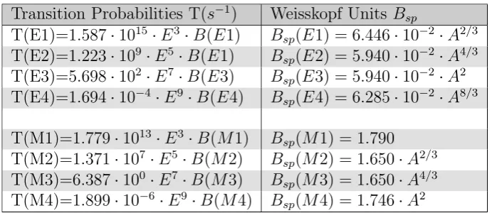
Table 2.1 shows expressions for the single-particle estimates for transition

(36)

Transition Probabilities T(s−1₎ _{Weisskopf Units} _B

sp

T(E1)=1.587·1015_·_E3_·_B₍_E₁₎ _B

sp(E1) = 6.446·10−2·A2/3

T(E2)=1.223·109_·_E5_·_B₍_E₁₎ _B

sp(E2) = 5.940·10−2·A4/3

T(E3)=5.698·102·E7_·_B₍_E₃₎ _B

sp(E3) = 5.940·10−2·A2

T(E4)=1.694·10−4·E9_·_B₍_E₄₎ _B

sp(E4) = 6.285·10−2·A8/3

T(M1)=1.779·1013_·_E3_·_B₍_M₁₎ _B

sp(M1) = 1.790

T(M2)=1.371·107 _·_E5_·_B₍_M₂₎ _B

sp(M2) = 1.650·A2/3

T(M3)=6.387·100 _·_E7_·_B₍_M₃₎ _B

sp(M3) = 1.650·A4/3

T(M4)=1.899·10−6·E9 _·_B₍_M₄₎ _B

[image:36.595.125.471.126.276.2]

sp(M4) = 1.746·A2

Table 2.1: Transition probabilities T (s−1_{) for Weisskopf single particle}

esti-mates expressed asB(EL) andB(ML). The energiesE are measured in MeV [Rin04]

2.7.2 Internal Conversion

An excited nucleus can decay to a lower energy state by the emission of a

γ ray. There are other processes that compete with γ-ray emission, one of

which is the emission of a conversion electron. Conversion-electron emission

is a process whereby the nucleus interacts with a bound atomic electron,

causing this electron to be ejected from the atom. This process is completely

separate from β decay, in which an electron is emitted from the nucleus

via the decay of a neutron into a proton, an electron, and an electron

anti-neutrino.

As this process is the result of a two-body interaction with a transition

between two well defined states, the energy imparted on the electron will be

well defined. This is not the case inβdecay, where the emitted electron has a

range of allowed energies owing to the three bodied nature of the interaction.

Atomic electrons are in bound states; the strength of this binding depends

(37)

[image:37.595.229.367.127.275.2]

Electron Shell B (keV) K 152.970 L1 30.038 L2 29.103 L3 22.359 M1 7.930 M2 7.474 M3 5.860 M4 5.176 M5 4.876

Table 2.2: Table of atomic electron binding energies for the innermost tran-sitions in lawrencium [Fir99]

of the electron will not be the same as the γ ray resulting from the same transition. The kinetic energy of the emitted electron, Te, can be described

by

Te = ∆E−B. (2.31)

The binding energy B, will depend on the shell from which the electron is ejected, i.e. the K, L, M, . . . shells. Table 2.2 shows the binding energies

for the innermost transitions in lawrencium. The difference in strength

be-tween the competing γ-ray emission and conversion-electron emission can

vary dramatically; one process may dominate or they can be much closer in strength. The probability of each decay mode occurring, for a given

transi-tion, is described by the internal conversion coefficient, α, which is defined as

the relative probabity of the decay occuring via conversion-electron emission

versus γ-ray emission.

α= Ne

Nγ

= λe

λγ

(38)

where λ denotes the decay probability of the respective decay mode. From,

this the total electromagnetic decay rate can be written as

λt =λγ(1 +α) =λγ(1 +αK+αL1+αL2+. . .). (2.33)

Internal conversion coefficients for a point nucleus can be defined as

α(EL)∼= Z

3

n3 L L+ 1

e

2

4π0hc¯

4 2mec 2

E

L+5/2

, (2.34)

for electric multipoles and

α(EL)∼= Z

3

n3 e2

4π0¯hc

4 2mec 2

E

L+3/2

, (2.35)

for magnetic multipoles [Kra87].

Some general trends of internal conversion coefficients can be drawn from

Equations 2.34 and 2.35.

• Internal conversion increases rapidly with nuclear charge (atomic num-ber Z).

• Internal conversion decreases with increasing transition energy (E).

• The probability for internal conversion increases for higher L transitions (L).

• The probability for internal conversion decreases for higher atomic shells (n).

(39)

[image:39.595.110.457.170.411.2]

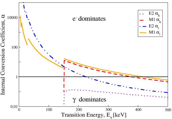
Figure 2.6: Internal conversion coefficientsαkandαtot, as a function of energy

for E2 and M1 transitions in lawrencium.

transitions could be completely unseen in γ-ray spectroscopy but strong in

electron spectroscopy.

Figure 2.6 details the conversion coefficients as a function of energy for

M1 and E2 transitions, for both K and total conversion. It is interesting to note that K conversion cannot occur below the K binding energy of the

given nucleus, in this case lawrencium. It is also clear how strongly low

(40)

Chapter 3 Experimental Methods

3.1 SAGE Spectrometer

The SAGE spectrometer [Pap10] consists of the JUROGAM II germanium detector array coupled to a solenoidal magnet which transports conversion

electrons to the SAGE silicon detector.

3.1.1 JUROGAM II array

The JUROGAM II array [Bea96] consists of 24 fourfold segmented Clover

dectors [She99], and 15 EUROGAM Phase I type Compton-suppressed

ger-manium detectors [Nol94, Bea92], though to accommodate the solenoidal

magnet of SAGE, 5 of these Phase I detectors need to be removed leaving 10

(41)

[image:41.595.195.413.398.621.2]

Figure 3.1: Schematic Diagram of the setup at Jyv¨askyl¨a, showing JU-ROGAM II and the SAGE silicon detector along with RITU and GREAT [Pap09].

(42)

[image:42.595.197.416.132.347.2]

Figure 3.3: Schematic drawing of the SAGE silicon detector showing the arrangement of the pixels.

3.1.2 SAGE silicon Detector

The SAGE silicon detector is a highly segmented detector made up of 90

pixels. The detector is 48 mm in diameter with a thickness of 1 mm. Fig-ure 3.3 shows the arrangement of the pixels along with dimensions and the

numbering scheme used.

3.1.3 SAGE Solenoidal Magnet and High Voltage

Bar-rier

The SAGE solenoidal magnet consists of three separate solenoids, two

up-stream of the target position and a third downup-stream. The upup-stream solenoids

(43)

Figure 3.4: Schematic of the RITU gas filled separator.

Doppler broadening of the electron peaks, along with reducing the amount of delta electrons incident of the detector, which are emitted with a heavy

forward focus. The solenoid magnets transport electrons from the target

po-sition to the detector, which is popo-sitioned upstream just off beam axis and at

a distance of ∼95 cm. Further to the solenoidal magnet, there is a high volt-age barrier in position between the target and the detector. When a negative

voltage is applied to this, it has the effect of suppressing the transmission of

low energy electrons, further reducing the background from delta electrons.

3.2 RITU Gas-filled Recoil Separator

RITU is a gas-filled recoil separator [Lei95], consisting of three quadrupole

(44)

ure 3.4 shows a schematic plan of the RITU gas filled separator, showing the

target chamber, the four magnets, and the GREAT focal plane array.

3.3 GREAT Focal Plane Array

The GREAT Focal Plane Array [Pag03], is a combination of silicon,

germa-nium, and gas detectors, for detecting the arrival and subsequent decay of

reaction products. It is sensitive to α particles, β particles, γ rays, X-rays,

as well as electrons from processes such as internal conversion and β

de-cay. GREAT consists of a number of separate detector systems that will be expanded upon in the following subsections. At the entrance to GREAT is

the multi-wire proportional counter (MWPC), next are the dual-sided silicon

strip detectors (DSSDs), 11.4 mm behind this is the planar detector. In a

box configuration around the DSSDs are the PIN diodes. Originally behind,

but now above this, is the GREAT Clover detector, further to this another

two fourfold segmented Clover detectors are placed either side. Figure 3.5

shows a schematic view of the GREAT focal plane spectrometer. Visible are the DSSD, PIN diodes, planar and the GREAT clover. Not shown are the

MWPC and the additional two Clover detectors.

3.3.1 Multi-wire proportional counter

The MWPC, is positioned at the entrance of GREAT. All products passing

through RITU to the focal plane, pass through it, allowing for identification

based on energy loss in the gas along with time of flight in conjunction with

(45)

Figure 3.5: Schematic of the GREAT Focal Plane Array [Pag03].

wide strut in the centre to support the thin mylar foils, used as the anode,

with the wires acting as the cathode. The MWPC is filled with isobutane

gas, this facilitates a small amount of energy loss by particles passing through

it. Particles can then be differentiated depending on their energy loss. This

ability to identify recoils passing through the MWPC allows for distinction between these and their subsequent radioactive decays.

3.3.2 Double-sided Silicon Strip detectors

The DSSDs, are the implantation detectors, each DSSD is 60 × 40 mm in size with a thickness of 300µm, with a strip width of 1 mm. Two of these

(46)

on one side and 40 horizontal strips on the other, giving a total of 4800 pixels.

The two DSSDs are mounted 4 mm apart on a hollow block through which

coolant is circulated, cooling the DSSDs to -20◦C. The detection efficiency for

recoils is∼85%. Further to detecting recoils with a high efficiency the DSSDs can detect α particles with an efficiency of ∼50% and conversion-electrons depending on the gain settings used.

3.3.3 Planar detector

The planar detector is a double-sided germanium strip detector, for measur-ing low energy γ-rays and X-rays. The detector has an active area of 120

× 60 mm and a thickness of 15 mm. The width of the strips on both sides is 5 mm. The efficiency of the Planar detector, along with the Clover

detec-tors is shown in Figure 3.6. These efficiencies are based on the GEANT4

simulation from Andreyev et al. [And04].

3.3.4 Silicon PIN photodiode detectors

An array of 28 silicon PIN photodiode detectors are mounted in a box

ar-rangement around the DSSDs, in the backwards direction relative to the

beam direction. Each of these PINs has an area of 28 ×28 mm and a thick-ness of 500µm. This arrangement has an efficiency of ∼20% [And04].

3.3.5 Clover detectors

(47)

[image:47.595.132.486.130.395.2]

Figure 3.6: Efficiency curve for various components in the GREAT focal plane array - obtained from [GJ08].

also tapered by an angle of 15◦ on the outside surface. Each crystal has

a further four fold segmentation. There is also a suppression shield of

bis-muth germanate crystals surrounding the detector to improve peak-to-total ratio. Further than the GREAT clover detector there are two more four fold

(48)

Chapter 4 Simulation of the SAGE

spectrometer in GEANT4

4.1 Justification of Simulation

As with any new detector setup, understanding its behaviour is a large part

in analysing any experiment performed with it. A comprehensive simulation not only allows better understanding of the performance of the setup, but can

be used as a tool to help in the tuning of such things as the electromagnetic

fields with the aim of increasing electron transmission efficiency.

During the design and construction phase of the SAGE spectrometer,

simulations were carried out using the SOLENOID code [But96]. These

simulations were limited to two dimensions with cylindrical symmetry and

focussed only on electron transport. The SOLENOID code did have the ability to specify an angle between the beam axis and the field axis, but not

(49)

symmetric field.

GEANT4 [Ago03] is a toolkit for the simulation of the passage of particles

through matter. It has a large range of functionality including reproduction

of complex geometry and materials alongside detailed physics models for

the interactions of particles with matter over a wide range of energies. The toolkit is implemented in the object-oriented programming language C++

and has been used in a wide range of applications in fields such as high energy

physics, nuclear physics, space engineering and medical physics.

A GEANT4 simulation overcomes the restrictions of the previous

simu-lation by being fully three dimensional and can also be expanded to include

the JUROGAM II array. This allows for a more realistic simulation and a

more detailed view of electron motion within SAGE and the volumes where

electrons are being lost [Pap12, Cox13].

4.2 Construction of the Geometry

The accuracy to which the geometry is reproduced is of great importance for the usefulness of the simulation. Figure 4.1 shows the simulated geometry.

The Phase I and Clover Ge detectors have been reproduced from design

specifications, including the bore hole, Li contacts, Ge crystals, BGO crystals,

Heavymet collimators, and supports. Figure 4.2 shows a cross section view

through two Clover and one Phase I Ge detectors.

Figure 4.3 shows the comparison between the simulated Si detector and

(50)

Figure 4.1: Complete Simulation of SAGE spectrometer, with the SAGE silicon detector to the left and JUROGAM II array to the right.

strips. This leads to a total inactive area of around 4%. For more in depth

discussion on the SAGE silicon detector see [Pap10].

Figure 4.4 shows a comparison between the simulated high voltage barrier

and the real one. The real high voltage barrier did not have the horseshoe connector, which is used to charge the high voltage barrier, fitted in this

(51)

Figure 4.2: Cross section view of two Clover(centre, right) and one Phase I (left) Ge detectors.

(52)

(53)

4.3 Analysis of Simulation Data

The ROOT data analysis framework [Bru97] has been used for the extraction

and analysis of data from the simulation. Within the simulation a ROOT tree

is built containing relevant details about each event. These details are mainly focussed on the values that are measurable in the real setup, namely the

energy deposition within detectors, but also include quantities that cannot

be measured such as,

• initial energies of particles

• initial momentum vector, for analysis of angular emission

• energy deposition in non-detector volumes, e.g. target wheel. This allows for in depth analysis of where efficiency losses occur, see section

4.5

• information of particles generation, i.e. primary particle, secondary particle generated from some physical process such as pair-production.

Once this ROOT tree has been generated all subsequent analysis can be

performed afterwards with the use of ROOT codes much faster than running the simulation. This is done as the tracking of several million electrons in

electromagnetic fields can take many hours, whereas generating a histogram

filled with the electrons detected in a certain volume, such as a single pixel

(54)

techniques such as Compton suppression and add-back can be implemented

also.

4.4 Tuning electromagnetic fields

GEANT4 has a number of models to describe charged-particle motion in an

electromagnetic field depending on the kind of motion, the accuracy of

sim-ulation needed and the type of field in question. Further to this there are a

number of parameters used to describe the required accuracy of the particle

motion in a given field. Here there is a trade-off between the accuracy of the simulation and the speed at which it can be performed. The initial

simu-lation and generation of the electromagnetic field map was performed using

the OPERA simulation package [Fie07]. This simulation was performed to

an accuracy of 1 cm in a 3D grid setup. The field map used covered an area

of 30 cm × 30 cm × 150 cm containing all volumes that electrons could be located within. More details on the field simulations can be found in [Pap10].

This meant that the field did not extend for the full simulation, rather only where the electrons of interest are likely to be affected by it. Further to

this, outside of the vacuum, where the Ge detectors are located, necessarily

had to be a low field region as the Ge detectors are highly sensitive to

elec-tromagnetic fields. To this end, a large number of shielding configurations

were tested, in simulations before construction, with the final setup, and

fi-nally in GEANT4. Figure 4.5 shows a schematic view of the final shielding

(55)

Shields

Solenoid axis

Beam axis

0 10cm

Figure 4.5: Schematic view of the magnetic coils and shielding within SAGE.

Figure 4.6: Comparison of electron distribution for original detector position (left) and detector moved by 10 mm towards the beam axis (right).

Initially the effect of the 3.2◦ angle between the upstream and downstream

coils, as can bee seen in Figure 4.5, was underestimated. This caused the

focus of the electrons to be off centre on the detector. This was reproduced

in GEANT4, as can be seen in Figure 4.6 where the initial distribution and

the final distribution of electrons can be seen.

(56)

intensity. To this end, the size and arrangement of the pixels within SAGE

was chosen with the aim of giving an even count-rate across the whole

detec-tor, with central, smaller pixels experiencing a higher intensity than outer,

larger pixels, which in turn detect more electrons due to their size.

The smallest aperture that electrons pass through in the SAGE spec-trometer is the carbon foil unit, which is necessary for separating the high

vacuum needed for operation of the high voltage barrier from the He gas

used in RITU, which has an inner diameter of 31 mm. The field map has

been interpolated from a 1 cm3 _{grid. From this scale it can be seen that}

us-ing greater than millimetre accuracy would not give a gain in accuracy and

would only increase the time taken for the simulation considerably.

In GEANT4 the motion of a charged particle in an electromagnetic field

is tracked by integration of it’s equation of motion. This is done using a Runge-Kutta method, there are other methods for specific types of fields

depending on their level of uniformity and whether they are wholly magnetic

in nature. The integration method is described by the stepper in GEANT4.

1

A number of parameters are used to describe how accurately the path of

a particle is tracked in GEANT4. A curved path of motion is broken down

into a series of linear chord segments, of length set by the user, that closely approximate the curved path. The distance of closest approach between a

volume boundary and a linear chord segment is known as the miss distance

or chord distance. If this chord distance is below a certain value, again set by

1_{The 4CashKarpRKF45 stepper was chosen for the best balance between reproduction}

(57)

the user, the path of motion will be recalculated with shorter steps, limited in

size by another parameter, to see if the particle will cross the boundary. At

which point if the particle is found to cross the boundary the interaction will

be calculated. These various parameters were all set to a value of 1 mm due to

the accuracy of geometry and field values, anything greater than this would increase significantly the computational time required without meaningful

change to accuracy.

4.5 Detection Efficiency

The most important aspect of the simulation is the accuracy with which

it reproduces the real experimental efficiency. For the real detector 133_Ba

and 209_{Bi are used for calibration as these give a spread of electron energies}

up to ∼1 MeV, see Section 5.1 for more on calibration of the SAGE silicon detector. With the simulation, it is a simple task to generate a given number

of electrons with a definite energy. For a detailed analysis of the detection

efficiency electrons are generated with energy divisions of 10 keV from 10 to 1000 keV. Through the use of ROOT, electrons with a given initial energy

can then be selected. As can be seen from Figure 4.7 electrons with initially

identical energies will lose varying amounts whilst being transported to the

detector. This can be caused by energy loss in the carbon foils for instance.

Figure 4.7 shows all electrons detected for an initial energy of 100 keV.

Of these a significant fraction have lost a large amount of their initial energy.

(58)

re-Figure 4.7: Simulated electrons in the SAGE silicon detector with an initial energy of 100 keV.

produced. This consists of a thin mylar window on the face pointing towards

the detector and a thicker acrylic backing pointing away. Electrons emitted

towards the detector lose a small amount of energy exiting the source and are

found in the main peak, electrons emitted at a backwards angle which are

reflected by the magnetic field lose a larger amount of energy and make up

the second lower energy peak. If only the number of electrons detected was taken as a measure of the efficiency, it would be a great overestimation, and

in a realistic case where there would be more than one energy peak and it

would not be possible. Ideally all the electrons in the peak would be counted

and those that would be considered background if it were real data would

be discounted. To achieve this a fitting algorithm was developed

combin-ing a Crystal Ball Function [Gai82] to fit the peak with a combination of a

quadratic and a step function to fit the background. It can be seen that the

(59)

line shows the combined step function and the quadratic. This is close to

what would be expected for fitting a real peak with this kind of background.

The need for this background subtraction diminishes as the energy of

the emitted electron increases, and is required even less for γ rays, but for

[image:59.595.148.437.282.489.2]

consistency purposes all fits are done using the same algorithm.

Figure 4.8: Simulated efficiency curve for the SAGE silicon detector com-pared to measured values for peaks in 133Ba and 207Bi.

Figure 4.8 shows a simulated efficiency curve for electrons of energies from

0 to 1000 keV. It can be seen that for energies below 200 keV this simulation

underestimates the electron efficiency, but for higher energies there is a good

agreement. The source of this discrepancy is not yet understood and it may

(60)

[image:60.595.151.437.163.370.2]

Figure 4.9: Simulated SAGE silicon detector efficiency as a function of high-voltage barrier setting.

ting. It can be seen that the efficiency below 200 keV is affected by the high-voltage barrier settings. The effect of the high-voltage barrier is

pre-dictable and proportionate to the barrier setting.

Figure 4.10 shows a comparison of simulated and measured efficiency for

a barrier setting of -30kV. Here it can be seen that there is a good

agree-ment with measured efficiency for energies above 200 keV, below this there is

still some difference between simulation and measured values, though from

50 keV downwards there is once again good agreement between simulation of measurement.

Alongside the detection efficiency of electrons with the SAGE silicon

(61)

[image:61.595.149.438.162.370.2]

Figure 4.10: Comparison of measured and simulated SAGE silicon detector efficiency for a high voltage barrier setting of -30kV.

important part of this simulation. Figure 4.11 shows a comparison of simu-lated and measured efficiency for the JUROGAM II array. It can be seen that

there is a very good agreement in shape between simulation and measured

efficiency, though in the simulation the efficiency is between 1-2 % higher at

all points. The reason for this is likely to do with a combination of

geom-etry not yet included in the simulation, namely the aluminium holder the

target wheel sits in, the motor used to rotate the wheel and tin and copper

absorber foils on the faces of the Phase I and Clover detectors, and inaccu-racies in crystal size and position. Though the effect seems too pronounced

(62)

fur-Figure 4.11: Simulated efficiency of the Jurogam II array also shown in blue is a calculated efficiency curve.

that has not been taken into account is the effect of low energy noise. For real detectors a threshold signal limit has to be set to stop excessively high

count rates. The effect this has on low energy efficiency could account for

the discrepancies seen here.

4.5.1 Efficiency Losses

The SAGE spectrometer has a number of apertures between the target

po-sition and the silicon detector, through which electrons must pass. This is

illustrated in Figure 4.12. Table 4.1 details the volumes that electrons deposit

energy in.

[image:62.595.148.437.163.370.2]

(63)

[image:63.595.150.458.144.363.2]

Figure 4.12: Simulation detailing the geometry near to the target position in SAGE, visible are the carbon foil unit, target wheel, target, and the detector chamber.

the target wheel, shown in Figure 4.12, that are the main volumes for

ab-sorbing electrons. The target also shows a very high number of interactions,

though it should be noted that these are generally of a very small energy and most electrons that interact here will go on to deposit most of their energy

in either the target wheel, carbon foil unit, or detector. Inversely, the target

chamber, detector chamber, and high-voltage barrier all account for a very

A GEANT4 simulation of the SAGE spectrometer and its first application to 255Lr