Analysis of bending wave transmission using beam tracing with advanced statistical energy analysis for periodic box-like structures affected by spatial filtering

Analysis of bending wave transmission using beam tracing

with advanced statistical energy analysis for periodic box-like

structures affected by spatial filtering

D. Wilson, C. Hopkins

n

Acoustics Research Unit, School of Architecture, University of Liverpool, Liverpool, United Kingdom

a r t i c l e i n f o

Article history: Received 12 April 2014 Received in revised form 3 November 2014 Accepted 20 December 2014 Handling Editor: D. Juve Available online 14 January 2015

a b s t r a c t

For bending wave transmission across periodic box-like arrangements of plates, the effects of spatial filtering can be significant and this needs to be considered in the choice of prediction model. This paper investigates the errors that can occur with Statistical Energy Analysis (SEA) and the potential of using Advanced SEA (ASEA) to improve predictions. The focus is on the low- and mid-frequency range where plates only support local modes with low mode counts and the in situ modal overlap is relatively high. To increase the computational efficiency when using ASEA on large systems, a beam tracing method is introduced which groups together all rays with the same heading into a single beam. Based on a diffuse field on the source plate, numerical experiments are used to determine the angular distribution of incident power on receiver plate edges on linear and cuboid box-like structures. These show that on receiver plates which do not share a boundary with the source plate, the angular distribution on the receiver plate boundaries differs significantly from a diffuse field. SEA and ASEA predictions are assessed through comparison with finite element models. With rain-on-the-roof excitation on the source plate, the results show that compared to SEA, ASEA provides significantly better estimates of the receiver plate energy, but only where there are at least one or two bending modes in each one-third octave band. Whilst ASEA provides better accuracy than SEA, dis-crepancies still exist which become more apparent when the direct propagation path crosses more than three nominally identical structural junctions.

&2014 Elsevier Ltd. Published by Elsevier Ltd. This is an open access article under the CC BY license (http://creativecommons.org/licenses/by/4.0/).

1. Introduction

Many engineering structures are regular in form, with repeating cellular units across which it is necessary to be able to predict bending wave transmission. For some periodic structures the bending wavelength of interest is much larger than the structural dimension between adjacent units. However, there is also a class of engineering problems where all the constituent structural elements that form the cellular unit, such as beams or plates, support local bending modes of vibration. In these situations it is usually assumed that the vibration field on the source subsystem approximates a diffuse field when the response to broadband excitation is multimodal in frequency bands. Under this assumption, Statistical Energy Analysis (SEA) is often used to predict structure-borne sound transmission[1]. However, even when there is an

Contents lists available atScienceDirect

journal homepage: www.elsevier.com/locate/jsvi

Journal of Sound and Vibration

http://dx.doi.org/10.1016/j.jsv.2014.12.029

0022-460X/&2014 Elsevier Ltd. Published by Elsevier Ltd. This is an open access article under the CC BY license (http://creativecommons.org/licenses/by/4.0/).

n_{Corresponding author. Tel.:þ44 1517944938.}

approximation to a diffuse field on the source subsystem, successive structural junctions between cellular units will filter the range of wave angles that are transmitted, leading to non-diffuse fields on the subsystems that form more distant cellular units.

To account for spatial filtering and the existence of non-diffuse vibration fields, Langley[2,3]proposed an alternative to SEA for the prediction of high-frequency vibration, Wave Intensity Analysis (WIA). A finite Fourier series was used to represent the directional dependency of the wave intensity. The application of power balance at the junction between plates leads to a set of simultaneous equations which can be solved to give the plate energy levels. Heron[4]proposed an alternative approach using ray tracing, which was referred to as Advanced Statistical Energy Analysis (ASEA). This was primarily developed to allow the inclusion of tunnelling mechanisms between indirectly-connected subsystems but as with WIA it also accounts for spatial filtering, non-diffuse vibration fields and propagation losses. Note that ASEA and WIA both converge on the same result. Heron noted that implementation of ASEA for coupled plates“could well turn out to be computationally expensive”compared with classical SEA (i.e. using wave theory to calculate the coupling loss factors) due to the ray tracing requirement. For this reason an alternative approach, referred to as‘beam tracing’is introduced in this paper to reduce computation times. The structures used for validation were a linear chain of rods with ASEA [4] and linear chains of plates with WIA [2,3]. These were essentially waveguides that were not representative of typical automotive, aeronautic, marine or building structures. Engineering constructions that are used for noise control tend to be formed from coupled plates where all or most plate edges are coupled to other plates to form open or closed box-like structures. Hence this paper focuses on systems consisting of a large number of plates in a box-like arrangement.

For coupled plate structures, Bercin[5]compared WIA and SEA against an exact approach based on dynamic stiffness to assess the importance of in-plane wave generation at junctions. It was noted that the structures were limited to those where two opposite plate edges were simply supported because of the requirements of the dynamic stiffness technique. However, the results confirmed that WIA gave better agreement with exact results from the dynamic stiffness technique than SEA, particularly with a linear chain of 15 coupled plates.

ASEA was used by Yin and Hopkins[6]to investigate tunnelling on an L-junction comprising a periodic ribbed plate with symmetric ribs and an isotropic homogeneous plate. Indirect coupling was significant at high frequencies where bays on the ribbed plate can be treated as individual subsystems. With excitation of the isotropic homogeneous plate, classical SEA gave significant underestimates in the energy of the bays due to the absence of tunnelling mechanisms. In contrast, ASEA gave close agreement with Finite Element Methods (FEM) and laboratory measurements. The errors incurred with SEA rapidly increased as the bays become more distant from the source subsystem. ASEA provided significantly more accurate predictions by accounting for the spatial filtering that led to non-diffuse vibration fields on more distant bays.

This paper investigates the effect of spatial filtering with periodic box-like structures formed from plates to demonstrate the errors that can occur when using SEA and assesses the potential of using ASEA to improve predictions. The focus is on the low- and mid-frequency range where (a) the plates support bending modes without any in-plane wave generation at the junctions, (b) low mode counts can cause problems with the application of SEA[7,8]and (c) the in situ modal overlap is relatively high due to the plates that form the boxes being coupled to several other plates. Previous comparisons of SEA with measurements on box-like structures have tended to show reasonable agreement[9,10]but conclusions cannot always be drawn due to the confounding effects of non-diffuse in-plane wave fields as well as unquantifiable variation in plate properties and junction properties[9], or relatively complex junctions with sufficient uncertainty in the damping that it was not possible to definitively validate the model [10]. To overcome this issue, this paper uses FEM models which have previously been validated against measurements on heavyweight walls and floors [11]. This avoids ambiguity about the internal damping and the coupling condition at the junction as these are prescribed in the FEM model.

2. Periodic box-like structures

2.1. Example structures for the FEM, SEA and ASEA models

Two periodic box-like structures are considered for the numerical experiments in linear and cuboid formats as shown in

Fig. 1. These structures represent buildings where the room volumes are 33.6 m3_{. To assess the implications of spatial}

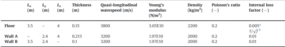
filtering for the modelling of sound transmission in buildings, all the plates that form these two structures represent heavyweight walls and floors. Similar types of repeating box-like structure has previously been used to assess aspects of structure-borne sound transmission in multi-occupancy types of residential accommodation[12,13]. Based on previous work [14], the absence of apertures (i.e. windows and doors) that would occur in a real building is assumed to make negligible difference for small apertures that are distant from the junction lines.Table 1contains the plate dimensions and the material properties for the masonry walls and concrete floors that were taken from previous measurements[15]. All analysis is carried out between 50 Hz and 1 kHz.

[image:3.544.62.488.65.556.2]

Fig. 1.(a) Linear box-like structure and (b) Cuboid box-like structure.

Table 1

Dimensions and material properties.

Lx (m)

Ly (m)

Lz (m)

Thickness (m)

Quasi-longitudinal wavespeed (m/s)

Young's modulus

(N/m2

)

Density

(kg/m3

)

Poisson's ratio

()

Internal loss

factor ()

Floor 3.5 – 4 0.15 3800 3.05E10 2200 0.2 0.005a

1/√fb

Wall A – 2.4 4 0.215 3200 1.97E10 2000 0.2 0.01

Wall B 3.5 2.4 – 0.1 3200 1.97E10 2000 0.2 0.01

a

For upper floors only.

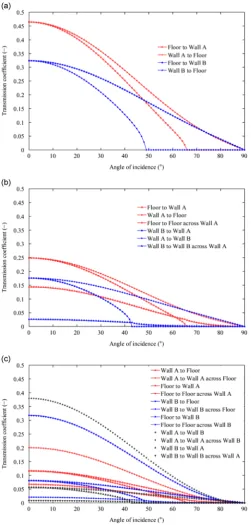
[image:3.544.41.508.608.685.2]

[image:4.544.149.401.153.680.2]

In this paper the models only allow bending wave transmission at the junctions. If in-plane wave generation was allowed it would be possible for in-plane modes to occur on each plate above the 500 Hz one-third octave band. However, previous work[16]on T-junctions of similar masonry walls indicates that in-plane wave generation only tends to make a significant difference to the out-of-plane response on the plates above 1 kHz. The bending wave transmission coefficients that are used for the SEA and ASEA models are determined from wave theory for semi-infinite plates[1,15]. Angular average transmission coefficients are used for the SEA models and angle-dependent values for the ASEA models. The angle-dependent values are shown inFig. 2indicating that the cut-off angles are between 431and 901.

2.2. Assessing the likely applicability of SEA

For the box-like structures described inSection 2.1, this section discusses parameters such as the mode count, modal overlap, attenuation within subsystems and weak coupling which are often used to make a preliminary assessment as to the applicability of SEA.

The fundamental bending modes for the floor (upper or ground), wall A and wall B occur at 37 Hz, 74 Hz and 37 Hz respectively, and the statistical mode counts for bending modes in one-third octave bands are shown inTable 2. From Fahy and Mohammed[7], SEA predictions for coupled plates using the wave approach tend to give reasonable estimates with low variance when the plates satisfy the empirical condition that in the frequency band of interest, the mode count is greater than or equal to five and the geometric mean of the modal overlap factors for the two plates is greater than or equal to unity. Over the frequency range between 50 Hz and 500 Hz, the mode counts are less than five for individual plates. However, by allowing for errors in an SEA prediction that are similar to those encountered from variation due to workmanship, Craik et al.[17]proposed more lenient conditions when using the wave approach (bending waves only) to calculate coupling loss factors in SEA. For a 3 dB error limit these conditions are for a modal overlap factor greater than 0.4 and mode counts greater than 0.5. At and above 100 Hz, these conditions are satisfied for the box-like structures considered in this paper.

In addition to mode counts it is clearly useful to try and quantify the modal overlap factor, but there are problems in that this requires knowledge of the total loss factor for the coupled plates. This has been estimated for the linear and cuboid structures by calculating the total loss factor as the sum of the internal loss factor and the coupling loss factors that are calculated using angular-average wave theory. These estimates are given inTable 3but should be considered as indicative of an upper limit. In fact, Mace and Rosenberg[18]have shown that modal overlap is not the most appropriate parameter to describe the effects of damping for rectangular plates. However, the modal overlap factor remains a practical and easily calculable parameter. For heavyweight building structures where each plate is coupled to several other plates, the more important issue concerning the variance of SEA estimates tends to be low mode counts rather than low modal overlap.

Although the primary interest in this paper concerns the effect of spatial filtering, the choice of a heavyweight building for the periodic box-like structures creates an opportunity to assess the ability of SEA and ASEA to predict the response of highly-damped subsystems in the form of concrete ground floors that are built on top of the soil[15]. From Lyon and DeJong

[1]the maximum dimension of a subsystem,Lmax, to prevent significant losses as waves propagate across the subsystem can

be determined according to

Lmaxo cg

ωη

(1)

wherecgis the group speed for bending waves and

ηj

is the internal loss factor. For the highly-damped ground floor, the actual plate dimensions are 3.5 m by 4 m andLmaxis 10.2 m; hence this inequality is satisfied for all the walls and floors.

[image:5.544.41.509.493.554.2]

For predictive SEA, there has been much debate about the need for (and the definition of) ‘weak’coupling between directly connected subsystems. A review of the SEA literature on weak coupling by James and Fahy[19]suggests that in seeking to define weak coupling there has been confusion between the validation of the fundamental SEA equations, the use of SEA with wave theory calculation of the coupling loss factor, and the requirements necessary to use experimental SEA. This has led to different definitions of weak coupling depending upon the model under consideration. The review concluded

Table 2

Statistical mode counts in one-third octave bands.

One-third octave band centre frequency (Hz)

50 63 80 100 125 160 200 250 315 400 500 630 800 1k

Floor 0.5 0.6 0.8 1.0 1.2 1.6 2.0 2.5 3.1 3.9 4.9 6.2 7.9 9.8

Wall A 0.3 0.4 0.4 0.6 0.7 0.9 1.1 1.4 1.8 2.2 2.8 3.5 4.5 5.6

Wall B 0.5 0.7 0.8 1.0 1.3 1.7 2.1 2.6 3.3 4.2 5.2 6.6 8.4 10.5

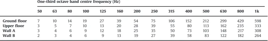
Table 3

Modal overlap factors in one-third octave bandsaverage value based on the total loss factor for the fully coupled plates calculated using angular-average wave theory.

One-third octave band centre frequency (Hz)

50 63 80 100 125 160 200 250 315 400 500 630 800 1k

Ground floor 7 10 14 19 27 39 54 75 106 152 212 299 429 598

Upper floor 3 5 7 10 13 20 28 39 55 80 113 162 235 333

Wall A 3 4 6 9 12 18 25 35 50 73 103 148 217 308

[image:5.544.46.512.618.690.2]

that weak coupling definitions that were created to assess the validity of the fundamental SEA equations are of little or no use. The approach proposed by Smith[20]defined weak coupling as occurring between two coupled subsystems when the internal loss factor is much larger than the coupling loss factor. Numerical analysis of two coupled plates by Le Bot and Cotoni[21]provides a useful reminder that the errors incurred when Smith's criterion for weak coupling is not satisfied, tend not to be as important as when subsystems have high damping, low modal overlap or low mode counts. An inherent problem with Smith's criterion is that it considers an SEA system comprising only two coupled subsystems. For the box-like structures that are considered in this paper, each plate subsystem is coupled to between four and ten other plate subsystems. Hence for the walls and the upper floor, the total loss factor is primarily determined by the sum of the coupling loss factors and is at least twice, and at most 29 times the value of the internal loss factor. Therefore Smith's criterion which considers the internal loss factor, rather than the total loss factor, is of little use in identifying issues with the validity of SEA due to a lack of weak coupling.

3. Advanced SEA

3.1. Theory

Advanced SEA was introduced by Heron[4]hence only the main aspects of the theory are introduced here. All the ASEA equations are developed in terms of modal energy,ej, for subsystemjas

ej¼Ej=nj (2)

whereEjis the subsystem energy andnjis the modal density in modes per rad/s.

The SEA power balance equations forNsubsystems can then be written in terms of modal energy as

M11 0 0 ⋯ 0

0 M22 0 ⋯ 0

0 0 M33 ⋯ 0

⋮ ⋮ ⋮ ⋱ ⋮

0 0 0 ⋯ MNN

2 6 6 6 6 6 6 4 3 7 7 7 7 7 7 5 e1 e2 e3 ⋮ eN 2 6 6 6 6 6 6 4 3 7 7 7 7 7 7 5 þ

A11 A12 A13 ⋯ A1N A21 A22 A23 ⋯ A2N A31 A32 A33 ⋯ A3N

⋮ ⋮ ⋮ ⋱ ⋮

AN1 AN2 AN3 ⋯ ANN 2 6 6 6 6 6 6 4 3 7 7 7 7 7 7 5 e1 e2 e3 ⋮ eN 2 6 6 6 6 6 6 4 3 7 7 7 7 7 7 5 ¼

Win;1 Win;2 Win;3 ⋮ Win;N 2 6 6 6 6 6 6 4 3 7 7 7 7 7 7 5 (3)

whereWin,jis the input power to subsystemj, andMis a diagonal matrix of modal overlap factors (defined using the

internal loss factor,

ηj

) as given by

M¼

ω

n1

η

1 0 0 ⋯ 0

0

ω

n2

η

2 0 ⋯ 0

0 0

ω

n3

η

3 ⋯ 0

⋮ ⋮ ⋮ ⋱ ⋮

0 0 0 ⋯

ω

nN

ηN

2 6 6 6 6 6 6 4 3 7 7 7 7 7 7 5 (4)

andAis a matrix of coupling loss factors,

ηij

, given by

A¼

XN

j¼2

ω

n1

η

1j

ω

n2

η

21

ω

n3

η

31 ⋯

ω

nN

ηN

1

ω

n1

η

12

XN

j¼1;a2

ω

n2

η

2j

ω

n3

η

32 ⋯

ω

nN

ηN

2

ω

n1

η

13

ω

n2

η

23

XN

j¼1;a3

ω

n3

η

3j ⋯

ω

nN

ηN

3

⋮ ⋮ ⋮ ⋱ ⋮

ω

n1

η

1N

ω

n2

η

2N

ω

n3

η

3N ⋯

XN

j¼1;aN

ω

nN

ηNj

2 6 6 6 6 6 6 6 6 6 6 6 6 6 6 6 6 6 6 6 4 3 7 7 7 7 7 7 7 7 7 7 7 7 7 7 7 7 7 7 7 5 (5)

are related to the input power through the equations

AeþMe¼P (6)

BeþMd¼Q (7)

where the elements ofAcontain the available power to available power transfers per unit modal energy and the elements of matrixBcontains the available power to unavailable power transfers per unit modal energy. In the absence of available to unavailable power transfers the ASEA equations are identical to classical SEA. The power balance is satisfied because each column ofAþBmust sum to zero.

Depending on the form of excitation, the input power in each subsystem is allocated as available and/or unavailable power per unit modal energy. For rain-on-the-roof excitation which is considered in this paper,Q¼0; hence combining Eqs.(6) and (7) gives

MþA

ð ÞðMBÞ1

M eð þdÞ ¼P (8)

This results in an SEA-like relationship between the total modal energy in each subsystem and the power input,

C eð þdÞ ¼P (9)

where the ASEA matrix,C, is defined as

C¼ðMþAÞðMBÞ1

M (10)

The elements ofA and Bare determined using an iterative ray tracing algorithm to calculate the power exchanges between subsystems. TheAandBmatrices are inserted into Eq.(9)to give the ASEA matrix which is then inverted to give the total modal energies of each subsystem in response to a prescribed power input vector, Pusing Eq.(9). The ASEA solution converges on a final value when all the most significant power exchanges between subsystems have been accounted for. This will occur at a finite iteration number which is here defined as ASEAN. All ASEA iterations between zero andNare labelled ASEA0 to ASEANto indicate the number of times power has been traced across the source subsystem. Note that ASEA0 is identical to the result from classical SEA.

3.2. Beam tracing

Previous work[6]using ASEA on two coupled plates tracked the power flow using a ray tracing procedure; these were rectangular plates for which each plate had only a single junction line and three perfectly reflecting boundaries. However, applying this form of ray tracing to a large number of coupled plates would result in excessive computation times. For example, even with just a few coupled plates, reflected and transmitted rays are generated each time an incident ray intersects the junction line. Hence the number of rays that needs to be tracked doubles at an L-junction (two plates), and trebles at a T-junction (three plates). To reduce the calculation time an alternative method is introduced here which will be referred to as‘beam tracing’. Rather than divide the perimeter into small segments of width, dL, and carry out numerical integration around the perimeter of the source plate, it is more efficient to divide the source plate into its constituent edges and use a beam tracing approach to determine the integrals. Hence the tracing of individual rays at each segment dLalong a single edge of the source plate is replaced by a pair of rays at each end of the edge which defines a‘beam’of rays. However there will still be an exponential growth in the number of beams with increasing ASEA iteration number. This occurs because transmitted and reflected beams are generated each time a beam‘illuminates’the junction line. The ASEA solution converges when the number of ASEA iterations approaches the total number of subsystems in the model[4,6], hence, for large numbers of coupled plates there is a need to reduce the growth in the number of beams with ASEA iteration number otherwise the total number of beams will rapidly become unmanageable. This is achieved by combining all the beams that are incident on a junction line within a small range of angles into a single beam.

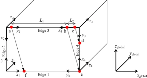
Local and global coordinate systems are needed to facilitate the tracing of the beams across the plates–see the example coordinate systems onFig. 3. Transformation matrices which describe rotations and translations between the global and local (i.e. subsystem) coordinates systems are used to track the beams as they are transmitted from one subsystem to another. This process is simplified by using a third set of edge coordinates for which thex-axis lies along the direction of the junction line. Transformation from the subsystem to the edge coordinates simplifies the application of Snell's law for the transmission of beams between plates. This is because thex-component of the transmitted beam can be set equal to thex -coordinate of the incident beam. The outward propagating component of the transmitted beam is always in the positive direction perpendicular to the junction line which can then be calculated using

ky¼ ffiffiffiffiffiffiffiffiffiffiffiffiffiffiffiffiffik2B k

2 x q

(11)

3.3. Calculation procedure

The built-up structure under analysis is sub-divided into plate subsystems that are characterised by their material and geometrical properties. The ASEA calculation involves five main steps in which the power flow is tracked around the structure and the available and unavailable powers are added to theAandBmatrices respectively. The ASEA calculation requires that these steps are repeated for every angle of incidence, on every section of the perimeter of every plate subsystem. These steps are described below and applied according to the flow chart inAppendix A.

Step1: Assuming a diffuse field on plate subsystemidue to the initial available power input, the power incident on a section of the plate perimeter,L, per unit modal energy,ei, within a narrow angular range d

θ

is given by

dWin;i ei ¼

kB;iL

4

π

2 cos

θ

d

θ

(12)

The initial free power input at an angle,

θ

, taken from the perpendicular to the section of the plate perimeter,L, is added to matrix element Aii. The transmitted and reflected power can then be calculated by multiplying Eq. (12)by the appropriate transmission or reflection coefficient. Note that ASEA0 (which is equivalent to SEA) only uses step 1 and does not use steps 25.

Step2: Generate a set of initial beams associated with each of the transmitted or reflected powers calculated in step 1 or from the previous ASEA iteration. The set of beams forms a two dimensional indexed array containing all information required to trace the beams.

Step3: This step involves tracing the beam across each subsystem. When a beam travels across a subsystem, different sections of the beam can‘illuminate’different edges and they will generally travel different distances before reaching the perimeter of the plate. As an example, consider the assembly of rectangular plates shown inFig. 3.

The two rays comprising the beam travel from points a and c of one edge, and intersect the perimeter again at points f and d respectively. The ray travelling from point a to point f intersects edge 1 and the ray travelling from point c to point d intersects edge 4. Point e is the intersection point between the lines representing edge 1 and edge 4. Point b is the intersection point between the line representing edge 3 and a line with the same slope as the ray that passes through the point e. When all points have been determined the beam is divided into two sections. The fraction of the initial power,

Wstart, entering each section is determined by the ratio,L1/(L1þL2). To describe the fraction of power lost in each section,

Heron [4] introduced an average damping factor, D, to account for different parts of the wave travelling different distances as it crosses the plate from one edge to another, given by

D¼_d 1

maxdmin

Z dmax

dmin

exp

ωη

_cx

g

dx¼exp ð

ωηi=

cg;iÞdmin

expð

ωηi=

cg;iÞdmax

ð

ωηi=

cg;iÞdmaxð

ωηi=

cg;iÞdmin

(13)

wheredminis the minimum distance anddmaxis the maximum distance between the initial edge and the intersected

edge in each section. The fraction of power lost in each section is added to matrix elementBji. The remaining power is available for further tracking.

Step4: This step concerns generation of transmitted and reflected beams along illuminated edges of subsystemj. The power incident on each of the plate edges is calculated and the transmitted and reflected powers can be found by applying the appropriate intensity transmission (or reflection) coefficient. The ASEA procedure returns to step 3 until all beams in the set have been traced.

Step 5: This step combines all Koutward going beams from step 4 that originate from the same edge of the same subsystems with the same heading into a single beam. The issue of an exponentially increasing number of rays is addressed by combining beams within the same subsystem that emanate from the same edge with the same heading

Edge 1 Edge 3

Edg

e 4

L1 L2

f

a b c

[image:8.544.149.390.57.185.2]

d xglobal yglobal zglobal x1 z1 y1 y2 z2 x2 y4 z4 x4 e Edg e 2 y3 x3 z3

into a single beam. Therefore the sum of all the power in a subsystem leaving a common boundary with the same heading is averaged into a single beam before returning to step 2 for the next ASEA iteration. When processing the final ASEA iteration the power of the outgoing rays in subsystemjthat is generated in step 4 is treated as‘residual power’and added to matrix elementAji. The initial coordinates of the resulting combined beam are an average value of the initial coordinates of each pair of rays that define the beams that are weighted by the initial power of the beam,Wstart,k. As an

example, consider the beam inFig. 3for which the initial coordinates of the two rays are [0,ak] and [0,ck]. This results in a set ofKbeams each emanating from the same edge as these rays with the same heading, the average coordinates of each ray, [0,a] and [0,c], in the beam are given by

0;a

½ ¼PK 1

k¼1Wstart;k

XK

k¼1

Wstart;k½0;ak (14)

0;c

½ ¼PK 1

k¼1Wstart;k

XN

k¼1

Wstart;k½0;ck (15)

When the subsystems represent rectangular plates this considerably reduces the total number of beams with high ASEA iteration numbers because it combines all the beams in each subsystem which repeat the same pattern of reflections into a single equivalent beam.

When the final ASEA iteration number has been completed, steps 15 are repeated for the next angle of incidence. Once all angles of incidence have been covered the process is repeated for all angles of incidence on the next edge of the subsystem perimeter. This process is repeated on the next subsystem for all angles of incidence, on all edges comprising the perimeter of the subsystem, until all subsystems in the model have been covered.

3.4. Convergence

ASEA calculations are carried out at one-third octave band centre frequencies with an angular resolution of 11. A convergence criterion is defined here as resulting in less than a 0.1 dB difference between ASEANand ASEAN–1 for the energy level difference from any combination of source and receiver subsystems. This means that if the rate of change of the energy level difference with ASEA iteration number remains constant then an additional ten iterations will only change the result by 1 dB. In fact the rate of change decreases with increasing ASEA iteration number so it will always be less than 1 dB. For the structures considered in this paper, this criterion results in an ASEA iteration number equal to the total number of subsystems plus four, which corresponds to ASEA30 and ASEA40 for the linear and cuboid box-like structures respectively. Based upon nominally the same criterion it is notable that for a linear chain of rods, Heron[4] proposed that the number of ASEA iterations should equal the number of subsystems minus two, and for a linear chain of plates, Yin and Hopkins[6]proposed it should equal the number of subsystems minus one. This indicates that convergence can occur more rapidly with linear chains of subsystems than with complex arrays of interconnected subsystems which are more typical of engineering structures.

4. Identification of spatialfiltering

To illustrate the effects of spatial filtering with the periodic box-like structures described inSection 2.1, it is instructive to assess the power incident on successive plate junctions when a diffuse field is applied to the source plate. The total incident power on a section of the junction line is obtained by projecting the intensity vector onto the junction line. The energy balance across the junction boundary ensures that the incident power equals the sum of the reflected and transmitted powers. Therefore conservation of power at each angle of incidence gives

Iinc;idLcos

θ

i¼Irefl;idLcos

θ

iþ

XJ

j¼2

Itran;jdLcos

θ

j (16)

where Jis the number of plates that form the junction (e.g. J¼2 for an L-junction, J¼3 for an T-junction,J¼4 for an X-junction).

For a diffuse field, the total power incident on the junction is given by the integral over all angles of incidence between

π

/2 and

π

/2, where

ItotaldL¼IincdL

Z π=2

π=2

[image:10.544.104.436.53.649.2]

and the power incident at a particular angle of incidence normalised to the total power incident on the junction is given by

IincdLcos

θ

i Itotal ¼

cos

θ

i

2 (18)

For ray tracing, a discretised form of Eq.(17)is used where the continuous range of angles is discretised into a set of angles,

θa

, each representing an angular band,

Δ

. The total power incident on the junction is

ItotaldL¼dL

XA

a¼1

Ibin;a

Δ

(19)

The incident power falling within a specified bin isIbin,a. In order to make a comparison with the diffuse field result in Eq.

(18), the power incident in a chosen band is normalised to the angular bin width and referenced to the total power incident on the junction as given by

Ibin;a

Δ

PA a¼1Ibin;a

(20)

For the two box-like structures, diffuse field excitation is applied to the upper floor of room 1 by allocating equal intensity in all directions such that the projection of the intensity onto the plate boundaries is related to the angle of incidence,

θ

, by cos

θ

. The beam tracing method is used to trace this initial power around the entire structure. The power incident on a particular plate edge within a range of angles corresponding to discrete bands of

Δ

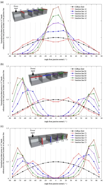
¼101is summed and divided by the total power incident at all angles. The number of beams incident on each edge is between 50,000 and 120,000. For the linear and cuboid box-like structures, the power ratios are shown in Figs. 4 and 5 respectively for comparison with an ideal diffuse field (Eq.(18)).

For junction lines on the excited plate the power ratio is approximately equal to that calculated for an ideal diffuse field. Compared to the ideal diffuse field the beam tracing results in slightly lower power ratios between 201and 201and slightly higher power ratios at angles greater than 20₁. This is caused by the rectangular shape of the source plate and the angular dependence of the reflection coefficients at the plate boundaries.

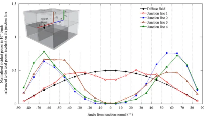
[image:11.544.114.442.474.660.2]

The extent of spatial filtering is clearly seen on the box-like structures. Referring back toFig. 2it is seen that the highest transmission coefficients occur at normal incidence and that many of them have cut-off angles between 431and 901such that there is no transmission at oblique angles close to grazing incidence. Across the upper floors of the linear structure, this results in the power ratio becoming progressively weighted towards normal incidence over successive junctions that are further away from the excited plate as shown inFig. 4(a). In contrast,Fig. 4(b) and (c) shows that for junctions with plates that are orientated perpendicular to the excited plate (i.e. the side walls), the power ratio rapidly decreases towards zero near normal incidence and increases to higher values than the ideal diffuse field at oblique angles. For the cuboid box-like structure, the same feature occurs with junctions on any non-excited plate as shown by the example inFig. 5.

Fig. 5.Cuboid box-like structure. Incident power per unit angle divided by the total incident power for different junction lines with 101resolution. Angles

5. Finite element methods

[image:12.544.58.481.171.668.2]

The finite element modelling is carried out using Abaqus software v6.10 on a high-performance computing cluster. The Abaqus direct method is used because the walls are made from different materials to the floors and the ground floors have a frequency-dependent internal loss factor. STRI3 elements are used which are three node triangular elements based on thin plate theory. The element size is assigned such that there are at least 10 nodes per free bending wavelength at the upper frequency of interest which corresponds to the upper frequency of the 1 kHz one-third octave band. The nodes along

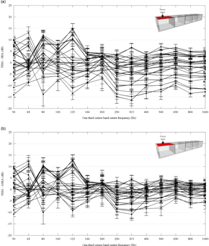
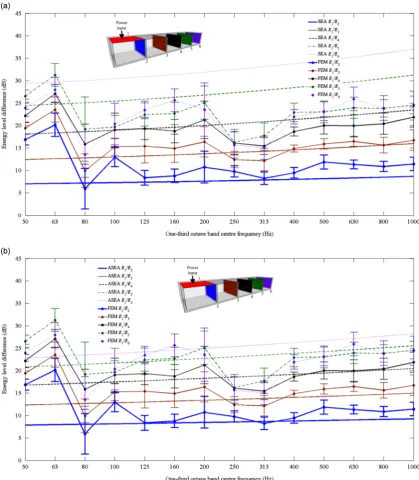
Fig. 6. Linear box-like structure. Difference between predicted energy level differences between the source plate and all receiver plates (a) FEM minus SEA

the plate junction line are constrained with all displacements set to zero such that there are only rotational degrees of freedom. This ensures only bending waves are generated at the plate junctions. Each plate has a prescribed internal loss factor which is related to a critical damping ratio and approximated by curve fitting the Rayleigh damping curve to the critical damping ratio in each one-third octave band. In terms of the Rayleigh coefficients

αR

and

βR

the critical damping ratio is

γ

¼

α

R

2

ω

þ

βRω

2 (21)

[image:13.544.60.485.183.670.2]

Rain-on-the-roof (ROTR) excitation is applied to the surface of the source plate using point forces with unity magnitude and random phase that are applied in a direction normal to the surface to the unconstrained nodes of the source plate.

Fig. 7. Cuboid box-like structure. Difference between predicted energy level differences between the source plate and all receiver plates (a) FEM minus SEA

[image:14.544.58.482.197.675.2]

The total power input and energy of each plate subsystem is calculated according to[15]. As the aim is to compare FEM with SEA and ASEA, a Monte-Carlo approach is used to generate an ensemble of FEM models where the subsystems have similar properties. This allows calculation of a mean response with a calculated standard deviation[15]. To introduce uncertainty into the ensemble, the quasi-longitudinal phase speed of the plates in the structure is randomly selected from a Normal distribution and different sets of ROTR excitation are used for each ensemble member. Fifteen ensemble members were generated using this procedure. Previous work[22]measured the quasi-longitudinal phase speed of a number of nominally identical masonry walls similar to Walls A and B. Based on these measurements, a standard deviation of 200 m/s is assumed for Walls A and B, and in the absence of data for concrete floors, the same is assumed for the floors. Any value lying more than three standard deviations from the mean was discarded. The quasi-longitudinal wavespeeds were then converted to a Young's modulus for the plates.

[image:15.544.63.483.186.667.2]

Solving for each member of the ensemble with a particular set of ROTR excitation applied to a particular plate in the structure gives a set of subsystem energies and input powers. Repeating the process a number of times using a different set of Young's modulus and ROTR forces generates an ensemble of subsystem energies. The subsystem energies and input powers are averaged between the upper and lower limits of one-third octave bands. Energy level differences in decibels are calculated between source and receiver subsystems for each ensemble member, and the ensemble-average energy level difference is given by the arithmetic average of these values.

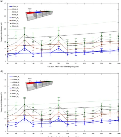
Fig. 9.Linear box-like structure. Energy level differences between the upper floor (source) and Wall A (receivers)comparison of FEM with (a) SEA and

6. Comparison of SEA, ASEA and FEM

FEM data are now used as a benchmark against which to compare SEA and ASEA models. FEM, SEA and ASEA are each used to predict the energy level difference between the source and receiver plates in terms of 10 log10(Esource/Ereceiver).

[image:16.544.59.482.193.667.2]

Although each structure has a large number of subsystems, the general trends can be assessed usingFigs. 6and7for the linear and cuboid structures respectively. For a chosen source plate and all possible receiver plates these graphs show the difference between the energy level difference predicted using FEM and the energy level difference predicted using SEA or ASEA. The results show that in comparison to SEA, ASEA provides significantly better estimates of the FEM prediction at frequencies at and above 200 Hz. For the linear box-like structure, the difference between the energy level differences in

Fig. 10.Linear box-like structure. Energy level differences between the upper floor (source) and Wall B (receivers)comparison of FEM with (a) SEA and

decibels for FEM minus ASEA tends to be in the range 75 dB (although there are individual values up to 11 dB) at and above 200 Hz. For the cuboid box-like structure, FEM minus ASEA results are between 5 dB and þ7 dB at and above 200 Hz, and73 dB in the 800 Hz and 1 kHz bands. Below 200 Hz the mode count in each one-third octave band tends to be less than two (seeTable 2) and in this region, ASEA gives no improvement over SEA.

6.1. Linear box-like structure

[image:17.544.62.486.193.664.2]

For the linear box-like structure,Figs. 8–11show the energy level difference between the source plate and successive receiver plates of the same type (i.e. upper floor, Wall A, Wall B, ground floor). The general trend is that ASEA predicts

Fig. 11.Linear box-like structure. Energy level differences between the upper floor (source) and the ground floors (receivers)comparison of FEM with

increasingly lower energy level differences than SEA as the receiver subsystem becomes increasingly distant from the source subsystem (i.e. with an increasing number of junctions between the source and receiver subsystems). As shown inSection 4, spatial filtering of the vibration field by successive junctions weights the transmitted power towards normal incidence. Therefore transmission across each junction becomes significantly larger than predicted by angular-average wave theory used in SEA. This results in ASEA showing closer agreement with FEM than SEA due to the fact that ASEA accounts for spatial filtering. For this structure, ASEA predicts energies for the furthest receiver plate that are up to 11 dB higher than those predicted by SEA.

[image:18.544.61.482.193.668.2]

The energy level differences from the upper floor (source) at one end of the structure to the other upper floors are shown inFig. 8. For the adjacent upper floor, SEA and ASEA predictions ofE1/E2fall within the 95% confidence intervals of the FEM

Fig. 12.Cuboid box-like structure. Energy level differences between a mid-floor and adjacent walls and floors comparison of FEM with (a) SEA and

ensemble for ten out of the fourteen one-third octave bands. This indicates that SEA can be valid for adjacent plates when there are low mode counts due to (a) the variation that exists for an ensemble of similar constructions, (b) the fact that wall A tends to provide a significant impedance mismatch between adjacent upper floors and (c) the modal overlap factors are significantly greater than unity. For upper floor 3, SEA and ASEA predictions ofE1/E3only fall within the 95% confidence

[image:19.544.61.486.192.668.2]

intervals of the FEM ensemble for six out of the fourteen bands. For upper floors 3, 4 and 5, the 95% confidence intervals of the FEM ensemble cluster together near the 125 Hz band and between the 250 Hz and 500 Hz bands. This clustering is not predicted by SEA or ASEA. Referring back toFig. 4(a) it is seen that the incident power ratio is predicted to be significantly weighted towards normal incidence on junction lines between upper floors 3 and 4, and upper floors 4 and 5. For upper floors 4 and 5 this results in ASEA giving lower energy level differences than SEA, but only four to six out of the fourteen

Fig. 13. Cuboid box-like structure. Energy level differences between a mid-floor and non-adjacent side walls (wall B)comparison of FEM with (a) SEA

bands fall within the 95% confidence intervals of the FEM ensemble. Whilst this might be expected below 200 Hz where the mode counts in each one-third octave band tend to be less than two, the discrepancy above 200 Hz between ASEA and FEM suggests that the cause could be due to neglecting phase effects with ASEA.

The energy level differences from the upper floor (source) to the walls that separate the rooms (wall A) are shown in

[image:20.544.59.481.193.665.2]

Fig. 9. For walls 2 and 3, SEA and ASEA predictions fall within the 95% confidence intervals of the FEM ensemble for five to eleven of the fourteen bands. However in the 250 Hz and 315 Hz bands there is strong coupling which is unaccounted for by ASEA; this leads to an overestimate of the energy level difference byE10 dB for walls 5 and 6 although a reason for this strong coupling has not been identified. For walls 4, 5 and 6, ASEA shows significantly closer agreement with FEM than SEA above 315 Hz. The improvement with ASEA is clearest for the furthest wall (wall 6) where SEA differs from FEM byE12 dB whereas ASEA only differs byE3 dB.

Fig. 14. Cuboid box-like structure. Energy level differences between a mid-floor and non-adjacent side walls (wall A)comparison of FEM with (a) SEA

The energy level differences from the upper floor (source) to the side walls (wall B) are shown inFig. 10. Above 200 Hz, both SEA and ASEA overestimate transmission from the upper floor (source) to the adjacent side wall (wall 2) by approximately 2.5 dB. Hence whilst ASEA gives closer agreement with FEM than SEA for walls 3, 4, 5 and 6, there is the possibility that this could be partly due to ASEA overestimating the energy in wall 2.

[image:21.544.62.485.198.676.2]

The energy level differences from the upper floor (source) to the ground floors are shown inFig. 11. For ground floor 2, ASEA provides a clear improvement over SEA between 125 Hz and 1 kHz. For ground floors 2, 3, 4 and 5, ASEA predictions fall within the 95% confidence intervals of the FEM ensemble for six to twelve of the fourteen bands. SEA significantly overestimates the energy level difference for the two furthest floors due to their high damping; SEA overestimates the energy level difference for the furthest floor byE14 dB whereas ASEA overestimates byE6 dB. Highly damped subsystems such as these ground floors tend to be considered problematic for inclusion in SEA, but ASEA is able to account for energy losses as waves propagate across them, as well as the effects of spatial filtering.

6.2. Cuboid box-like structure

For the cuboid box-like structure,Figs. 12–15show the energy level difference between the source plate and successive receiver plates of the same type. The energy level differences from a mid-floor (source) to some of the adjacent walls and floors are shown inFig. 12. For floors 5 and 6, both SEA and ASEA predictions fall within the 95% confidence intervals of the FEM ensemble for seven to eleven of the fourteen bands. In contrast, for walls 2, 3 and 4 this only occurs for two to seven of the fourteen bands. The energy level differences from a mid-floor (source) to some non-adjacent side walls (wall B) are shown inFig. 13and other non-adjacent side walls (wall A) inFig. 14. Above 200 Hz, ASEA gives improved agreement with FEM compared to SEA. The energy level differences from a mid-floor (source) to non-adjacent floors are shown inFig. 15. The results for upper floors 3 and 4 are similar whereas the energy of ground floor 2 is significantly lower due to its higher damping. For ground floor 2, both SEA and ASEA predictions fall within the 95% confidence intervals of the FEM ensemble for six to seven of the fourteen bands. The finding for floors 3 and 4 differ; compared to SEA, ASEA significantly improves the agreement with FEM for floor 4 but reduces the agreement with floor 3.

6.3. Linear and cuboid box-like structures

For both structures where the plate mode counts in each band were at least two, the energy level differences predicted using ASEA is typically within 3 dB of FEM for the plates that form the same room as the source plate or in the adjoining room whereas the error is typically 6 dB for SEA. However, for receiver plates that are directly coupled to the source plate, SEA is similar to ASEA with both approaches tending to underestimate the energy level difference by up to 3 dB.

For a diffuse vibration field, the transmitted power is weighted towards waves arriving at normal incidence on the junction. However for both SEA and ASEA the source plates under investigation have low mode counts. Based on the principle of wave-mode duality, waves will only be incident on the plate boundaries at the equivalent angles of the modes that are excited in each one-third octave band. For this reason, both ASEA and SEA tend to overestimate the energy for receiver plates that are directly connected to the source plate. Wester and Mace[23]have shown that use of angular-average wave theory overestimates the coupling between two finite rectangular plates.

7. Conclusions

ASEA has been used to investigate the role of spatial filtering on systems consisting of box-like arrangements of plates arranged in a repeating pattern. To increase the computational efficiency when using ASEA on large systems, a beam tracing method has been introduced which groups together all rays with the same heading into a single beam. This approach was used to determine the angular distribution of power that is incident on the plate edges on linear and cuboid box-like structures. On the source plate, the power incident on the plate boundaries was similar to a diffuse field. However, for receiver plates which do not share a boundary with the source plate, the angular distribution of power incident on the receiver plate boundaries differs significantly from the diffuse field prediction. The incident power becomes progressively weighted towards normal incidence for transmission over successive junctions arranged in a linear sequence. However, for successive receiver plates which are orientated perpendicular to the excited plate, the power ratio rapidly decreases towards zero near normal incidence and increases to higher values than the ideal diffuse field at oblique angles.

The numerical examples focussed on the low- and mid-frequency range where low mode counts can cause lower accuracy with SEA predictions that use wave theory to determine the coupling loss factors. Finite element methods were used to model the linear and cuboid box-like structures to provide a basis upon which to assess the efficacy of the SEA and ASEA predictions. With rain-on-the-roof excitation on the source plate, the results show that compared to SEA, ASEA provides significantly better estimates of the receiver plate energy, but only where there are at least one or two bending modes in each one-third octave band. At lower frequencies where there are lower mode counts, ASEA gives no improvement over SEA. There are also indications that for highly-damped plate subsystems such as the ground floors, ASEA provides closer agreement with FEM than SEA because ASEA is able to account for propagation losses.

The main implication for the prediction of structure-borne sound transmission over large distances in repeating box-like structures formed from plates (such as buildings) is that the effects of spatial filtering rapidly become apparent after only a few structural junctions. This results in vibration fields that can no longer be considered as diffuse. Whilst ASEA provides better accuracy than SEA, discrepancies still exist which become more apparent when the direct propagation path crosses more than three nominally identical structural junctions.

Acknowledgement

Appendix A

[image:23.544.173.384.98.678.2]

ASEA is implemented using the procedure outlined schematically inFig. A1.

References

[1]R.H. Lyon, R.G. DeJong,Theory and Application of Statistical Energy Analysis, Butterworth-Heinemann, MA, USA, 1995.

[2]R.S. Langley., A wave intensity technique for the analysis of high-frequency vibrations,Journal of Sound and Vibration159 (3) (1992) 483–502. [3]R.S. Langley, A.N. Bercin., Wave intensity analysis of high frequency vibrations,Philosophical Transactions of the Royal Society of London A346 (1994)

489–499.

[4]K.H. Heron, Advanced statistical energy analysis,Philosophical Transactions of the Royal Society of London A346 (1994) 501–510.

[5]A.N. Bercin., An assessment of the effects of in-plane vibrations on the energy flow between coupled plates,Journal of Sound and Vibration191 (5) (1996) 661–680.

[6]J. Yin, C. Hopkins, Prediction of high-frequency vibration transmission across coupled, periodic ribbed plates by incorporating tunnelling mechanisms,

Journal of the Acoustical Society of America133 (4) (2013) 2069–2081.

[7]F.J. Fahy, A.D. Mohammed, A study of uncertainty in applications of SEA to coupled beam and plate systems, Part 1: computational experiments,

Journal of Sound and Vibration158 (1) (1992) 45–67.

[8]C. Hopkins, Statistical energy analysis of coupled plate systems with low modal density and low modal overlap,Journal of Sound and Vibration251 (2) (2002) 193–214.

[9]R.J.M. Craik, A. Thancanamootoo, The importance of in-plane waves in sound transmission through buildings,Applied Acoustics37 (1992) 85–109. [10]T.J. Monger, K.H. Heron, A.P. Payne, J.M. David, L. Guillaumie, M. Menelle, A. Morvan, C. Soize, Statistical energy analysis predictions of the DOVAC box

experimental results,Proceedings of Euronoise98 (1998) 195–200.

[11] C. Hopkins, Vibration transmission between coupled plates using finite element methods and statistical energy analysis. Part 1: comparison of measured and predicted data for masonry walls with and without apertures,Applied Acoustics64 (2003) 955–973.

[12]C. Hopkins, M. Robinson, On the evaluation of decay curves to determine structural reverberation times for building elements,Acta Acustica United with Acustica99 (2013) 226–244.

[13]C. Hopkins, M. Robinson, Using transient and steady-state SEA to assess potential errors in the measurement of structure-borne sound power input from machinery on coupled reception plates,Applied Acoustics79 (2014) 35–41.

[14]C. Hopkins, Vibration transmission between coupled plates using finite element methods and statistical energy analysis. Part 2: the effect of window apertures in masonry flanking walls,Applied Acoustics64 (2003) 975–997.

[15]C. Hopkins.,Sound Insulation, Butterworth-Heinemann, Oxford, 2007.

[16]C. Hopkins, Experimental statistical energy analysis of coupled plates with wave conversion at the junction,Journal of Sound and Vibration322 (2009) 155–166.

[17] R.J.M. Craik, J.A. Steel, D.I. Evans, Statistical energy analysis of structure-borne sound transmission at low frequencies,Journal of Sound and Vibration

144 (1) (1991) 95–107.

[18]B.R. Mace, J. Rosenberg., The SEA of two coupled plates: an investigation into the effects of subsystem irregularity,Journal of Sound and Vibration212 (3) (1998) 395–415.

[19] P. James, F.J. Fahy, Weak coupling in statistical energy analysis, ISVR Technical Report No. 228, Institute of Sound and Vibration (ISVR), UK. February 1994.

[20] P.W. Smith, Statistical models of coupled dynamical systems and the transition from weak to strong coupling,Journal of the Acoustical Society of America65 (3) (1979) 695–698.

[21]A. Le Bot, V. Cotoni, Validity diagrams of statistical energy analysis,Journal of Sound and Vibration329 (2010) 221–235.

[22] C. Hopkins, Measurement of the vibration reduction index,Kijon free standing masonry wall constructions,Building Acoustics6 (1999) 235–257. [23] E.C.N. Wester, B.R. Mace, Statistical energy analysis of two edge-coupled rectangular plates: ensemble averages,Journal of Sound and Vibration193 (4)