common-envelope binary SDSS J1021+1744
.
White Rose Research Online URL for this paper:
http://eprints.whiterose.ac.uk/108489/
Version: Accepted Version
Article:
Irawati, P., Richichi, A., Bours, M.C.P. et al. (8 more authors) (2016) A large, long-lived
structure near the trojan L5 point in the post common-envelope binary SDSS J1021+1744.
Monthly Notices of the Royal Astronomical Society, 456 (3). pp. 2446-2456. ISSN
0035-8711
https://doi.org/10.1093/mnras/stv2810
[email protected]
https://eprints.whiterose.ac.uk/
Reuse
Unless indicated otherwise, fulltext items are protected by copyright with all rights reserved. The copyright
exception in section 29 of the Copyright, Designs and Patents Act 1988 allows the making of a single copy
solely for the purpose of non-commercial research or private study within the limits of fair dealing. The
publisher or other rights-holder may allow further reproduction and re-use of this version - refer to the White
Rose Research Online record for this item. Where records identify the publisher as the copyright holder,
users can verify any specific terms of use on the publisher’s website.
Takedown
If you consider content in White Rose Research Online to be in breach of UK law, please notify us by
arXiv:1511.09205v1 [astro-ph.SR] 30 Nov 2015
A large, long-lived structure near the trojan L5 point in
the post common-envelope binary SDSS J1021+1744
P. Irawati
1
,
⋆
A. Richichi
1
, M. C. P. Bours
2
, T. R. Marsh
3
, N. Sanguansak
4
,
K. Chanthorn
4
, J. J. Hermes
2
, L. K. Hardy
5
, S. G. Parsons
2
, V. S. Dhillon
5
,
6
,
S. P. Littlefair
5
1National Astronomical Research Institute of Thailand, 191 Siriphanich Bldg., Huay Kaew Road, Chiang Mai 50200, Thailand 2Departamento de F´ısica y Astronom´ıa, Universidad de Valpara´ıso, Avenida Gran Breta˜na 1111, Valpara´ıso, Chile
3Department of Physics, University of Warwick, Gibbet Hill Road, Coventry CV4 7AL, UK
4School of Physics, Suranaree University of Technology, 111 University Avenue, Muang, Nakhon Ratchasima 30000, Thailand 5Department of Physics and Astronomy, University of Sheffield, Sheffield S3 7RH, UK
6Instituto de Astrof´ısica de Canarias, 38205 La Laguna, Santa Cruz de Tenerife, Spain
Accepted 2015 November 27. Received 2015 November 27; in original form 2015 September 18
ABSTRACT
SDSS J1021+1744 is a detached, eclipsing white dwarf / M dwarf binary discovered in the Sloan Digital Sky Survey. Outside the primary eclipse, the light curves of such systems are usually smooth and characterised by low-level variations caused by tidal distortion and heating of the M star component. Early data on SDSS J1021+1744 obtained in June 2012 was unusual in showing a dip in flux of uncertain origin shortly after the white dwarf’s eclipse. Here we present high-time resolution, multi-wavelength observations of 35 more eclipses over 1.3 years, showing that the dip has a lifetime extending over many orbits. Moreover the “dip” is in fact a series of dips that vary in depth, number and position, although they are always placed in the phase interval 1.06 to 1.26 after the white dwarf’s eclipse, near the L5 point in this system. Since SDSS J1021+1744 is a detached binary, it follows that the dips are caused by the transit of the white dwarf by material around the Lagrangian L5 point. A possible interpretation is that they are the signatures of prominences, a phenomenon already
known from H
α
observations of rapidly rotating single stars as well as binaries. Whatmakes SDSS J1021+1744 peculiar is that the material is dense enough to block con-tinuum light. The dips appear to have finally faded out around 2015 May after the
first detection by Parsons et al.in 2012, suggesting a lifetime of years.
Key words: binaries: close – binaries: eclipsing – stars: white dwarfs – stars: indi-vidual: SDSS J102102.25+174439.9
1 INTRODUCTION
In recent years, primarily as the result of the Sloan Digital
Sky Survey (SDSS,York et al. 2000;Abazajian et al. 2009),
large numbers of white dwarf / main-sequence (WDMS)
bi-naries have been discovered (Rebassa-Mansergas et al. 2007,
2012,2013). A significant number of these have periods so
short that they must have emerged from a phase in which both stars orbited within the envelope of the white dwarf’s progenitor. During such “common envelope” phases, binary
orbital energy is lost to the envelope (Webbink 1984),
result-⋆ E-mail: [email protected]
ing in the observed short-periods (or often complete
merg-ing of the stars, Briggs et al. 2015). White dwarf /
main-sequence post common-envelope binaries (PCEBs) form a large, easily observed population for testing the outcome of the common-envelope phase, which is significant in the for-mation of many classes of close binary.
As the number of known PCEBs has increased, so too has the number of eclipsing systems. Thus, while in 2000 we
knew of just 5 eclipsing PCEBs (Marsh 2000, including the
a WDMS binary from the SDSS Data Release 7 and the stel-lar parameters of this binary were published as part of the online SDSS WDMS binary catalogue
(http://www.sdss-wdms.org,Rebassa-Mansergas et al. 2012). This binary was
also suspected as strong candidate PCEB from its radial velocity variability. The catalogue published an M4 type for the red dwarf star and a white dwarf with mass of
1.06±0.087M⊙. The effective temperature of the white
dwarf in J1021+1744 was given as ‘hot’ and ‘cold’ solution from the Balmer line profile fits. The white dwarf
tempera-tures are32595±928 K and17505±820K for the hot and
cold case, respectively.
The eclipsing nature of J1021+1744 was discovered by Parsons et al.(2013, P13 hereafter) from a search for pho-tometric variability of WDMS systems in Catalina Sky
Sur-vey (CSS, Drake et al. 2009, 2014) data. The eclipses are
of the white dwarf by its M dwarf companion and recur
with an orbital period of 0.14 days. Using the robotic
Liv-erpool Telescope (LT) in 2012 June, P13 found a drop in the brightness shortly after eclipse, about half as deep as the eclipse itself. This is highly unusual: outside eclipse, the vast majority of these systems show only slow varia-tions due to irradiation and tidal distortion. P13 showed a possible flare taking place before the white dwarf was fully out of the eclipse, leading them to suggest that the dip in flux might be caused by material ejected from the flare. They gave new constraints for the white dwarf mass us-ing their new ephemeris data, the measured radial velocity, and the mass function equation, lowering the estimated mass to 0.50±0.05M⊙. Rebassa-Mansergas et al. (2012)’s white dwarf mass was based upon model atmosphere fitting, made difficult because of the contamination of the white dwarf’s spectrum by its companion.
In this paper we present photometric observations of J1021+1744 taken mainly with the 2.4 m telescope at the Thai National Observatory, covering more than 30 eclipses from 2014 January to 2015 May in a variety of filters and with sub-minute time resolution. Our observations reveal that the dip observed by P13 is long-lived, with a lifetime of at least a few years. We also show that the dip is resolved into multiple components that vary both with time and wave-length. We suggest here that the dips originate from obscu-ration of the white dwarf showing that this detached binary is able to support dense clouds of material around the L5 trojan point.
2 OBSERVATIONS AND DATA REDUCTION
The bulk of our photometric data of J1021+1744 were taken using the 2.4 m Thai National Telescope (TNT) on Doi Inthanon, equipped with the ULTRASPEC camera. This facility is ideal for such studies, thanks to the combina-tion of high time resolucombina-tion, sensitivity and flexibility in time allocation. We supplemented this with a single eclipse observed with the high-speed triple-beam camera ULTRA-CAM mounted on the 4.2m William Herschel Telescope (WHT) on 2015 January 17. ULTRASPEC is based on a
low-noise 1k × 1k EMCCD frame-transfer detector, and is
described in detail byDhillon et al.(2014). During the first
observing cycle of TNT (2013 November – 2014 April), we monitored this star for 17 nights from 2014 January to April,
covering more than 20 eclipses in different filters. In the fol-lowing cycle (2014 November – 2015 May), we obtained 13 more eclipses from 9 nights of observations. The log of our
observations is presented in Table1.
Each observation consists of several hundreds to sev-eral thousands of frames, with the sampling times listed in
Table1. The detector integration times are 14.9 ms shorter
than the sampling times (see section 3.4 of Dhillon et al.
2014). The frame size is usually equal to the full
detec-tor window, although in some cases smaller windows are
adopted (e.g. 400×800 pixels). Each frame is accurately
time-stamped at mid-exposure thanks to a dedicated GPS system. The data are then processed using the ULTRACAM
pipeline (Dhillon et al. 2007). After bias subtraction and flat
fielding, the data are corrected to take into account the po-sition of the Solar System Barycenter. One or more refer-ence stars are recorded simultaneously with J1021+1744, allowing us to obtain accurate relative photometry. We note that the ULTRACAM pipeline includes adaptive estimates of seeing and star positions, and is thus very robust against changes in photometric quality, airmass, and tracking errors. For our observations we used several ULTRASPEC fil-ters which are similar to the passbands of the SDSS
pho-tometric system, namely g′,r′,i′,z′. Additionally, we used
the KG5 filter which is effectively equivalent to SDSS
u′+g′+r′(as described inDhillon et al. 2014), and the
self-explanatoryi′+z′filter. Finally, we also obtained data with
a clear filter (white light).
During the data processing we noticed several incon-sistencies in the depth of the primary eclipses. Eclipses in white dwarf binaries are wavelength dependent, and we real-ized that some of our light curves supposedly taken with the same filter appear to have different eclipse depths. Further investigations indicated that there were problems with the filter wheel rotation on some of our nights. In other words, the wheel did not move to the intended filter, without any alerts at the software level. We recovered from the problem as follows.
For each of the data sets with an ambiguous filters, we stacked all frames to create one deep image and examined all non-variable stars in the field. We then compared the fluxes against various sky surveys. Using this method we could identify the correct filter for all of our affected data. We also verified the eclipse depths by filter, as discussed in
Section3. The changes from nominal to adopted filters are
marked in Table1. The problem was fixed at the hardware
level in the summer of 2014 and is not present in later data.
In Table 1 we list the signal-to-noise ratio (SNR) as
computed over 10 minutes in the pre-eclipse part of the light curve, centered around phase 0.93. The numbers in the see-ing column are approximate values measured from the stellar profiles.
3 PHOTOMETRIC ANALYSIS
3.1 Light curve fitting
We implemented a light curve fitting method
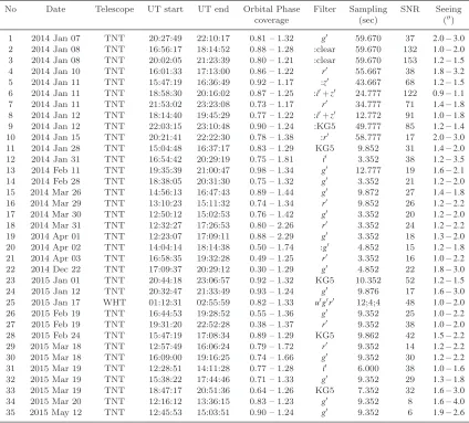
Table 1.Observation log of J1021+1744 obtained from TNT using ULTRASPEC and WHT with ULTRACAM. Each row represents one dataset where the start and the end of the exposure are given in columns 4 and 5, together with the corresponding orbital phase in column 6. The filters are listed in column 7. The presence of a colon before the filter denotes that the nominal filter name has been changed to an adopted filter, as explained in the text. Column 8 gives the exposure time of a single frame, where there is a dead time of 14.9 ms between exposures. In Column 9 and 10 we list SNR (measured in the pre-eclipse part; see text) and approximate seeing values for each run.
No Date Telescope UT start UT end Orbital Phase Filter Sampling SNR Seeing
coverage (sec) (′′)
1 2014 Jan 07 TNT 20:27:49 22:10:17 0.81 – 1.32 g′ 59.670 37 2.0−3.0
2 2014 Jan 08 TNT 16:56:17 18:14:52 0.88 – 1.28 :clear 59.670 132 1.0−2.0
3 2014 Jan 08 TNT 20:02:05 21:23:39 0.80 – 1.21 :clear 59.670 153 1.2−1.5
4 2014 Jan 10 TNT 16:01:33 17:13:00 0.86 – 1.22 r′
55.667 38 1.8−3.2
5 2014 Jan 11 TNT 15:47:19 16:36:49 0.92 – 1.17 :z′
43.667 68 1.2−1.5
6 2014 Jan 11 TNT 18:58:30 20:16:02 0.87 – 1.25 :i′+z′ 24.777 122 0.9−1.1
7 2014 Jan 11 TNT 21:53:02 23:23:08 0.73 – 1.17 r′ 34.777 71 1.4−1.8
8 2014 Jan 12 TNT 18:14:40 19:45:29 0.77 – 1.22 :i′+z′ 12.772 91 1.0−1.8
9 2014 Jan 12 TNT 22:03:15 23:10:48 0.90 – 1.24 :KG5 49.777 85 1.2−1.4
10 2014 Jan 15 TNT 20:21:41 22:22:30 0.78 – 1.38 :r′ 58.777 17 2.0−3.0
11 2014 Jan 28 TNT 15:04:48 16:37:17 0.83 – 1.29 KG5 9.852 31 1.4−2.0
12 2014 Jan 31 TNT 16:54:42 20:29:19 0.75 – 1.81 i′ 3.352 38 1.2−3.5
13 2014 Feb 11 TNT 19:35:39 21:00:47 0.98 – 1.34 g′ 12.777 19 1.6−2.1
14 2014 Feb 28 TNT 18:38:05 20:31:30 0.75 – 1.32 g′ 3.352 21 1.2−2.0
15 2014 Mar 26 TNT 14:56:13 16:47:43 0.89 – 1.44 g′ 9.872 27 1.4−1.8
16 2014 Mar 29 TNT 13:10:23 15:11:32 0.74 – 1.34 r′ 9.852 26 1.2−2.2
17 2014 Mar 30 TNT 12:50:12 15:02:53 0.76 – 1.42 g′ 3.352 20 1.2−2.0
18 2014 Mar 31 TNT 12:32:27 17:26:53 0.80 – 2.26 r′ 3.352 24 1.2−2.2
19 2014 Apr 01 TNT 12:23:07 17:09:11 0.88 – 2.29 g′
3.352 18 1.3−2.0
20 2014 Apr 02 TNT 14:04:14 18:14:38 0.50 – 1.74 :g′
4.852 15 1.2−1.8
21 2014 Apr 03 TNT 16:58:35 19:32:28 0.49 – 1.25 r′
3.352 16 1.0−2.2
22 2014 Dec 22 TNT 17:09:37 20:29:12 0.30 – 1.29 g′ 4.852 22 1.8−3.0
23 2015 Jan 01 TNT 20:44:18 23:06:57 0.92 – 1.32 KG5 10.352 52 1.2−1.5
24 2015 Jan 12 TNT 20:32:47 21:33:49 0.93 – 1.24 g′ 9.876 17 1.6−3.0
25 2015 Jan 17 WHT 01:12:31 02:55:59 0.82 – 1.33 u′g′r′ 12;4;4 48 1.0−2.0
26 2015 Feb 19 TNT 16:44:53 19:28:52 0.55 – 1.36 g′ 9.352 25 1.0−2.2
27 2015 Feb 19 TNT 19:31:20 22:52:28 0.38 – 1.37 r′ 9.352 38 1.0−2.0
28 2015 Feb 24 TNT 15:47:19 17:08:34 0.89 – 1.29 KG5 9.862 42 1.5−2.2
29 2015 Mar 18 TNT 12:57:49 16:06:24 0.79 – 1.72 r′ 9.352 14 1.2−2.2
30 2015 Mar 18 TNT 16:09:00 19:16:25 0.74 – 1.66 g′ 9.352 30 1.2−2.2
31 2015 Mar 19 TNT 12:28:51 14:11:28 0.77 – 1.28 i′ 6.000 38 1.0−1.6
32 2015 Mar 19 TNT 15:38:22 17:44:46 0.71 – 1.33 g′ 9.352 29 1.3−1.8
33 2015 Mar 19 TNT 18:47:17 20:51:36 0.64 – 1.26 KG5 7.352 32 1.6−3.0
34 2015 Mar 20 TNT 12:16:12 13:36:15 0.83 – 1.23 g′ 9.352 8 1.6−4.0
35 2015 May 12 TNT 12:45:53 15:03:51 0.90 – 1.24 g′ 9.352 6 1.9−2.6
an initial model. In this model, we allowed the inclination angle, the white dwarf and red dwarf radii, and the red dwarf temperature to vary, while the mass ratio and the white dwarf temperature are fixed. We have excluded those parts of light curves with dips and other variations during
the fitting process. The ‘hot’ solution with 32595 K for
the temperature of the white dwarf gives too strong a reflection effect in our model. On the other hand, the lower
temperature of 17505 K from the SDSS WDMS binary
catalogue is probably also not reliable (it has a very high
gravity of log(g) =9.5 and it is found at the edge of the
model grid), but must be closer to the correct value. Hence,
we chose the value of 17505 K for our model. The strong
contamination by the red dwarf and the faintness of the system are possibly the cause of the uncertainty in the temperature determination.
We also applied a Markov Chain Monte Carlo (MCMC) algorithm to confirm the result of the light curve fit. Using a
fixed mass ratio ofq=0.5with white dwarf temperature of
TWD=17505K, our best fit model gives an inclination angle
ofi=85◦. The radii of the two stars (scaled by the binary
separation) are RWD/a=0.0116 and Rsec/a=0.3572, with
the red dwarf companion almost filling its Roche Lobe. The temperatures of the red dwarf star derived from our model
isTsec=3160K. We then fitted each individual light curve
using the binary parameters given above, allowing only the orbital period and the time of mid-eclipse as free parameters.
3.2 Mid-eclipse times and new ephemeris
We first adopted the ephemeris from P13 to compute the
or-bital phase, where the oror-bital period isPorb=0.140359073(1)
days. The adopted ephemeris shows that the mid-eclipse is
offset earlier by∼3 min from the expected time. The derived
O−C values from ULTRASPEC data taken in late 2014 and
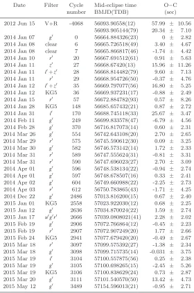
Table 2. The eclipse times for J1021+1744. For each date, we listed the filter names, cycle number, mid-eclipses, the O−C and the uncertainties in our O−C calculation in seconds. The eclipse times of the original and the new LT data are given in the first and second rows. For ULTRACAM data (2015 Jan 17), we list the weighted average of the mid-eclipse times from each filter.
Date Filter Cycle Mid-eclipse time O−C number BMJD(TDB) (sec) 2012 Jun 15 V+R -4068 56093.90558(12) 57.99 ± 10.56
56093.905144(79) 20.34 ± 7.10 2014 Jan 07 g′ 0 56664.884326(23) 0 ± 2.82 2014 Jan 08 clear 6 56665.726518(49) 3.40 ± 4.67 2014 Jan 08 clear 7 56665.866817(46) -1.74 ± 4.42 2014 Jan 10 r′
20 56667.691512(61) 0.91 ± 5.63 2014 Jan 11 z′
27 56668.67420(13) 15.96 ± 11.26 2014 Jan 11 i′
+z′
28 56668.814482(79) 9.60 ± 7.13 2014 Jan 11 r′
29 56668.954726(50) -0.37 ± 4.76 2014 Jan 12 i′+z′ 35 56669.797077(56) 16.80 ± 5.25
2014 Jan 12 KG5 36 56669.937231(17) -0.88 ± 2.49 2014 Jan 15 r′ 57 56672.884782(93) 0.57 ± 8.26
2014 Jan 28 KG5 148 56685.657432(21) 0.87 ± 2.72 2014 Jan 31 i′ 170 56688.745118(33) 25.67 ± 3.47
2014 Feb 11 g′ 249 56699.833578(47) -6.79 ± 4.56
2014 Feb 28 g′ 370 56716.817073(14) 0.60 ± 2.31
2014 Mar 26 g′ 554 56742.643108(20) 2.70 ± 2.65
2014 Mar 29 r′ 575 56745.590612(30) 0.09 ± 3.25
2014 Mar 30 g′ 582 56746.573142(14) 1.72 ± 2.33
2014 Mar 31 r′ 589 56747.555624(31) -0.81 ± 3.31
2014 Mar 31 r′ 590 56747.696023(27) 2.70 ± 3.09 2014 Apr 01 g′ 596 56748.538134(22) -0.94 ± 2.74 2014 Apr 01 g′
597 56748.678507(16) 0.33 ± 2.41 2014 Apr 02 g′
604 56749.660988(22) -2.25 ± 2.73 2014 Apr 03 r′
612 56750.783865(43) -1.71 ± 4.25 2014 Dec 22 g′ 2486 57013.816200(15) 0.67 ± 2.40
2015 Jan 01 KG5 2558 57023.922030(12) 0.68 ± 2.25 2015 Jan 12 g′ 2636 57034.870024(22) 1.59 ± 2.74
2015 Jan 17 u′g′r′ 2666 57039.0808021(41) 2.28 ± 2.02
2015 Feb 19 g′ 2906 57072.766864(12) -0.45 ± 2.23
2015 Feb 19 r′ 2907 57072.907249(20) 1.77 ± 2.66
2015 Feb 24 KG5 2941 57077.679420(20) -0.49 ± 2.67 2015 Mar 18 r′ 3097 57099.575392(27) -1.38 ± 2.34
2015 Mar 18 g′ 3098 57099.715735(14) -0.031 ± 3.75
2015 Mar 19 i′ 3104 57100.557875(56) 0.25 ± 2.38
2015 Mar 19 g′ 3105 57100.698265(15) -2.45 ± 5.26
2015 Mar 19 KG5 3106 57100.838629(24) 0.73 ± 2.87 2015 Mar 20 g′ 3111 57101.540570(50) 13.42 ± 4.73 2015 May 12 g′ 3489 57154.596013(21) -0.95 ± 2.71
used a light curve fitting method (as described above) to find the mid-eclipse timings for every light curve. The new orbital period resulting from our fitting process is shorter by almost 0.03 s and the new ephemeris derived from our data is
BMJD(TDB) =56664.8843262(231) +0.140358755(1)E
We list the mid-eclipse times in Table 2, including the
mid-eclipse of the LT light curve of P13. We have applied a barycentric correction to all of our times following a method
developed by Eastman et al. (2010), and we present these
numbers in BMJD(TDB). The O−C are derived with
re-spect to the T0 on 2014 January 7 (the date of the first
ULTRASPEC data obtained at TNT). In Figure1we
com-pare the O−C values calculated using P13’s orbital period
(left panel) with the values from our newly derived orbital period (right panel). P13’s LT data point is plotted as a filled square. Additionally, we fitted the LT light curve
us-ing our binary model and recalculated the O−C using our
ephemeris (presented as filled triangle). There is a 38 seconds difference between the original and the new LT mideclipse times. In their paper, P13 mentioned a flare which occured during the egress of the white dwarf (see Figure 5 of P13). This flare could have affected the fitting of the eclipse in P13. Since we know the width of the eclipse from our UL-TRASPEC data, we can exclude the flare in P13 data for our light curve fitting.
3.3 Dips in J1021+1744
We have detected for the first time clear evidence of multiple dips after the main eclipse in the light curve of J1021+1744,
as shown in Figure2. The light curves presented in the
fig-ure are theg′ filter data of our target and the comparison
Porb= 0.140359073d Porb= 0.1403587555d
−5000 −2500 0 2500 5000
Cycles
2013 2014 2015
−100 0 100
O-C
(seconds)
−5000 −2500 0 2500 5000
Cycles
2013 2014 2015
−20 0 20 40 60
O-C
[image:6.595.47.543.86.277.2](seconds)
Figure 1.O−C diagrams for J1021+1744 calculated using the old ephemeris of P13 (left) and our new ephemeris from ULTRASPEC data (right). The LT data from P13 is marked with a filled square. Our re-fitting result to the LT data using the ephemeris from ULTRASPEC data is marked with a filled triangle (see section3.2).
Ref J1021
0.8 0.9 1 1.1 1.2 1.3
Orbital phase
0 20 40 60 80 100
Time after start (min)
0 0.5 1
Normalised
flux
Figure 2.g′filter light curve of J1021+1744 from 2014 January
7, displaying the white dwarf eclipse and double dip from orbital phase 1.1 to 1.2. Each data point represents a single frame with exposure time 59 sec. The small gap around phase 0.89 is due to the rotation of the instrument during the exposure.
7. In this work, we present the light curves in terms of or-bital phase, using the ephemeris derived from ULTRASPEC
data. For reference, a 0.1 phase interval corresponds to∼20
minutes.
The flux scale is normalised and then rescaled to 1 out-side the eclipse and to 0 during the eclipse. We computed
the average values between the orbital phase0.9−0.95 and
0.97−1.03, and used the first phase range for our light curve
normalisation. The rescaling factor is the difference between the two average values. We chose to rescale our light curves to minimise the effect of the filters over our analysis of the dips (see below).
We used a similar approach for the light curve of the
comparison star shown in Figure2. We normalised the flux of
the comparison star to 1 using the average value in the same phase range mentioned above. The normalized comparison star’s flux is then offset to -0.3 for clarity.
The light curve of J1021+1744 clearly shows variations
after the white dwarf eclipse, around phase 1.1−1.2. The
drop in our light curve has two connected dips with different
depth. The system dims by∼50% during the first dip, and
becomes even fainter through the second dip, with more than 80% of the light of the white dwarf blocked. The star then slowly returns to its out-of-eclipse brightness around phase 1.2. The first dip seems to be consistent in phase and in am-plitude with that reported by P13. The second dip however was not present at all in the LT light curve. It should have been clearly evident as it is wider and deeper in our data than the first dip. We suspect that the second dip developed after the P13 observation in 2012 June. We will show later that these dips are evolving in shape and amplitude.
After the initial work to identify the correct fil-ter, the wavelength-dependence of the primary eclipses of J1021+1744 follow our expectations for this type of bina-ries. The eclipses are dominant in the blue and decrease in depth towards the red part of the spectrum. The trend in wavelength for the dip features is the same as in the main eclipse, and possibly even more pronounced. The dips are obscuration of the white dwarf, hence the similarity in the wavelength dependency between the eclipses and the dips. Later data taken (simultaneously) using ULTRACAM show
that the dips are deepest in the u′ band, as illustrated in
Figure3. The ULTRACAMu′band data were taken with a
longer exposure time compared to theg′ orr′ filters,
there-fore we have smaller number of datapoints in theu′ band
light curve. For these data, the sampling in theu′ filter is
three times slower than in the other filters. We normalised the flux scale to the average value of the pre-eclipse section
only (phase0.90−0.95) to show the relative shape and the
depth of the white dwarf eclipses. We would like to note that the ULTRACAM data definitely confirms the dip depths as a function of wavelength, as the ULTRASPEC data were taken in different orbits for different filters.
The dips are clearly seen in the g′ filter, though they
appear to be less prominent at this wavelength. They are
shallower inr′ and KG5 filters, and barely visible in thei′
andi′+z′filters. This may suggest that the material causing
[image:6.595.43.281.338.489.2]u′
g′
r′
0.9 1 1.1 1.2 1.3
Orbital phase 0
0.5 1 0 0.5 1
Normalised
flux
[image:7.595.42.281.73.282.2]0 0.5 1
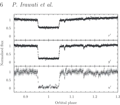
Figure 3.Light curve of J1021+1744 taken on 2015 January 17 from the WHT telescope with ULTRACAM. From top to bottom the filters arer′,g′, andu′. The data inu′has fewer points due to longer exposure time. The light curves are normalised to the aver-age flux between phase 0.9−0.95. The white dwarf eclipses follow the expected pattern where they are deeper at bluer wavelengths. The dip features seem to follow a similar trend.
Our next task was to examine the dips profile. Since the mid-eclipse times are known, the location of the dips can be determined accurately. In our 2014 data, the dips were prominent and were always located between phase 1.10 and 1.25. Multiple number of dips are recorded in every light curve, often with complex shapes. We present the light
curves obtained between 2014 January−April in Figure 4,
focusing on the section where the dips are visible. The light curves are ordered in time from top to bottom. We exclude
the data in thei′,z′,i′+z′filters because the dips are faint in
these wavelengths, as well as the data taken in the night of
2014 April 3. Our target was setting with airmass>2during
our observation on 2014 April 3, and the part of light curve
with dips is heavily affected by noise. Figure4shows 18 light
curves and the flux of each light curve has been rescaled to
0 and 1, as in Figure2. For the nights where we used a short
exposure time (<5s), the data points are binned to show
more clearly the profile of the dips.
The analysis of the dips in J1021+1744 is quite challeng-ing, due to the fact that they were evolving rapidly in time
(as seen in Figure4) and in shape, from one simple structure
into a complex one or vice versa. We decided to mark the well-visible dips, but only those which can be seen in almost every light curve. We used a numbering system from 1 to 5 based on their position in orbital phase. The number can be followed by letters a, b, and c for a dip which is split into a few smaller dips (in the case of dip 1).
Dips 1 and 3 are always present in our 2014 data. We
marked dip 1 as ‘1b’ for the first seven light curves, and
then assign the letters ‘a’ and ‘b’ after it split into two nar-row dips. Dip 2 was marked for the first time on 2014 Jan 15, although, it is possible that this dip was already present in the light curves prior to this date. However, the long ex-posure used for the first few light curves does not allow us to resolve this dip. Dips 4 and 5 were not present at all at the beginning of our observations. They first emerged on 2014
January 28 and then disappear and reappear throughout 2014. There were two occasions where another dip appeared between dips 1 and 2, which was on March 30 and April 1.
This dip is marked as ‘1c’. Dip1c is a fine example to show
the swift evolution of the dips. On the night of 2014 April 1, we observed J1021+1744 uninterruptedly for 5 hours, fol-lowing two eclipses in orbital cycle 596 and 597. During this observation, we witnessed the appearance of dip 1c in cycle 597, blocking half of the total light from the binary for more than two minutes. Such a dip was not recorded in the light curve of cycle 596.
We followed the same procedure to mark the dips in our
2015 data (Figure5). It is obvious that the dips which were
present in our 2015 light curves are different from those that appeared in our 2014 data. We obtained our first data of the second observing season on the night of 2014 December 22. The dip was absent from this light curve. A small dip seems to be visible at phase 1.07 on 2015 January 1 and January 12. However, we are not certain of this because it lies far (in phase) from the previous known dips in this system. It is also only marginally significant given the errors and the fluctuations in the light curves. Our WHT+ULTRACAM data, which was taken four nights later, confirmed the pres-ence of this small dip. This light curve also revealed a second
shallow dip at phase∼1.15 and possibly even a third dip at
phase∼1.22. Our further TNT observations show that only
dip 2 which remains present in our subsequent 2015 data.
4 DISCUSSION
Our data set is sufficiently extended, and the number and positions of the dips sufficiently complex, that it is difficult to provide a detailed discussion of each feature. However, we can discuss in broad terms at least the time scale of the phenomenon and the time evolution of the dips, in order to infer some conclusions.
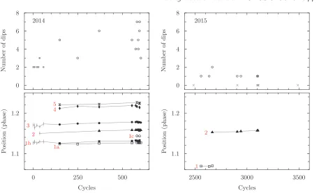
We counted the total number of dips in each light curve
based on the markings given in Figure4and5, where each
mark represent one dip. In some light curves we assigned
‘a1b’ and this mark is counted as two dips. The result is
shown in Figure6(top panels). In 2014, we found that there
are dips in every light curve, starting with two and increas-ing to about five or more by 2014 April. The actual num-ber varies from day to day, even from one cycle to another.
The light curves with the highest number of dips are theg′
. Apr 2 -g′
. Apr 1 -g′
. Apr 1 -g′
. Mar 31 -r′
. Mar 31 -r′
. Mar 30 -g′
. Mar 29 -r′
. Mar 26 -g′
. Feb 28 -g′
. Feb 11 -g′
. Jan 28 - KG5
. Jan 15 -r′
. Jan 12 - KG5
. Jan 11 -r′
. Jan 10 -r′
. Jan 8 - clear . Jan 8 - clear
. Jan 7 -g′
2014 1a
a1b a1b a1b a1b a1b a1b a1b a1b
1a a1b
1b
1b
1b
1b
1b
1b
1b
3 3
3 3 3 3 3 3 3 3 3 3 3 3 3 3 3
2 2 2 2 2 2 2 2 2 2
4 4 4
4 4 4
4 4
5 5 5 5 5
1c
1c
1.05 1.1 1.15 1.2 1.25
Orbital phase 0
1 2 3 4 5 6 7 8 9 10 11 12 13 14 15 16 17 18 19
Normalised
[image:8.595.110.481.99.707.2]flux
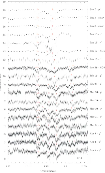
Figure 4.A close up look of the light curves of J1021+1744 (2014 data) between phases1.05−1.26. The light curves are arranged from the oldest at the top to the newest at the bottom. Some data with short exposure times are binned for clarity. The dips in our 2014 light curves clearly evolves in shape, width, and depth. We mark the position of each dip with numbers from 1 to 5. In some light curves where dip 1 is split into three smaller dips, we annotated them with1a,1band1c. Each mark represents one dip, except fora1bwhere
. May 12 -g′ . Mar 19 - KG5
. Mar 19 -g′
. Mar 18 -g′
. Mar 18 -r′
. Feb 24 - KG5
. Feb 19 -r′
. Feb 19 -g′
. Jan 17 -g′
. Jan 12 -g′
. Jan 1 - KG5
. Dec 22 -g′
2015 1
1
1 2
2
2
2
2
1.05 1.1 1.15 1.2 1.25
Orbital phase 0
1 2 3 4 5 6 7 8 9 10 11 12 13
Normalised
[image:9.595.90.496.94.451.2]flux
Figure 5.Similar to Figure 4, but for the data obtained in 2015 observing season. The first data were taken on 2014 December 22. Only one or two small dips are seen in some light curves. The light curves with the highest time-resolution have been binned for clarity.
April and December, then their minimum lifetime would be at least 1.5 years. A connection with the first detected dip by P13, implying a lifetime of several years, seems more difficult
to defend. We recall the case of QS Vir (O’Donoghue et al.
2003), in which two deep dips were detected before the
pri-mary eclipse. However, further observations did not detect the dips again, pointing to a short-lived phenomenon.
In Figure6we also plot the position of the dips in the
2014 and 2015 data (bottom panels). To measure the posi-tions, we visually inspected each dip and tried to determine the minimum of each feature, unless they had an asymmetric shape. In this case we used the position of the data points with the lowest flux. Our analysis shows that all dips were shifting towards later orbital phase, although, small varia-tions exist in the early 2014 data. From this plot we can infer that the dips are not stationary with respect to the orbital phase of the binary. It might also imply that the ma-terial is slowly drifting away from the binary. We measure a shift of 0.01 in orbital phase for dip 3, or almost 2 minutes in time. Despite having different characteristics (in depth, width, and numbers), the dips from our 2015 datasets also show similar behaviour. The fact that the dips are multiple and are shifting in phase leads to the conclusion that the material is in the form of several blobs, which are orbiting the red dwarf but at the same time subject to varying
gravi-tational forces which change their relative position from the star and among themselves.
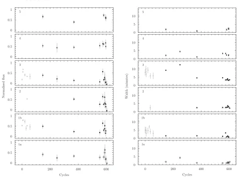
Our evaluation of the depth and the width of the dips
are presented in Figure 7. The measurement was done for
the 2014 data (except dips 1c). We calculated the flux at the
position/phase measured in Figure6. The width is measured
at the level where the normalised flux is equal to 1. In the
case of connecting dips, such as dips1a–1band dips 2−3, the
flux values between the dips are often lower than 1. For this situation, we mark the start (or the end) of one dip at the phase with the highest flux between the two dips.
The intensity plots show a similar feature where all of the dips are found to fluctuate on short time scale (days). This fluctuation can be seen clearly for dips 1b and 3 after cycle 550 in all of the dips. This short time scale variability is also seen in the plots of the width of the dips. These vari-ations are also seen in the intensity and width plots during
cycle 0−57. However, the small fluctuations are much harder
to detect with the longer integration time, and the width is also difficult to be measured accurately. Hence, we faded out the data points for the first few light curves in 2014 January
(cycle 0−57) as these points have larger uncertainties
There-Num
b
er
of
dips
Num
b
er
of
dips
2014 2015
1 2
1a 1b
1c 2
3
4 5
0 250 500
Cycles 1.1
1.2
P
osition
(phase)
2500 3000 3500
Cycles 1.1
1.2
P
osition
(phase)
0 2 4 6 8
[image:10.595.71.528.86.363.2]0 2 4 6 8
Figure 6.Top panels: The total number of dips seen in each light curve in 2014 (left) and 2015 (right). The grey dots on the left panel represent the number of dips in the light curves taken with integration times longer than 30 seconds. The grey crosses on the right panel mark the orbital cycles where the dips are absent in the light curve. Bottom panels: The position of each dip in orbital phase. The data with longer exposures taken between Jan7−15are faded out with grey error bars.
fore, we cannot tell whether there was any short time-scale variability during that period.
We note that potentially similar dips were observed
be-fore in QS Vir (O’Donoghue et al. 2003) in the optical, and
in V471 Tau (Jensen et al. 1986) in X-rays. However, this
is the first time that such dips are well resolved in time and monitored over about 1.5 years at several wavelengths. The dips in QS Vir were also detected spectroscopically by Parsons et al.(2011), altough the material was not optically thick. Therefore, the dips in QS Vir as reported by the au-thors were seen only in the lines and not in the continuum
light. In Figure8we show the expected location of the dips in
J1021+1744 as observed on 2014 April 1, where they seem to cluster near the L5 point. Only little force is needed to hold material at an equilibrium point, which might explain why we found the materials in J1021+1744 near the Lagrange L5 point. Opposite to the usual convention, the binary rotates clockwise in this figure.
It is interesting that in QS Vir and V471 Tau the dips are also reported to be in a very similar location close to
the L4/L5 “trojan” points.Jensen et al. (1986) found that
the X-ray dips in V471 Tau were seen near both L4 and L5 points, while the prominence material in QS Vir is located
close to its L5 point (Parsons et al. 2011).
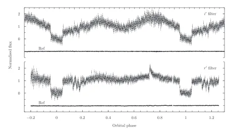
As a last remark, we report that we could, in a few cases, monitor J1021+1744 over a full orbit (see entries no 12, 18,
and 19 in Table 1). The data were taken in i′, r′, and g′,
consecutively. Two such light curves are presented in Figure
9. We, unfortunately, were unable to detect the dips’
mate-rial passing in front of the M dwarf. The secondary eclipse was also undetectable in any filter. We note however that on March 31 we observed a significant brightening, visible
around phase 0.72. The total intensity appeared to double and fade back within a few minutes. This is interpreted as a flare from the red dwarf, pointing to significant chromo-spheric activity. Whether such active behaviour is partly re-sponsible for mass ejections, which could funnel material to the observed dip positions, is an interesting possibility.
5 CONCLUSION
We have detected the signature of dips in the light curve of the detached, eclipsing white dwarf/M dwarf binary SDSS J1021+1744. Although potentially similar dips were seen before in a few other stars, such as in QS Vir (O’Donoghue et al. 2003) and in V471 Tau (Jensen et al.
1986), this is the first time that such dips are well resolved
in time and monitored over about 1.5 years in various filters across the whole visible spectrum. The dips are at locations which appear consistent with being close to the L5 point.
Our observations show that the dips are visible over hundreds of orbits, from a minimum of 3 months, possibly up
to 4−6 months and even up to 3 years. They also clearly
re-veal a complex dip structure, with their number, depth, and shape changing in time and as a function of wavelength. The
dip lifetimes are 3−100 times longer lived than prominences
on the Sun. On the other hand, the obscuration is probably also comparably larger, suggesting significant mass and den-sity of the blobs. It is noteworthy that the dips have depths
of as much as 30% of the total light in theu′ andg′ band,
showing that the material absorbs continuum and not just emission lines as in the case of the Sun.
Normalised
flux
1a 1b 2 3 4 5
0 200 400 600
Cycles 0
0.5 1 0 0.5 1 0 0.5 1 0 0.5 1 0 0.5 1 0 0.5 1
Width
(min
utes)
1a 1b 2 3 4 5
0 200 400 600
Cycles 0
[image:11.595.52.534.86.444.2]5 10 0 5 10 0 5 10 0 5 10 0 5 10 0 5 10
Figure 7.The plot of the flux (left) and the width (right) of the dips during the 2014 observation. The flux is rescaled to 0 during eclipse and 1 outside the eclipse (see text for details). In this manner, a value of 0 shows that there is more light being blocked by the dip. The out-of-eclipse part in ther′
filter is slightly higher due to the contribution from the secondary star, and the dips are shallower in the red filter. The width is measured at the top of the dips. The grey points (see 1b, 2 and 3) are for data with larger uncertainties (due to longer integration times and less resolution) obtained between January7−15.
form of blobs of gas or very extended prominences from the red dwarf star, is a new phenomenon to be reckoned with in models of PCEBs. Future monitoring of this binary, and other similar systems, is of crucial importance to understand the frequency of these occurrences and to learn more about their nature.
We have also provided a new ephemeris for the binary system, significantly improved over that of P13 thanks to a much longer time span. At the accuracy level of our data,
where the majority of the data in the O−C diagram are
scattered within±10 seconds from the zero value, we find
no evidence of changes in the primary mid-eclipse times.
ACKNOWLEDGMENTS
We thank the anonymous referee for valuable comments and suggestions which helped improved this paper. We also thank Boris Gaensicke for useful discussions. PI acknowl-edges the support from NRC-Thailand and a Royal Society International Exchange. TRM acknowledges the support of the Royal Society International Exchange Grant and of the Science and Technology Facilities Council under grant num-ber ST/L000733. NS and KC would like to thank Suranaree
University of Technology and the Office of Higher Education Commission for the partial support under the NRU project. SGP acknowledges financial support from FONDECYT in the form of grant number 3140585. This work has made use of data obtained at the Thai National Observatory on Doi Inthanon, operated by NARIT, and the WHT on La Palma.
REFERENCES
Abazajian K. N., et al., 2009,ApJS,182, 543
Briggs G. P., Ferrario L., Tout C. A., Wickramasinghe D. T., Hurley J. R., 2015,MNRAS,447, 1713
Copperwheat C. M., Marsh T. R., Dhillon V. S., Littlefair S. P., Hickman R., G¨ansicke B. T., Southworth J., 2010,MNRAS,
402, 1824
Dhillon V. S., et al., 2007,MNRAS,378, 825
Dhillon V. S., et al., 2014,MNRAS,444, 4009
Drake A. J., et al., 2009,ApJ,696, 870
Drake A. J., et al., 2014,MNRAS,441, 1186
Eastman J., Siverd R., Gaudi B. S., 2010,PASP,122, 935
Jensen K. A., Swank J. H., Petre R., Guinan E. F., Sion E. M., Shipman H. L., 1986,ApJ,309, L27
Figure 8. The Roche geometry of J1021+1744, scaled by the separation of the two stars. The dotted lines indicate the Roche lobe, while L1–L5 mark the positions of the Lagrangian points in this binary. The red dwarf star (solid black line) is seen very close to filling its Roche lobe. The straight lines indicate the line of sight to the white dwarf where the dips are seen on 2014 April 1. The binary rotates in clockwise direction.
O’Donoghue D., Koen C., Kilkenny D., Stobie R. S., Koester D., Bessell M. S., Hambly N., MacGillivray H., 2003,MNRAS,
345, 506
Parsons S. G., Marsh T. R., G¨ansicke B. T., Tappert C., 2011,
MNRAS,412, 2563
Parsons S. G., et al., 2013,MNRAS,429, 256
Parsons S. G., et al., 2015,MNRAS,449, 2194
Rebassa-Mansergas A., G¨ansicke B. T., Rodr´ıguez-Gil P., Schreiber M. R., Koester D., 2007,MNRAS,382, 1377
Rebassa-Mansergas A., Nebot G´omez-Mor´an A., Schreiber M. R., G¨ansicke B. T., Schwope A., Gallardo J., Koester D., 2012,
MNRAS,419, 806
Rebassa-Mansergas A., Agurto-Gangas C., Schreiber M. R., G¨ an-sicke B. T., Koester D., 2013,MNRAS,433, 3398
Webbink R. F., 1984,ApJ,277, 355
York D. G., et al., 2000,AJ,120, 1579
This paper has been typeset from a TEX/LATEX file prepared by
r′filter
i′filter
Ref Ref
Normalised
flux
−0.2 0 0.2 0.4 0.6 0.8 1 1.2
Orbital phase 0
[image:13.595.62.510.87.345.2]1 2 0 1 2
Figure 9.Full orbit light curves inr′
(2014 Mar 31) andi′
(2014 Jan 31) filters. The y-axis are scaled to 0 during the eclipse and 1 on the out-of-eclipse part (see text). The light curves of the reference star are marked as “Ref”. Ellipsoidal modulation is seen in both light curves, however this effect is more dominant in thei′ filter. Ther′-band light curve also exhibit a large flaring event at phase∼0.72.