Research Article
Open Access
S.J. Böing*
An object-based model for convective cold
pool dynamics
DOI 10.1515/mcwf-2016-0003
Received April 29, 2016; revised October 5, 2016; accepted November 15, 2016
Abstract:A simple model of the organization of atmospheric moist convection by cold outflows is presented. The model consists of two layers: a lower layer where instability gradually builds up, and an upper layer where instability is rapidly released. Its formulation is inspired by Abelian sandpile models: instability and convection are both represented in terms of particles that are coupled to a lattice grid. An excess of particles in the lower layer triggers a particle release into the upper (cloud) layer. Particles in the upper layer also induce particle movement in the lower layer: this reverse coupling represents the effect of precipitation and the associated cold outflows.
The model shows two behavioral regimes. Activity is scattered when the reverse coupling is weak, but when it is strong, convection forms cellular patterns. Though this model does not contain a detailed representation of physical processes in convection, it captures some key dynamical features of precipitating convection seen in satellite observations and LES studies. These include the formation of open cells, temporal oscillations in convective intensity, hysteresis, and the effect of precipitation on the scale of convection. We argue that an object-based representation of convection may be able to capture properties of convective organization that are missing in traditional parameterizations.
Keywords:cold pools, downdrafts, hysteresis, cellular automata, moist convection, cumulus, error growth
MSC:65C50 (numerical analysis: other computational problems in probability, 68Q80 (computer science: cellular automata), 86A10 (geophysics: meteorology and atmospheric physics), 37B15 (dynamical systems and ergodic theory: cellular automata)
1 Introduction
Satellite images of clouds show a wide variety of patterns, including scattered cumulus convection, open cells, closed cells and lines. These patterns are important in determining cloud cover, and hence the radia-tive budget of the atmosphere [e.g. 1]. One of the most prevalent patterns is open cellular convection. Figure 1a shows an example of the quasi-hexagonal cloud patterns which are typical for this type of convection. These patterns are observed both over land and over the ocean [2, 3], and often occur due to the influence of precipitation, both in cumulus [e.g. 4, 5] and stratocumulus [6] convection. Precipitation locally cools the subcloud layer air and suppresses convection, but as this cool air spreads out it leads to convergence of warm and moist air elsewhere.
The relative roles of forced lifting and moistening by surface fluxes in open cellular convection have been the topic of a number of previous studies [5, 7–10]. The availability of moist, unstable air is certainly important to create convection at the edge of regions that have been cooled by precipitation (so-called cold outflows or cold pools). However, the convection that occurs at the cold pool edges is mainly distinct from other cumulus clouds in the same domain because a) it is embedded in larger clouds and b) the larger role of dynamical
(a) (b)
Figure 1:a) Open cellular convection as seen from the International Space Station. Source: Wikimedia commons, public do-main. Courtesy NASA/JPL-Caltech. b) Pockets of open cells off the coast of Peru, as seen by Moderate Resolution Imaging Spec-troradiometer (MODIS) on NASA’s Aqua satellite. Source: Wikimedia commons, public domain. Courtesy: Jeff Schmaltz, NASA Earth Observatory.
lifting [5, 10], which is driven by convergence of boundary layer air into certain regions of the subcloud layer due to the spreading of cold pools.
Open cellular convection shows a wide range of interesting behaviors, including dependence on initial conditions. A previous study by Heus and Seifert [11] argues that both a regime with and a regime without cold pool organization can be found in cumulus simulations with the same large-scale forcings, but different initial conditions. In the case described in Heus and Seifert, the clouds which generate the precipitation have a horizontal dimension of a few hundred meters. These clouds are not explicitly resolved by current weather and regional climate models, and will likely remain underresolved by global climate models for decades to come. Heus and Seifert also show the differences in cumulus size statistics between the open cell and the unorganized regime: significantly larger clouds appear in the open cell regime.
In stratocumulus convection, pockets of open cells can sometimes also be embedded within areas of closed cell convection [1, 12, 13]. In this case, both the open and the closed cells show a degree of organization. Figure 1b shows an example of such a pocket of open cells. These pockets may indicate transitions from an open cell to a closed cell regime and vice versa. A recent study by Feingold et al. [14] discusses the reversibility of transitions between open and closed cell convection. In this study, it was found that the transition to open cell convection occurs much more rapidly than the reverse transition. Wang et al. [15] and Yamaguchi and Feingold [16] argue that the spacing between precipitation generating convective clouds is a key factor in determining whether or not a transition to open cell convection takes place. They refer to this as a ‘remote control’ mechanism.
two-dimensional model, where the presence of initially randomly distributed convection influences subse-quent time development through a distance-dependent stabilization/destabilization function. Feingold and Koren [22] described pattern formation in stratocumulus in terms of spatially coupled oscillators. Building on earlier work by Palmer [23], Shutts [24] used a lattice based (cellular automaton) approach to model convective variability by perturbing the vorticity field on the grid scale. Bengtsson et al. [25, 26] used cellular automata to introduce subgrid-scale variability, and the latter article introduces a representation of (cold pool) life time to represent the effects of outflows on convection. Cellular automaton models have the advantage that they can be trained using data from observations or cloud-resolving models, see e.g. Dorrestijn et al. [27].
Here, we will be exploring a different approach, which includes a description of the behavior of individ-ual convective cells as objects with an associated location and life time. Such an object-based approach has previously been used to develop parameterizations of deep and shallow cumulus convection by e.g. Plant and Craig and Sakradzija et al. [28–30]. In these previous studies, the cloud population was drawn from a distri-bution, rather than determined dynamically, and there was no horizontal communication except through the mean state.
The current work is distinct from previous approaches in that it prognostically determines a cloud size dis-tribution in a precipitating regime, and can therefore serve as a simple model for the formation of open cells. Although the model only has a limited set of rules that determine its dynamics (it can be coded efficiently in a few hundred lines), it is able to represent a number of phenomena that are present in cellular convection, such as quasi-hexagonal cell formation and different cloud sizes in precipitating and non-precipitating regimes. It is important to stress that this simple model is not a complete parameterization, but rather an exploration of the types of feedbacks that could be captured in an object-based parameterization. The model could be used as an ansatz for developing parameterizations, or as a crude way to introduce perturbations of which the length scale depends on rainfall in a weather or climate model. For models with mostly parameterized con-vection, current approaches include the cellular automaton approaches mentioned above and perturbation of physical tendencies [31, 32]: these approaches have been very successful, but it remains hard to represent different organizational modes of convection and long-range interactions. For convection-permitting models, introducing perturbations which depend on the boundary layer state is a path that is actively being explored [e.g. 33].
Other possible applications of our simple model include a testbed for convective-scale data-assimilation [c.f. 34, 35], or a simple representation of error-growth in precipitating and non-precipitating regimes [36, 37]. In future work, some of the processes could be replaced by representations that are closer to the actual physics of moist convection. In particular, the behavior of clouds could be described by models akin to those used for thermals and plumes in the fluid dynamics literature, and the subcloud layer could include a physical model of cold pool propagation (e.g. a shallow water model). Here, we are mainly interested in presenting a minimal model and showing it captures some key dynamical properties.
A python version of this model, using the scipy, matplotlib and pyqtgraph libraries, is freely available on gitlab (https://gitlab.com/sboeing/opencell, this version also contains some more recent work on linear organization in sheared convection).
2 Model description
2.1 Convective life cycle
The model consists of a lower layer (indicated with subscriptlow, subcloud) and an upper layer (subscript upp, cloud/rain). Both layers contain particles, which represent air that is becoming unstable with respect to moist convection (lower layer) or undergoing moist convection (upper layer). In order to determine when convection is released, the particles are coupled to a doubly-periodic grid of square cells with dimensionsNx
andNyin both layers. The cell edges are defined to have non-dimensional length 1. Particle velocities (to be
Particles are initiated in the lower layer. This represents the effects of radiative cooling and surface fluxes in gradually increasing moist convective instability. We do this by randomly drawing two real numbers from a uniform distribution,xp∼U([0,Nx]) andyp∼U([0,Ny]), that indicate where a particle is initially placed.
The number of particles to be seeded in each time step is drawn from a Poisson distribution with mean
rseedNxNy, whererseed is the average number of particles drawn per grid box per time step. Besides the
random location of particle initiation, the model is deterministic. If the instability in a lower layer grid cell becomes too large, i.e. if the cell contains a number of particles larger than some critical thresholdnc,
parti-cles are moved to the upper layer. In atmospheric terms, this corresponds to convective initiation, either by dynamical effects or because the level of free convection has been reached.
For the purely non-precipitating regime, we use an approach similar to an Abelian sandpile model in-troduced by Bak et al. [38, hereafter BTW], which is an existing model for representing phenomena with self-organized criticality. Such phenomena, which include earthquakes and certain types of avalanches, are characterized by a distribution of event magnitude which is a power-law over a certain range [e.g. 39]. It has been found in a number of studies that atmospheric convection also exhibits certain characteristics of self-organized criticality [e.g 40–42, the last of these studies also shows thermodynamic control in a way similar to homeostasis may be important], and it has been suggested that a sandpile model or alternatively a so-called Bak-Sneppen model [43] could be used as an analogue for convection. The current work is inspired by sandpile models, but also includes the effects of organization of convection by cold pools on the cloud size distribution. Though small cumulus cloud sizes and convective cluster sizes may follow such power-law scal-ing [11, 44–46], distributions of updraft mass-fluxes in cumulus convection seem to correspond better to an exponential or (mixed) Weibull distribution [29, 47, 48]. The model that develops here differs from the BTW sandpile model in some ways, and gives the latter type of distributions for cloud sizes in a regime with no organization (this may be because of the different way active cells can trigger their neighbors, see below).
We hypothesize a distribution of cloud size arises because cloud formation induces a positive feedback in the subcloud layer: in particular, the rising air leads to a low pressure below cloud base (Bernoulli suc-tion), which leads to convergence around the area where the cloud appears and stimulates further ascent [e.g. 49]. In the BTW sandpile model, the coupling between cells is realized by moving unstable particles to neighboring grid cells (for that model,nc= 4):
ifn(x,y) ≥ 4: (1)
n(x,y)→n(x,y) − 4
n(x± 1,y)→n(x± 1,y) + 1
n(x,y± 1)→n(x,y± 1) + 1
In our case, the domain is periodic and we would like to remove instability by moving particles to the upper layer, rather than to neighboring cells. At the same time, we want to keep a coupling which induces con-vection in neighboring cells. We achieve this by introducing a variableslowwhich indicates if neighbors are
undergoing convection, and lowering the threshold for instability to a lower valuennif this is the case. A
difference to the BTW sandpile model is that a cell cannot ‘receive’ additional instability when two or more of the cells around it, rather than one, become unstable.
slow(:, :) = 0 (2)
ifnlow(x,y) ≥nc:
nupp(x,y)→nlow(x,y)
nlow(x,y)→0
slow(x± 1,y)→1
if(nlow(x,y) ≥nn)and(slow(x,y) = 1):
nupp(x,y)→nlow(x,y)
nlow(x,y)→0
slow(x± 1,y)→1
slow(x,y± 1)→1
We refer to the transport of particles from the lower to the upper layer in a set of connected (4-connected, i.e. involvingx± 1,yorx,y± 1) cells as a trigger event. Multiple such trigger events may take place in the domain during a single time step. During the simulation, we keep track of the number of particles associated with each trigger eventMt, and the area (number of grid cells) associated with trigger eventsAt.
The particles are moved to the upper layer and classified as non-precipitating during a timetdelay. The
presence of a non-precipitating phase allows larger clouds to develop without immediately introducing a negative feedback due to cold pool formation. Subsequently, particles are relabeled as rain, and removed after a number of time stepstdur. In the current work, the life time of particles in the upper layer is a constant
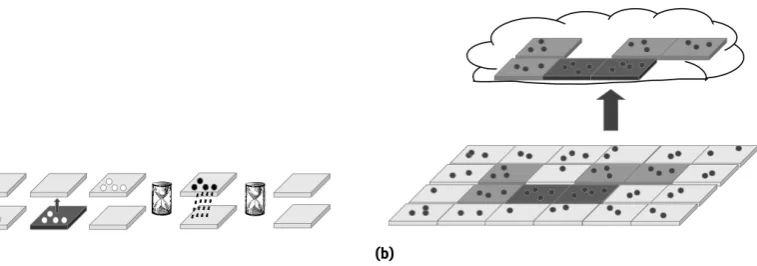
[image:5.595.84.463.335.468.2]number of time steps, though it may be physically more realistic to couple life time to cloud size [29]. The life cycle of particles and the mechanism by which particles are moved to the upper layer are illustrated in Figure 2.
(a) (b)
Figure 2:a) Schematic of the life cycle of particles in the model. b) Illustration of the way in which trigger events are diagnosed using thresholds for instability (the darkest cells) and for instability triggered by neighbors (one shade lighter).
2.2 Rain clusters
Once significant precipitation is initiated, a feedback between the cloud layer and the subcloud layer leads to organization into cellular patterns. We represent this feedback as the divergence of boundary layer instability away from regions where precipitation occurs.
A rain cluster is a 4-connected set of grid points in the upper layer that have rain particles in them (this definition is refined below). In order to determine these clusters, rain particles in the upper layer are counted on the grid as well: the number of rain particles in each cell is denoted asnrain. Each cluster has a magnitude
M, which is the number of particles in it, an areaAand perimeterp(the number of cell edges at the border
of the cluster). Each cluster is also associated with a center of mass of particle locations. In determining this center of mass, we use a mean of circular quantities to take into account the periodic boundary conditions.
p. Starting from a seed cell (which are evaluated in the order in which upper layer particles appeared on the grid), clusters are grown using a flood fill algorithm (this is also known as a paint-bucket fill, in this algorithm clusters of 4-connected points are determined). A buffer is kept with the cells added during the previous iteration, which initially contains the seed cell. During each iteration the cells neighboring those in the buffer are added, provided these new cells hold precipitating particles. At the start of each iteration, an additional criterionp< 4c√A, withca scaling parameter is checked in order to continue (c = 1 would
correspond to square cells, we usec= 5). This prevents elongated structures from appearing as a single rain cluster.
2.3 Precipitation feedbacks
The key feedback that needs to be captured is that the presence of precipitation locally suppresses convection in the sub-cloud layer, but leads to convergence and enhanced precipitation elsewhere. This is achieved by adding a velocity to the lower layer particles which moves them away from the precipitating convection. As a consequence, the release of instability is forced to occur over a small part of the domain. The velocity with which the particles move away from a rain cloud is given by a function f which operates on the vector~r
between the rain cluster center of mass and the particle and the magnitude of the rain clusterM.
~v=f(~r,M) (3)
From an implementation perspective, the crucial propertyfhas to have is that it is isotropic. The following implementation is used in the results we discuss:
if(M>m): (4)
~v= α √
M−m |~r|+d
~r |~r|
Here,αis a scaling constant,mis the minimum size of a rain cloud anddserves to limit the maximum
ve-locity. The appearance of a square root in the numerator is inspired by scaling laws for gravity currents, but the formulation could be refined using theoretical results [50–52]. For simplicity and computational efficiency, only the rain cluster that corresponds to the smallest value of the weighted distancew= (|~r|+d)/√M−macts on each particle, taking into account the periodicity of the domain (wmonotonically increases with distance).
This approach has been inspired by earlier work in computer-aided architecture [53].
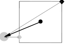
[image:6.595.117.533.522.638.2](a) (b)
Figure 3:Illustration of the mechanisms by which a) convergence of air due to clouds acts on the lower layer, which leads to b) triggering of new convective cells.
and there is some sensitivity to time step length. This can be noticed in e.g. the width of lines where particles converge, which is narrower for smaller time steps. In order to obtain narrow convergence lines, without increasing the computational cost by too much, we integrate particle movement with time steps which are smaller than those used in the main procedure and have decreasing length (0.4, 0.3, 0.2 and 0.1∆t, where∆t
is the full time-step length). For each of these time substeps and for each of the particles, we solve for its final position by integrating equation 4 over the substep. For the simplified case of a particle atx> 0 moving away
from a cloud atx= 0 in one dimension, the solution after a timeδtis:
x(t0+δt) =
q
2α√M−mδt+ (x(t0) +d)2−d (5) Due to this approach, a small value fordcan be chosen without introducing large numerical errors. This
completes the description of the model. An overview of the parameters and the values we used for these in our default setup is given in table 1.
2.4 Implementation
In the most straightforward implementation, where the velocity generated by each rain cluster is evaluated for each particle, the computational cost of the algorithm scales as the product of the number of particles in the lower layer and the number of rain clustersnlow,domainNclusters. This makes the computation expensive on large grids. In order to speed up computation, ‘candidate rain clusters’ are first computed on an inter-mediate grid, in the computations here this interinter-mediate grid has dimensions 64 × 64, whereas simulations are executed on a 640×640 domain. The computational cost is now determined by two factors, first the cost of calculating the candidate clusters on the intermediate grid, which scales with the number of cells on the intermediate grid and the number of rain clusters, and then second the cost of the step in which the rele-vant cluster is selected from these candidates. This second step scales as the number of candidate clusters per intermediate grid cell and the number of particles. For the first 1000 time steps of the ‘Low_Threshold’ simulation (see below), for example, the speedup is a factor 20 (the faster version ran in 255 seconds here).
For each intermediate grid cell, we first determine an upper bound onwfor each rain clusterc,wub,c. In
order to do this, we consider a maximum distance within the intermediate grid cell for each rain cluster. Here, we use the distance to the grid center and add half a grid cell length in each direction. The minimum of each of these upper bounds is an upper bound onwfor all particles in the intermediate grid cell, and is referred to aswub(the minimum is used since we consider the smallest weighted distance). Subsequently we determine
a lower bound for each intermediate grid cell and each clusterwlb,cby considering a minimum distance to the rain cluster within the grid cell, and only retain rain clusters for whichwlb,c < wub. Currently, a single
[image:7.595.206.338.561.651.2]intermediate grid is implemented, but in principle a number of grids with increasing level of refinement could be used to improve efficiency on large domains.
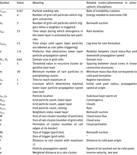
Table 1:Overview of model parameters and variable names, default values, and related atmospheric phenomena/scales.
Symbol Value Meaning Related scales/phenomena in
atmo-spheric simulations
rseed 0.03 Particle seeding rate Rate of instability creation
nc 4 Number of grid cell particles which
trig-gers convection
Energy needed to overcome CIN
nn 3 Number of grid cell particles which
trig-gers when a neighbor is triggered
Bernoulli suction
tdur 25 Time steps during which divergence in
the lower layer is activated by rain parti-cles
Rain duration
tdelay 15 Time steps until upper layer particles are labeled as rain (after triggering)
Lag time for rain formation
α 1.0 Prefactor that determines lower layer
particle propagation speed
Relation between cloud mass-flux and downdraft propagation speed
Nx,Ny 640 Domain size in grid cells Domain size
c 5 Threshold value in recursive cluster
al-gorithm (see text)
Spacing between cloud cores in linear convective structures
m 30 Minimum number of rain particles in
precipitating cluster
Minimum mass-flux that corresponds to cold pool formation
tm 1 Time to reach maximumm Regime transitions
d 1 Constant which determines maximal
lower layer particle propagation speed (see text)
Initial cold pool radius, propagation speed at origin
xp,yp Particle location Subcloud layer warm air
nlow Grid particle count, lower layer Convergence
nupp Grid particle count, upper layer Clouds
nrain Grid particle count, raining Rain
slow Neighbors state, lower layer Bernoulli suction
M Size of rain cluster (number of particles) Cloud mass-flux
A Size of rain cluster (number of grid cells) Cloud area
p Perimeter of cluster (number of cell
edges at its border)
Cloud perimeter
Mt Size of trigger (particles) Bernoulli suction
At Size of trigger (grid cells) "
~r Distance to rain cluster with maximum
|~v|
Distance to cold pool origin
~v Particle propagation speed Speed of air pushed out by cold pools
w Weighted distance to a rain cluster Inverse velocity, see text
3 Model behavior
3.1 Size distributions, hexagonal cell formation, scale growth
Figure 5 shows the distribution of the size of trigger events (both in terms ofAtandMt) in two simulations
convec-Table 2:Overview of model settings in different simulations
Simulation name nc nn mend tm Perturb*
Trigger_4_3 4 3 ∞ 1 No
Trigger_6_3 6 3 ∞ 1 No
No_Threshold 4 3 0 1 No
Low_Threshold 4 3 30 1 No
High_Threshold 4 3 48 1 No
Hysteresis 4 3 48 200 No
POCS 4 3 46 1 No
Pert_growth 4 3 30 1 Yes
* A single rain cluster is displaced by 0.01 cell length in the 1000th time step
(a) (b)
[image:9.595.49.501.87.211.2](c) (d)
Figure 5:Statistics of the area and magnitude of trigger events in the ‘Trigger_4_3’ (top) and ‘Trigger_6_3’ (bottom) simula-tions, in which precipitation feedbacks are absent. Note different scales are used for thex-axis.
tion without neighbors (nc = 4 andnc = 6, respectively). Table 1 and table 2 provide more details on the
simulations, these results correspond to the ‘Trigger_4_3’ and ‘Trigger_6_3’ simulations.
The distributions ofAtappear approximately exponential in both cases, but show some fluctuations at
higher values as the distribution becomes undersampled. There are additional fluctuations inMt, but these
can also be explained. Whennc = 4 andnn = 3, for example, trigger events with a particle countnc+knn,
withk∈Z≥0occur relatively frequently. Other values occur only because multiple particles are added to the
grid during each iteration.
[image:9.595.57.466.238.557.2]ncandnnare integer numbers, but this constraint could be removed in principle, for example by giving each
of the particles a weight drawn from a probability distribution.
[image:10.595.116.519.114.339.2](a) (b)
Figure 6:Example of model behavior in the ‘No_Threshold’ simulation a) lower-level particles and rain clusters b) gridded upper-level rain particle counts (shading) and rain clusters after 1000 time steps. Only part of the domain is shown. Rain clus-ters are shown as circles with size proportional toM. See Figure 7 for color shading.
We now consider the precipitating model. The case where the minimum rain cluster size m = 0 (‘No_Threshold’ simulation in table 2) is discussed first. Figure 6 shows the particle locations in the lower layer and the rain clusters after 1000 time steps in part of the domain. The rain clusters are numerous but remain relatively small (in terms of the associated number of grid cells) and the quasi-hexagonal cells that form in both the upper and the lower layer tend to be small as well.
In the remainder, simulations with a higher choice of the minimum cluster sizemwill be considered. This
seems the relevant case for understanding atmospheric cold pools, as very small clouds do not create cold pools on the ground. A choice of highermmakes rain clusters occur less frequently, and enables the field to
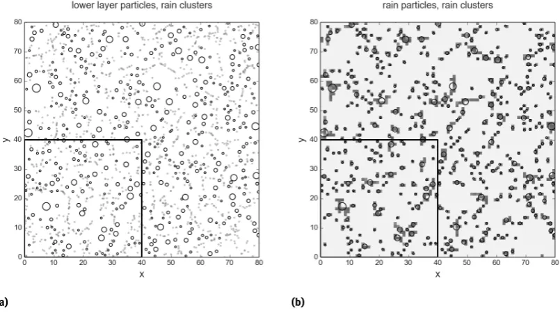
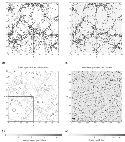
organize. As there are fewer rain clusters,~rneeds to be evaluated fewer times, which increases computation speed. Figure 7 shows the location of particles as well as rain clusters for the choicem= 30 (‘Low_Threshold’
case) after 1000 time steps. The clusters are much bigger in this simulation than in the ‘No_Threshold’ simula-tion. In Figure 7a, both precipitating and non-precipitating particles in the upper layer are shown. This Figure shows the location of non-precipitating particles is shifted with respect to the precipitating ones: the location of the rain clusters evolves over time. Figure 7b shows the detected rain clusters, which now widely vary in scale. In the lower layer, particle numbers are very low in the vicinity of precipitation clusters (Figure 7c) and the pattern of open cells is largely similar over the entire domain (Figure 7d).
Figure 8 shows the growth of the scale of these cells during the initial phase of the simulation. Cells start out small, but after some time an equilibrium scale is developed. This scale is determined by the speed at which particles propagate away from rain clusters.
3.2 Overshoots, meso-scale fluctutations and lags
(a) (b)
[image:11.595.52.472.77.552.2](c) (d)
Figure 7:Example of model behavior in the ‘Low_Threshold’ simulation (see text/table 2) a) upper-level particles and rain clus-ters b) upper-level particle counts and rain clusclus-ters and c) lower-level particles counts and rain clusclus-ters d) lower-level particle counts and rain clusters after 1000 time steps. Panels a-c show only part of the domain. The square window indicates the sub-domain on which further statistics are calculated (see text). Only rain clusters withM>mare shown.
(a) (b)
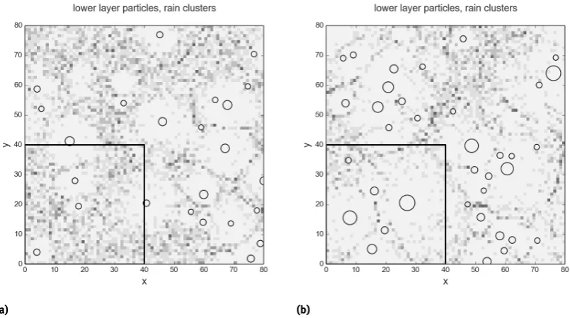
Figure 8:Scale growth in the ‘Low_Threshold’ simulation: lower-level particle counts and rain clusters after a) 100 and b) 400 time steps.
layer dries and cools [see, e.g. Figure 4 in reference 8] and convection is able to sustain itself with a subcloud layer that is on average colder and drier.
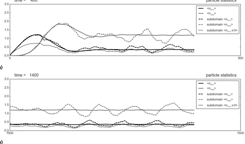
Figure 9b shows the same statistics, but during a later phase of the simulation. The subdomain statistics now show relatively large temporal fluctuations, similar to those observed in time-series of rain rate in the presence of cold pools [54]. The particle number in the upper layer clearly follows the particle number in the lower layer with a lag, which indicates particles that enter the subdomain tend to be locally removed from the lower layer.
3.3 Hysteresis, pockets of cells
If a high value ofmis used, there may be too few and too weak rain clusters to force a transition to open cell
behavior. An example of the model behavior in a simulation with a high value ofm(48) is shown in figure
10a. Although rain events occur, they rarely lead to the onset of convergence zones. However, if the threshold
mis introduced gradually during the initial 200 time steps, an irreversible transition to open cell behavior
takes place. Figure 10b shows the lower layer particle counts and rain clusters after 1000 time steps in a simu-lation where the value ofmis linearly increased from 0 to 48 over the first 200 time steps. Open cell behavior
reinforces itself once it has been initiated, and can persist under conditions where it would otherwise not be initiated. The open cell regime corresponds to much bigger rain clusters (figure 11). In both case the tails of the distributions look exponential, but for the lower values in the organized regime a power law distribution may be more appropriate (as demonstrated by the the log-log plots in figure 11). In the precipitating case, the number of small clouds is higher than expected from an exponential distribution, which may indicate the distribution is composed of two modes, as in the study by Sakradzija et al. [29].
When a value ofmis chosen that is close to the critical value that distinguishes presence or absence of
open cells, initiation may be relatively rare and large parts of the domain may transition to open cell behavior starting from a single point in the domain. This leads to the formation of a pocket of open cells. Figure 10c shows an example of this behavior (herem=46). This simulation eventually returned to a state without open
cells, which suggests the behavior may be transient. A simulation with slightly lowerm, however, continues
(a)
[image:13.595.56.476.71.317.2](b)
Figure 9:Normalized particle counts in the upper and lower layer, and fraction of cells with particles in them in the lower layer during a) the first phase and b) between 1000-1400 time steps in the ‘Low_Threshold’ simulation.
part of the parameter space sampled in our sensitivity experiments. They may, however, also appear in case the underlying model parameters were to vary slowly in space and time.
3.4 Perturbation growth
As a last example, we show a result from a simulation where one of the rain clusters in the upper layer appears displaced by 0.01 cell length during a single time step. This perturbation is introduced in the calculation of lower layer velocities, otherwise the simulation is identical to the ‘Low_Threshold’ simulation (note that this requires the random number generation to be reproducable). This experiment demonstrates the use of the model as a convective scale laboratory, which could be used to learn about error growth and test convective scale data assimilation techniques. Figure 12a shows the difference in lower layer gridded particle counts between this perturbed simulation and the ‘Low_Threshold’ simulation 100 time steps after the perturbation is introduced. The perturbed simulation develops in a different way, with cells initiating in slightly different positions, which gives rise to the double cell patterns visible in figure 12a. The perturbation is initially local but subsequently spreads over the domain, and also the difference in position of the cells between the simulations gradually increases. At a later stage, the cells are no longer simply shifted, but a truly different evolution has occurred (figure 12b).
4 Conclusions
(a) (b)
[image:14.595.113.513.69.529.2](c)
Figure 10:Lower layer gridded particle countsnlowand rain clusters (circles, size proportional toM) in a) the ‘High_Threshold’
simulation after 1000 time steps b) the ‘Hysteresis’ simulation after 1000 time steps c) the ‘POCS’ simulation after 400 time steps. See text for details.
including scale growth, open cell formation, hysteresis and pockets of open cells. The analogues are not exact, but the model shows that an object-based approach may be a good pathway towards including organi-zation in convective parameteriorgani-zations. The fact that all these behaviors occur suggests that these result from the long-range interactions in the system, which confirms the earlier ‘remote control’ hypothesis of Wang et al. [15] and Yamaguchi and Feingold [16]. It also suggests these behaviors may be found in a wide range of regimes.
(a) (b)
[image:15.595.58.466.68.385.2](c) (d)
Figure 11:Statistics of rain magnitudeMin the a) ‘High_Threshold’ and b) ‘Hysteresis’ simulations after 1000 time steps. c,d) idem, but on a log-log plot. Note different scales are used for thex-axis.
(a) (b)
[image:15.595.75.451.437.663.2]have to be taken that the cloud size statistics that result from the new framework are not too different from those resulting from previous approaches. The framework presented here lends itself to incorporating more accurate physical models of updrafts in particular. Bringing in a more physically-based model of downdrafts that describes both downdraft dynamics and thermodynamics may be more difficult. Recent studies on the bulk behavior of downdrafts [52] or shallow water models could serve as guidance here. Formulating approx-imate conservation laws for an object-based framework, as well as the interaction between updraft properties and the near-environment profiles of temperature, moisture and wind will also be key to further development of object-based parameterizations [48].
Acknowledgement: Colleagues at TU Delft and participants of the 2013 COST Cold Pool workshop in Bergen provided feedback which was useful for the development of this model. Richard Keane, Oliver Halliday and two anonymous reviewers provided constructive feedback on the draft. This work was funded through the Leeds-Met Office Academic Partnership.
References
[1] B. Stevens, G. Vali, K. Comstock, R. Wood, et al. Pockets of open cells and drizzle in marine stratocumulus. Bull. Am. Meteorol. Soc., 86(1):51, 2005.
[2] M. A. Lima and J. W. Wilson. Convective storm initiation in a moist tropical environment. Mon. Weath. Rev., 136(6):1847– 1864, 2008.
[3] J. H. Ruppert Jr and R. H. Johnson. Diurnally modulated cumulus moistening in the preonset stage of the Madden–Julian Oscillation during DYNAMO.J. Atmos. Sci, 72(4):1622–1647, 2015.
[4] M. Khairoutdinov and D. Randall. High-resolution simulation of shallow-to-deep convection transition over land.J. Atmos. Sci, 63(12):3421–3436, 2006.
[5] S. J. Böing, H. J. J. Jonker, A. P. Siebesma, and W. W. Grabowski. Influence of the subcloud layer on the development of a deep convective ensemble.J. Atmos. Sci, 69(9):2682–2697, 2012.
[6] H. Wang and G. Feingold. Modeling mesoscale cellular structures and drizzle in marine stratocumulus. Part I: impact of drizzle on the formation and evolution of open cells.J. Atmos. Sci, 66(11):3237–3256, 2009.
[7] A. M. Tompkins. Organization of tropical convection in low vertical wind shears: The role of cold pools.J. Atmos. Sci, 58(13): 1650–1672, 2001.
[8] L. Schlemmer and C. Hohenegger. The formation of wider and deeper clouds as a result of cold-pool dynamics. J. Atmos. Sci, 71(8):2842–2858, 2014.
[9] Z. Feng, S. Hagos, A. K. Rowe, C. D. Burleyson, M. N. Martini, and S. P. Szoeke. Mechanisms of convective cloud organization by cold pools over tropical warm ocean during the AMIE/DYNAMO field campaign. J. Adv. Mod. Earth. Sys., 7(2):357–381, 2015.
[10] N. Jeevanjee and D. M. Romps. Effective buoyancy, inertial pressure, and the mechanical generation of boundary layer mass flux by cold pools.J. Atmos. Sci, 72(8):3199–3213, 2015.
[11] T. Heus and A. Seifert. Automated tracking of shallow cumulus clouds in large domain, long duration Large Eddy Simulations.
Geosci. Model Dev. Disc., 6(2):2287–2323, 2013.
[12] C. S. Bretherton, T. Uttal, C. W. Fairall, S. E. Yuter, et al. The EPIC 2001 stratocumulus study.Bull. Am. Meteorol. Soc., 85(7): 967, 2004.
[13] A. Berner, C. Bretherton, and R. Wood. Large-eddy simulation of mesoscale dynamics and entrainment around a pocket of open cells observed in VOCALS-REx RF06.Atmos. Chem. Phys., 11(20):10525–10540, 2011.
[14] G. Feingold, I. Koren, T. Yamaguchi, and J. Kazil. On the reversibility of transitions between closed and open cellular con-vection.Atmos. Chem. Phys., 15(13):7351–7367, 2015.
[15] H. Wang, G. Feingold, R. Wood, and J. Kazil. Modelling microphysical and meteorological controls on precipitation and cloud cellular structures in Southeast Pacific stratocumulus.Atmos. Chem. Phys., 10(13):6347–6362, 2010.
[16] T. Yamaguchi and G. Feingold. On the relationship between open cellular convective cloud patterns and the spatial distri-bution of precipitation.Atmos. Chem. Phys., 15:1237–1251, 2015.
[17] B. Mapes and R. Neale. Parameterizing convective organization to escape the entrainment dilemma. J. Adv. Mod. Earth. Sys., 3:M06004, 2011.
[18] J.-Y. Grandpeix and J.-P. Lafore. A density current parameterization coupled with Emanuel’s convection scheme. Part I: the models.J. Atmos. Sci, 67:881–897, 2010.
[20] B. Khouider, J. Biello, A. J. Majda, et al. A stochastic multicloud model for tropical convection.Comm. in Math. Sciences, 8 (1):187–216, 2010.
[21] D. A. Randall and G. J. Huffman. A stochastic model of cumulus clumping.J. Atmos. Sci, 37(9):2068–2078, 1980.
[22] G. Feingold and I. Koren. A model of coupled oscillators applied to the aerosol–cloud–precipitation system.Nonlinear Proc. in Geophysics, 20(6):1011–1021, 2013.
[23] T. N. Palmer. A nonlinear dynamical perspective on model error: a proposal for non-local stochastic-dynamic parametrization in weather and climate prediction models.Quart. J. Roy. Meteorol. Soc., 127(572):279–304, 2001.
[24] G. Shutts. A kinetic energy backscatter algorithm for use in ensemble prediction systems.Quart. J. Roy. Meteorol. Soc., 131 (612):3079–3102, 2005.
[25] L. Bengtsson, H. Körnich, E. Källén, and G. Svensson. Large-scale dynamical response to subgrid-scale organization pro-vided by cellular automata.J. Atmos. Sci, 68(12):3132–3144, 2011.
[26] L. Bengtsson, M. Steinheimer, P. Bechtold, and J.-F. Geleyn. A stochastic parametrization for deep convection using cellular automata.Quart. J. Roy. Meteorol. Soc., 139(675):1533–1543, 2013.
[27] J. Dorrestijn, D. Crommelin, J. Biello, and S. Böing. A data-driven multi-cloud model for stochastic parametrization of deep convection.Phil. Trans. of the Roy. Soc. A, 371(1991), 2013.
[28] R. Plant and G. C. Craig. A stochastic parameterization for deep convection based on equilibrium statistics.J. Atmos. Sci, 65(1):87–105, 2008.
[29] M. Sakradzija, A. Seifert, and T. Heus. Fluctuations in a quasi-stationary shallow cumulus cloud ensemble.Nonlin. Processes Geophys., 1:1223–1282, 2014.
[30] G. C. Craig and B. G. Cohen. Fluctuations in an equilibrium convective ensemble. Part I: theoretical formulation.J. Atmos. Sci, 63(8):1996–2004, 2006.
[31] T. Palmer, R. Buizza, F. Doblas-Reyes, T. Jung, M. Leutbecher, G. Shutts, M. Steinheimer, and A. Weisheimer. Stochastic parametrization and model uncertainty. European Centre for Medium-Range Weather Forecasts, 2009.
[32] H. Christensen, I. Moroz, and T. Palmer. Stochastic and perturbed parameter representations of model uncertainty in con-vection parameterization.J. Atmos. Sci, 72(6):2525–2544, 2015.
[33] K. Kober and G. C. Craig. Physically-based stochastic perturbations (PSP) in the boundary layer to represent uncertainty in convective initiation.Journal of the Atmospheric Sciences, 2016.
[34] J. Harlim and A. Majda. Filtering nonlinear dynamical systems with linear stochastic models.Nonlinearity, 21(6):1281, 2008. [35] M. Würsch and G. C. Craig. A simple dynamical model of cumulus convection for data assimilation research.Met. Zeitschrift,
23(5):483–490, 2014.
[36] C. Hohenegger and C. Schär. Predictability and error growth dynamics in cloud-resolving models. J. Atmos. Sci, 64(12): 4467–4478, 2007.
[37] T. Selz and G. C. Craig. Upscale error growth in a high-resolution simulation of a summertime weather event over Europe.
Mon. Weath. Rev., 143(3):813–827, 2015.
[38] P. Bak, C. Tang, K. Wiesenfeld, et al. Self-organized criticality: an explanation of 1/f noise.Phys. Rev. Lett., 59(4):381–384, 1987.
[39] R. Dickman, M. A. Muñoz, A. Vespignani, and S. Zapperi. Paths to self-organized criticality.Braz. J. of Phys., 30(1):27–41, 2000.
[40] O. Peters, C. Hertlein, and K. Christensen. A complexity view of rainfall.Phys. Rev. Lett., 88(1):018701, 2001. [41] O. Peters and J. D. Neelin. Critical phenomena in atmospheric precipitation.Nature physics, 2(6):393–396, 2006. [42] J.-I. Yano, C. Liu, and M. W. Moncrieff. Self-organized criticality and homeostasis in atmospheric convective organization.
Journal of the Atmospheric Sciences, 69(12):3449–3462, 2012.
[43] F. Spineanu, M. Vlad, and D. Palade. Regimes of self-organized criticality in the atmospheric convection. "arXiv, 1404.4538, 2014.
[44] R. Neggers, H. Jonker, and A. Siebesma. Size statistics of cumulus cloud populations in large-eddy simulations.J. Atmos. Sci, 60(8):1060–1074, 2003.
[45] O. Peters, J. D. Neelin, and S. W. Nesbitt. Mesoscale convective systems and critical clusters.J. Atmos. Sci, 66(9):2913–2924, 2009.
[46] R. Wood and P. R. Field. The distribution of cloud horizontal sizes.J. Clim., 24(18):4800–4816, 2011.
[47] B. G. Cohen and G. C. Craig. Fluctuations in an equilibrium convective ensemble. Part II: numerical experiments.J. Atmos. Sci, 63(8):2005–2015, 2006.
[48] R. Keane and R. Plant. Large-scale length and time-scales for use with stochastic convective parametrization.Quart. J. Roy. Meteorol. Soc., 138(666):1150–1164, 2012.
[49] B. E. Mapes. Gregarious tropical convection.Journal of the atmospheric sciences, 50(13):2026–2037, 1993.
[50] A. Ross, A. Tompkins, and D. Parker. Simple models of the role of surface fluxes in convective cold pool evolution.J. Atmos. Sci, 61(13):1582–1595, 2004.
[51] F. Pantillon, P. Knippertz, J. H. Marsham, and C. E. Birch. A parameterization of convective dust storms for models with mass-flux convection schemes.J. Atmos. Sci, 72(6):2545–2561, 2015.
[53] P. Coates. Review paper: some experiments using agent modelling at CECA. InProc. .7th Generative Art Conf. (GA2004), pages 14–16. Generative Design Lab, 2004.
[54] G. Feingold, I. Koren, H. Wang, H. Xue, and W. A. Brewer. Precipitation-generated oscillations in open cellular cloud fields.
Nature, 466(7308):849–852, 2010.
[55] R. Neggers. Exploring bin-macrophysics models for moist convective transport and clouds.Journal of Advances in Modeling Earth Systems, 7(4):2079–2104, 2015.